Second International Nurse Rostering Competition (INRC-II)
— Problem Description and Rules —

Abstract

In this paper, we provide all information to participate to the Second International Nurse Rostering Competition (INRC-II). First, we describe the problem formulation, which, differently from INRC-I, is a multi-stage procedure. Second, we illustrate all the necessary infrastructure do be used together with the participant’s solver, including the testbed, the file formats, and the validation/simulation tools. Finally, we state the rules of the competition. All update-to-date information about the competition is available at http://mobiz.vives.be/inrc2/.

1 Introduction

Nurse rostering is a very important problem in healthcare management. Early papers date from the seventies, but especially in the last decade, it has drawn significant attention; see [4, 5] for a review of literature and a classification.

The First International Nurse Rostering Competition (INRC-I) [8] was run in 2010. The competition welcomed 15 submissions in three categories (sprint, medium and long tracks). Since then, several research groups took this formulation and the corresponding instances as a challenge [1, 3, 6, 7, 11, 9, 12] and produced remarkable results. Optimal solutions as well as new best solutions have also been found and reported.

The problem considered for INRC-I was the assignment of nurses to shifts in a fixed planning horizon, subject to a large number of hard and soft constraint types.

For the Second International Nurse Rostering Competition (INRC-II), we propose a smaller set of constraint types, but within a multi-stage formulation of the problem. That is, the solvers of the participants are requested to deal with a sequence of cases, referring to consecutive weeks of a longer planning horizon (4 or 8 weeks).

The search method designed by the participants has to be able to solve a single stage of the problem corresponding to one week. Some information, called history, is carried out between consecutive weeks, so that the one coming from the previous week has to be taken into account by the solver. The history includes border data, such as the last worked shift of each nurse, and counters for cumulative data, such as total worked night shifts. Counters’ value has to be checked against global thresholds, but only at the end of the planning period. The planning horizon is not rolling [2] but fixed, in the sense that in the final week all counters are checked against their limits.

We provide a simple command-line simulation/validation software to be used simulate the solution process and to evaluate the quality of the solver. The simulator invokes the participant’s solver for each stage iteratively, then updates the history after each single execution. The provided validator concatenates the solutions for all weeks, and evaluates them all together, along with the cumulative data coming from the final history.

The solver should take into account the following separate input sources:

Scenario:

Information that is global to all weeks of the entire planning horizon, such as nurse contracts and shift types.

Week data:

Specific data of the single week, like daily coverage requirements and nurse preferences for specific days.

History:

Information that must be passed from a week to the other, in order to compute constraint violations properly. It includes border information and global counters.

The solver must deliver an output file, based on which, the simulator computes the new history file, to be passed back to the solver for the solution of the next week. As will be explained further, besides the mandatory input and output files, a custom data file may be used to exchange information between two stages.

The paper is organised as follows. Section 2 illustrates the problem definition. Section 3 describes the testbed. Section 4 shows the software tools made available to the participants to evaluate their solver. Finally, Section 5 describes the rules of the competition. Appendix A describes the file formats and Appendix B provides a deeper look at the constraint evaluation. All update-to-date information about the competition is available at http://mobiz.vives.be/inrc2/.

2 Problem definition

The basic (one-stage) problem consists in the weekly scheduling of a fixed number of nurses using a set of shifts, such that in each day a nurse works a shift or has a day-off. Nurses may have multiple skills, and for each skill we are given different coverage requirements.

Given the multi-stage nature of the overall process, the input data of the problem comes from three different sources, called scenario, week data, and history, as explained in the following sections. The way the information is organised in the files is explained in Appendix A.

2.1 Scenario

The scenario represents the general data common to all stages of the overall process. It contains the following information:

Planning horizon:

The number of weeks that compose the planning period.

Skills:

The list of skills included in the problem (head nurse, regular nurse, trainee, …). Each nurse has one or more skills, but in each working shift she/he covers exactly one skill request.

Contracts:

Each nurse has one specific contract (full time, part time, on call, …). The contract sets limits on the distribution and the number of assignments within the planning horizon. In detail, it contains:

• minimum and maximum total number of assignments in the planning horizon;

• minimum and maximum number of consecutive working days;

• minimum and maximum number of consecutive days-off;

• maximum number of working week-ends in the planning horizon;

• a Boolean value representing the presence of the Complete week-end constraint to the nurse, which states that the nurse should work both days of the week-end or none of them.

Nurses:

For each nurse, the name (identifier), the contract and the set of skills are given.

Shift types:

For each shift type (early, late, night, …), it is given the minimum and maximum number of consecutive assignments of that specific type, and a matrix of forbidden shift type successions is given. For example, it may not be allowed to assign to a nurse an early shift the day after a late one.

2.2 Week data

The week data contains the specific data for the single week. It consists of the following information:

Requirements:

It is given, for each shift, for each skill, for each week day, the optimal and minimum number of nurses necessary to fulfil the working duties.

Nurse requests:

It is given, a set of triples, each one composed by the nurse name, the week day, and a shift. The presence of a given triple represents the request of the nurse not to work in the given shift in the given day. The special shift name Any represents the request of not working in any shift of the day, i.e. having a day-off.

The above information varies from week to week, due to variability on the number of current patients and specific preferences of nurses.

Conventionally, all weeks start with Monday, so that the data is stored in the order Mon, Tue, …, Sun.

2.3 History

The history contains the information that must be carried over from one week to the following one, so as to evaluate the constraints correctly. In detail, it reports for each nurse the following two types of information:

Border data:

The border data is used for checking the constraints on consecutive assignments. They are:

• shift worked in the last day of the previous week, or the special value None if the nurse had a day-off;

• number of consecutive worked shifts of the same type and number of consecutive worked shifts in general (both are 0 if the last worked shift is None);

• number of consecutive days-off (0 if the last worked shift is not None).

Counters:

The counters collect the cumulative value over the weeks of specific quantities of interest, that have to be checked only at the end of the planning period. They are:

• total number of worked shifts;

• total number of worked week-ends.

The history is computed after each week based on the solution delivered by the solver and on the previous history. The history passed to the solver for the first week has all counter values equal to 0, whereas the border data can have any value.

2.4 Solution

The full solution process is a loop that executes at each step the solver for a week, iterating for all weeks in the planning period (4 or 8 weeks).

After each week, the history information is computed based on the solution and the previous history, and delivered in a new file. This is done by the simulator provided, whereas the solver must deliver only the solution itself.

The complete process is sketched in Figure 1(a), assuming a scenario of 4 weeks. Input files are colored in different shades of cyan, and the output ones in different shades on magenta.

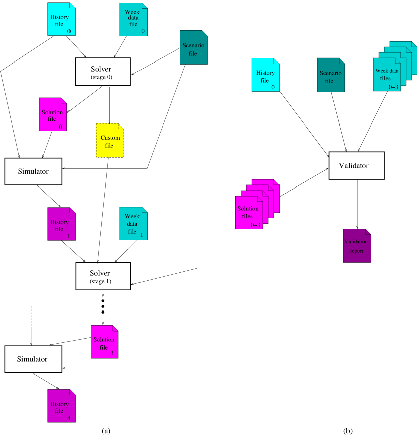
Figure 1: The overall solution/simulation/validation process (4 weeks).

In addition to generating a solution file after solving each stage, the solver might want to save some other prediction information in a custom file (in yellow in Figure 1) and passing it to the next solver call, in order to guide the solving of the next stage better. The content and the format of this file is free, but its name is set by the simulator, as described in Section 4.1.

The output produced by the solver is a list of assignments of nurses to shifts and skills. Each entry contains the nurse name, the week day, the shift, and the skill. As an example, consider the entry $\langle$Mary, Tue, Night, HeadNurse$\rangle$, that states that the nurse Mary works on Tuesday the night shift with the role of head nurse.

The quality of the overall solution is evaluated, as shown in Figure 1(b), for the entire planning horizon based on:

• the solution for each week containing the assignments of the nurses to shifts and skills, using the requirements in the week data file and the border data in the history file;

• the counters of the final history file, against the limits provided in the scenario.

2.5 Constraints

According to the setting outlined above, we split the constraints into two sets: those that can be computed for each week separately, and those that are computed only globally at the end of the planning period.

As customary, they are also split into hard and soft constraints. The former must be always satisfied, and the latter contribute to the objective function. The weight of each single soft constraint is shown prior to its description below.

2.5.1 Constraints on the single week

Below is the list of hard (H) and soft (S) constraint types:

H1. Single assignment per day:

A nurse can be assigned to at most one shift per day.

H2. Under-staffing:

The number of nurses for each shift for each skill must be at least equal to the minimum requirement.

H3. Shift type successions:

The shift type assignments of one nurse in two consecutive days must belong to the legal successions provided in the scenario.

H4. Missing required skill:

A shift of a given skill must necessarily be fulfilled by a nurse having that skill.

S1. Insufficient staffing for optimal coverage (30):

The number of nurses for each shift for each skill must be equal to the optimal requirement. Each missing nurse is penalised according to the weight provided. Extra nurses above the optimal value are not considered in the cost.

S2. Consecutive assignments (15/30):

Minimum and maximum number of consecutive assignments, per shift or global, should be respected. Their evaluation involves also the border data. Each extra or missing day is multiplied by the corresponding weight. The weights for consecutive shift constraint and for consecutive working days are respectively 15 and 30.

S3. Consecutive days off (30):

Minimum and maximum number of consecutive days off should be respected. Their evaluation involves also the border data. Each extra or missing day is multiplied by the corresponding weight.

S4. Preferences (10):

Each assignment to an undesired shift is penalised by the corresponding weight.

S5. Complete week-end (30):

Every nurse that has the complete weekend value set to $true$, must work both week-end days or none. If she/he works only one of the two days Sat and Sun this is penalised by the corresponding weight.

2.5.2 Constraints spanning over the planning horizon

The following (soft) constraints are evaluated only at the end of the planning period:

S6. Total assignments (20):

For each nurse the total number of assignments (working days) must be included within the limits (minimum and maximum) enforced by her/his contract. The difference (in either direction), multiplied by its weight, is added to the objective function.

S7. Total working week-ends (30):

For each nurse the number of working weed-ends must be less than or equal to the maximum. The number of worked week-ends in excess is added to the objective function multiplied by the weight. A week-end is considered “working” if at least one of the two days (Sat and Sun) is busy for the nurse.

Obviously, the solver should take constraints S6 and S7 into account in each single stage. However, their violation values have a decreasing degree of uncertainty going from one week to the following one, and only in the last week they can be evaluated exactly. It is up to the solver to decide the way to model them in the cost function in the previous weeks.

3 Instances

One complete solution process requires as input a scenario, an initial history, and 4 (or 8) week data, and it produces 4 (or 8) week solutions and one final history. Scenario, week data, history, and week solutions are written in separate files each one with its own syntax.

For ease of processing, all files are provided in XML, JSON, and text-only formats, and each participant can use the format that he/she considers as most convenient for his/her implementation. File formats are explained in Appendix A.

Files belonging to the same case are grouped in a dataset, which is composed by the following set of files:

• 1 scenario file;

• 3 initial history files;

• 10 week data files.

An instance is thus a specific scenario, an initial history, and a sequence of 4 (or 8) week data files, all belonging to the same dataset. The same week data file can also be used multiple times in the same instance.

We provide a testbed composed of 14 datasets, one for each combination of number of weeks and number of nurses, taken from the sets {30,40,50,60,80,100,120} and {4,8}, respectively. Datasets are named using these two number with the prefixes n (for nurses) and w for weeks. For example, the dataset n050w8 is the (unique) one with 50 nurses and 8 weeks.

In addition, three test datasets, n005w4, n012w8, and n012w4, are provided for testing and debugging purposes. For the test datasets, we also provide the solution for three specific instances.

The instances of the competition testbed that will be used for evaluating the participants will be released on May 15^th as the late data.

4 Tools

We provide to the participants a suite of software tools. The simulator manages the multi-stage solution process. The validator certificates the quality of a given instance. The benchmark executable computes the allowed running time for each computer. Finally, the feasibility checker gives the possibility to the participant to check that a specific instance of a given dataset has or not at least one solution that satisfies all hard constraints.

4.1 Simulator

On the competition website, the java program Simulator.jar that runs the simulation and delivers the costs is available. As shown in Figure 1, the simulator receives a scenario file, an initial history file, the solver’s executable file name and a sequence of week data files as its input. It then applies the solver on each week data file, generating a history file for each stage based on the solution obtained from each solver call. After the last week data file in the sequence is solved, the validator is called to evaluate the whole planning horizon. Besides the basic input described above, the user can also specify random seeds for his/her solver, the directory where the solver is run in, and the directory where all solution files, generated history files, log files (the solver’s console output after each solver call) and the validator’s results are saved in. In addition to generating a solution file after solving each stage, the solver might want to save some other information in a custom file and passing it to the next solver call, in order to guide the solving of the next stage better. Such a need is also supported by the simulator.

The simulator is called using the following command line parameters (parameters in the square brackets are optional):

java -jar Simulator.jar --sce <Scenario_File> --his <Initial_History_File>
--weeks <Week_Data_File_1> .. <Week_Data_File_N> --solver <Solver_Executable>
[--runDir <Running_Directory>] [--outDir <Output_Directory>] [--cus]
[--rand <Random_Seed_1> .. <Random_Seed_N>]

In detail:

• File names of the scenario file, initial history files, and week data files can have either absolute or relative path. If they are relative, they will be taken from the current working directory (not the Running_Directory).

• The number of week data files N must be equal to the number of weeks stated in the scenario file.

• Before each solver’s call, the command line cd <Running_Directory> will be called.

• The number of random seeds specified after the --rand option can be either one or N. If only one random seed is given, it will be used for all solver’s calls.

The simulator works under the assumption that the solver has the following command line:

Solver_Executable --sce <Scenario_File> --his <Initial_History_File>
--week <Week_Data_File> --sol <Solution_File_Name>
[--cusIn <Custom_Input_File>] [--cusOut <Custom_Output_File>] [--rand <Random_Seed>]

The simulator generates the following files in the directory Output_Directory:

• history-week0.<extension>, history-week1.<extension>, ..., history-weekN.<extension>: history files generated by the simulator after each solver call. The <extension> is set based on the relevant input file format.

• custom-week0, custom-week1, ..., custom-weekN: custom files generated by the solver, if the --cus option is used.

• result-week0.txt, result-week1.txt, ..., result-weekN.txt: log files for all solver calls.

• Validator-results.txt: results of the validator.

The simulator asks the solver to generate a single solution file for each stage. These solution files are also located in the directory Output_Directory, under the names sol-week0.<extension>, sol-week1.<extension>, ..., sol-weekN.<extension>.

Important note: the simulator and the validator must be in the same directory.

As an example, the command line for the simulator

java -jar Simulator.jar --his H0-n005w4-0.txt --sce Sc-n005w4.txt
--weeks WD-n005w4-2.txt WD-n005w4-0.txt WD-n005w4-2.txt WD-n005w4-1.txt
--solver ./program.exe --runDir Devel/ --outDir Simulator_out/
--cus --rand 10 11 12 13

produces the following subsequent command lines

cd Devel/

./program.exe --sce /home/nguyen/data/Sc-n005w4.txt --his /home/nguyen/data/H0-n005w4-0.txt
--week /home/nguyen/data/WD-n005w4-2.txt --sol /home/nguyen/data/Simulator_out/sol-week0.txt
--cusOut /home/nguyen/data/Simulator_out/custom-week0 --rand 10

./program.exe --sce /home/nguyen/data/Sc-n005w4.txt
--his /home/nguyen/data/Simulator_out/history-week0.txt
--week /home/nguyen/data/WD-n005w4-0.txt --sol /home/nguyen/data/Simulator_out/sol-week1.txt
--cusIn /home/nguyen/data/Simulator_out/custom-week0
--cusOut /home/nguyen/data/Simulator_out/custom-week1 --rand 11

./program.exe --sce /home/nguyen/data/Sc-n005w4.txt
--his /home/nguyen/data/Simulator_out/history-week1.txt
--week /home/nguyen/data/WD-n005w4-2.txt --sol /home/nguyen/data/Simulator_out/sol-week2.txt
--cusIn /home/nguyen/data/Simulator_out/custom-week1
--cusOut /home/nguyen/data/Simulator_out/custom-week2 --rand 12

./program.exe --sce /home/nguyen/data/Sc-n005w4.txt
--his /home/nguyen/data/Simulator_out/history-week2.txt
--week /home/nguyen/data/WD-n005w4-1.txt --sol /home/nguyen/data/Simulator_out/sol-week3.txt
--cusIn /home/nguyen/data/Simulator_out/custom-week2
--cusOut /home/nguyen/data/Simulator_out/custom-week3 --rand 13

Given that the current working directory is /home/nguyen/data/

4.2 Validator

The validator is a java program that checks for the validity of a solution of an instance, and calculate the corresponding objective function value according to the evaluation method (see also Appendix B) and the constraints’ weights described in Section 2.4. The validator is automatically called by the simulator at the end of the solving procedure. It can also be used as a stand-alone program with the following syntax:

java -jar Validator.jar --sce <Scenario_File> --his <Initial_History_File>
--weeks <Week_Data_File_1> .. <Week_Data_File_N>
--sols <Solution_File_1> .. <Solution_File_N> [--verbose]

If the --verbose option is used, details of each soft constraint’s violation of each nurse are shown. As an example, the command line

java -jar validator.jar --sce n005w4/Sc-n005w4.txt --his n005w4/H0-n005w4-0.txt
--weeks n005w4/WD-n005w4-1.txt n005w4/WD-n005w4-2.txt n005w4/WD-n005w4-3.txt
n005w4/WD-n005w4-3.txt --sols Solutions/Sol-n005w4-1-0.txt Solutions/Sol-n005w4-2-1.txt
Solutions/Sol-n005w4-3-2.txt Solutions/Sol-n005w4-3-3.txt

produces an output like:

        |M|T|W|T|F|S|S| |M|T|W|T|F|S|S| |M|T|W|T|F|S|S| |M|T|W|T|F|S|S|
-------------------------------------------------------------------------
Patrick |N|-|E|E|E|L|L| |-|-|E|E|L|L|L| |-|N|N|N|N|N|N| |-|L|L|L|L|N|N|
Andrea  |L|L|-|-|L|L|L| |N|N|N|N|N|-|L| |L|L|L|-|-|N|N| |N|N|N|-|-|E|E|
Stefaan |N|N|N|N|-|-|-| |E|E|L|L|-|-|E| |N|N|-|-|E|E|E| |N|N|-|-|-|L|L|
Sara    |-|-|-|N|N|N|N| |N|-|-|-|E|E|E| |E|L|L|L|-|-|-| |E|E|E|E|E|-|-|
Nguyen  |E|E|L|L|-|E|E| |L|L|-|L|N|N|N| |-|E|E|E|L|L|L| |-|L|L|N|N|N|N|

Hard constraint violations
--------------------------
Minimal coverage constraints: 0
Required skill constraints: 0
Illegal shift type succession constraints: 0
Single assignment per day: 0

Cost per constraint type
------------------------
Total assignment constraints: 320
Consecutive constraints: 465
Non working days constraints: 330
Preferences: 70
Max working weekend: 210
Complete weekends: 60
Optimal coverage constraints: 240

------------------------
Total cost: 1695

4.3 Benchmark

The benchmark program is designed to test how fast your machine is at doing the sort of things that are involved in rostering. For each problem size, which is defined as the number of nurses in the scenario file, the program tells you how long you can run your algorithm for each stage. It is not possible to provide perfectly equitable benchmarks across many platforms and algorithms, and we know that the benchmark may be kinder to some people than others. It is pointed out that all the finalists will be run on a standard machine therefore creating a ‘level playing field’.

The benchmark is only suitable for individual, single processor machines. It is not suitable, for example, for specialist parallel machines or clusters. In general, for multi-core machines, one single core is allowed to be used for the competition.

The benchmark is provided as an executable for various architectures. If your architecture is not among the ones provided please contact us to obtain the program.

The program should be run when the machine is not being used for anything else. The program will report how long it took, and hence the length of time you can run your rostering algorithm per stage, for each number of nurses.

On a relatively modern PC, the benchmark program will grant the participant approximately $10+30*(N-20)$ seconds for each stage, in which $N$ is the number nurses.

4.4 Feasibility Checker

It could be possible that some instance created from a given dataset is infeasible. In order to prevent participants from wasting time for searching for feasible solutions when they do not exists, a feasibility checker is provided. This tool is a web service and can be found on the competition website from November 5, 2014.

5 Competition rules

5.1 General rules

This competition seeks to encourage research into automated nurse rostering methods for solving a multi-stage nurse rostering problem, and to offer prizes to the most successful methods. It is the spirit of these rules that is important, not the letter. With any set of rules for any competition it is possible to work within the letter of the rules but outside the spirit.

Rule 1:

The organisers reserve the right to disqualify any participant from the competition at any time if the participant is determined by the organisers to have worked outside the spirit of the competition rules. The organisers’ decision is final in any matter.

Rule 2:

The organisers reserve the right to change the rules at any time, if they believe it is necessary for the sake of preserving the correct operation of the competition. Any change of rules will be accompanied by a general email to all participants.

Rule 3:

The competition has a deadline when all submissions must be uploaded. The deadline is strict and no extensions will be given under any circumstances.

Rule 4:

Participants can use any programming language. The use of third-party software is allowed under the following restrictions:

• it is free software;

• it’s behaviour is (reasonably) documented;

• it runs under a commonly-used operating system (Unix/Linux, Windows, or Mac OS X).

Rule 5:

Participants have to benchmark their machine with the program provided in order to know how much time they have available to run their program for each stage on their machines. The solver should run on a single core of the machine.

Rule 6:

The solver should take as input the files in one of the formats described, and produce as output a list of solution files for all stages (in the same format). It should do so within the allowed CPU time.

Rule 7:

The solver used should be the same executable for all weeks, but obviously internally it could exploit the information regarding the week it is solving, and adapt its behavior depending on it.

Rule 8:

The solver can be either deterministic or stochastic. In both cases, participants must be prepared to show that the results are repeatable in the given computer time. In particular, the participants that use a stochastic algorithm should code their program in such a way that the exact run that produced each solution submitted can be repeated (by recording the random seed).

Rule 9:

Along with the solution for each instance, the participants should also submit a concise and clear description of their algorithm, so that in principle others can implement it.

Rule 10:

A set of 5 finalists will be chosen after the competition deadline. Ordering of participants will be based on the scores obtained on the provided instances. The actual list will be based on the ranks of solvers on each single instance. The mean average of the ranks will produce the final place list. More details on how the orderings will be established can be found in Section 5.3.

Rule 11:

The finalists will be asked to provide the executable that will be run and tested by the organisers. The finalists’ solvers will be rerun by the organisers on new instances (including new datasets). It is the responsibility of the participant to ensure all information is provided to enable the organisers to recreate the solution. If appropriate information is not received or indeed the submitted solutions cannot be recreated, another finalist will be chosen from the original participants.

Rule 12:

Finalists’ eventual place listings will be based on the ranks on each single instance for a set of trials on all instances. As with Rule 10, an explanation of the procedures to be used can be found in Section 5.3.

Rule 13:

In some circumstances, finalists may be required to show source code to the organisers. This is simply to check that they have stuck to the rules and will be treated in the strictest confidence.

Rule 14:

Organisers of the competition cannot participate to it.

5.2 Dates

The competition starts on October 17, 2014. On this date, we release the datasets, this specification paper, the simulator, the validator and the benchmark program. The web service for the feasibility checker is available on November 5, 2014. On May 15, 2015, the late data, i.e., a list of specific instances created from the competition testbed, will be released. The deadline for submission of participants’ best results and their solvers is June 1, 2015. Notifications of the finalists will be sent out on July 1, 2015. The winners will be announced at the MISTA 2015 Conference in Prague (August 25-27, 2015).

5.3 Adjudication procedure

We follow the same adjudication procedure of INRC-I [8], from which in turn has been imported from the Second International Timetabling Competition (ITC-2007) [10]. It is repeated here for the sake on selfcontainedness.

Let $m$ be the total number of instances and $k$ be the number of participants. Let $X_{ij}$ be the value of the objective function $s$ supplied (and verified) by participant $i$ for instance $j$. In case participant $i$ provides an infeasible solution for instance $j$ or he/she does not provide it at all, $X_{ij}$ is assigned a conventional value $M$ larger than all the results supplied by the other participants for that instance.

The matrix $X$ of results is transformed into a matrix of ranks $R$ assigning to each $R_{ij}$ a value from $1$ to $k$. That is, for instance $j$ the supplied $X_{1j}$, $X_{2j}$, …,$X_{kj}$ are compared with each other and the rank $1$ is assigned to the smallest observed value, the rank $2$ to the second smallest, and so on to the rank $k$, which is assigned to the largest value for instance $ij$. We use average ranks in case of ties.

Consider the example with $m=6$ instances and $k=7$ participants in Table 1. The ranks are shown in Table 2.

Instance	1	2	3	4	5	6
Solver 1	34	35	42	32	10	12
Solver 2	32	24	44	33	13	15
Solver 3	33	36	30	12	10	17
Solver 4	36	32	46	32	12	13
Solver 5	37	30	43	29	9	4
Solver 6	68	29	41	55	10	5
Solver 7	36	30	43	58	10	4

Table 1: An example of scores of the submitted solutions.

Instance	1	2	3	4	5	6
Solver 1	3	6	3	3.5	3.5	4
Solver 2	1	1	6	5	7	6
Solver 3	2	7	1	1	3.5	7
Solver 4	4.5	5	7	3.5	6	5
Solver 5	6	3.5	4.5	2	1	1.5
Solver 6	7	2	2	6	3.5	3
Solver 7	4.5	3.5	4.5	7	3.5	1.5

Table 2: Corresponding solution ranks for the example.

We define for each solver the mean of the ranks. The finalists of the competition will be the 5 solvers with the lowest mean ranks. In case of a tie for entering the last positions, all the last equal-mean solvers are included in the final (in this case the finalists will be more than 5). In the example, the mean ranks are shown in Table 3. In this case the finalists would be solvers 1, 3, 5, 6 and 7.

Solver 1	3.83
Solver 2	4.33
Solver 3	3.58
Solver 4	5.17
Solver 5	3.08
Solver 6	3.92
Solver 7	4.08

Table 3: Mean ranks.

The organisers will check the runs of the candidate finalist with the submitted seed to make sure that the submitted runs are repeatable. If they are not, then another entrant will be chosen for the final.

For the final, the same evaluation process is repeated for the finalists with the following differences:

1. New instances, including hidden datasets, will be used.

2. The solvers will be run by the organisers, thus the finalist should give support to the organisers in the process of compiling and running the solvers.

3. For each instance, the organisers will run 10 independent trails with seeds chosen at random. For each trial, we will compute the ranks and average them on all trials on all instances.

The winner is the one with the lowest mean rank. In case of a tie, 1 trial is added for all instances until a single winner is found.

5.4 Prizes

The top three will divide € 1729 among them (first prize € 819, second € 637, third € 273), and will be offered free registration to PATAT 2016, that will include a special track on the competition.

Appendix A File formats

In this appendix we describe the format for the input files (scenario, week data, and history) and output file (solution). Only the text-only format is explained in details, given that XML and JSON files are organised with the same structure, but in a more self-explanatory way.

Scenario

The first line of the scenario file contains the name of the dataset in the format nXXXwY, where XXX is the number of nurses and Y the number of weeks of the planning horizon. This is the identifier of the scenario that is subsequently used in the relating history, week data, and solution files.

SCENARIO = n005w4

Then it is reported the length of the planning horizon, expressed in number of weeks, and the number and names of skills for nurses.

WEEKS = 4

SKILLS = 2
HeadNurse
Nurse

The shift types section indicates the number of shift types available, and for each one, the identifier (its name), and the minimum and the maximum number of consecutive assignments allowed. For each shift type, it is also detailed the forbidden shift types sequences as $\langle$preceding_shift_type$\rangle$ $\langle$number_forbidden_successions$\rangle$ $\langle$succeeding_shift_type_list$\rangle$. In the following example, the successions Late $\rightarrow$ Early, Night $\rightarrow$ Early and Night $\rightarrow$ Late are forbidden.

SHIFT_TYPES = 3
Early (2,5)
Late (2,3)
Night (4,5)

FORBIDDEN_SHIFT_TYPES_SUCCESSIONS
Early 0
Late 1 Early
Night 2 Early Late

In the contract section it is listed the name of the contract type, and the lower and upper limits on working and rest days. In detail, it establishes the minimum and the maximum number of total assignments in the planning horizon, the minimum and the maximum number of consecutive working days, the minimum and the maximum number of consecutive days off, the maximum number of working weekends, and the presence (1) or absence (0) of the complete weekend constraint.

CONTRACTS = 2
FullTime (15,22) (3,5) (2,3) 2 1
PartTime (7,11) (3,5) (3,5) 2 1

Finally, the nurse section reports the total number of nurses available, and for each nurse his/her identifier (the name), the contract type, the number of skills owned and their names.

NURSES = 5
Patrick FullTime 2 HeadNurse Nurse
Andrea FullTime 2 HeadNurse Nurse
Stefaan PartTime 2 HeadNurse Nurse
Sara PartTime 1 Nurse
Nguyen FullTime 1 Nurse

Week data

In the week data file, first of all there is the identifier of the corresponding scenario; then all the data about coverage requirements and nurse preferences is listed.

WEEK_DATA
n005w4

A coverage requirement is specified by the shift type, the skill, and for each day of the week (from Monday to Sunday), the minimum coverage and the optimal coverage.

REQUIREMENTS
Early HeadNurse (1,1) (0,0) (0,0) (0,0) (0,0) (1,1) (0,0)
Early Nurse (1,2) (1,1) (1,1) (0,1) (1,1) (1,1) (0,1)
Late HeadNurse (1,1) (0,1) (1,1) (0,0) (0,0) (0,0) (0,0)
Late Nurse (1,1) (1,1) (0,1) (0,1) (1,1) (1,1) (1,1)
Night HeadNurse (0,0) (1,1) (0,0) (0,0) (1,1) (1,1) (0,0)
Night Nurse (0,1) (1,1) (1,1) (1,1) (1,1) (0,1) (1,1)

Finally, the number of shift off requests is reported with the following grammar: $\langle$nurse$\rangle$ $\langle$shift type$\rangle$ $\langle$day$\rangle$. The special shift type Any means that the nurse would like to have a day off.

SHIFT_OFF_REQUESTS = 3
Sara Any Thu
Sara Night Sat
Stefaan Late Sat

History

The first line of the history file describes the week to which the history refers to (i.e. $0$ for the initial history file, $1$ after the first week, …) and the relating scenario file.

HISTORY
0 n005w4

In addition, the file contains the nurse history, in terms of total number of assignments, total number of worked weekends, last assigned shift type, number of consecutive assignments of the last shift type, number of consecutive worked days and number of consecutive days off.

NURSE_HISTORY
Patrick 0 0 Night 1 4 0
Andrea 0 0 Early 3 3 0
Stefaan 0 0 None 0 0 3
Sara 0 0 Late 1 4 0
Nguyen 0 0 None 0 0 1

Solution

The solution file gives the assignment of nurses to shifts and skills. The file starts with the reference to the solved week and to the scenario.

SOLUTION
3 n005w4

Then each single assignment is shown (in any order), reporting the name of the nurse, the day, the shift type and the skill considered. Days off are neglected.

ASSIGNMENTS = 26
Patrick Mon Late HeadNurse
Patrick Tue Night HeadNurse
Patrick Fri Early Nurse
Patrick Sat Early Nurse
Patrick Sun Late Nurse
Andrea Mon Early HeadNurse
Andrea Tue Late Nurse
..
Nguyen Fri Late Nurse
Nguyen Sat Late Nurse
Nguyen Sun Night Nurse

Appendix B Constraint evaluation

In this appendix, we explain in more detail some of the constraints presented in Section 2.5. Specifically, we believe that the constraints that involve border data (history file) need a deeper explanation. Conversely, constraints H1, H2, S1, S4, S5, S6, and S7 do not rely on border data for their evaluation, and, in our opinion, their evaluation is straightforward and not subject to ambiguous interpretation.

For the remaining constraints, we exhaustively describe their evaluation at both borders of a stage.

In the descriptions that follow, for simplicity, we omit the weight of the (soft) constraints, and we focus on the amount of the violation. For simplicity, we assume that the input data is the one included in the following fragment of a scenario file, setting all limits to the same value 3.

SHIFT_TYPES = 2
Early (3,3)
Late (3,3)

FORBIDDEN_SHIFT_TYPES_SUCCESSIONS
Early 0
Late 1 Early

CONTRACTS = 1
FullTime (...,...) (3,3) (3,3) ...

Section B.1 explains the number of consecutive working days constraints (S2). In section B.2 the evaluation of the number of consecutive days off constraints is explained (S3). Section B.3 elaborates on the forbidden shift type successions constraint (H3).

B.1 Number of consecutive assignments (S2)

Maximum number of consecutive working days

The evaluation of the constraint at the start of a stage depends on the value $c$ of the number of consecutive working days at the beginning of a stage (from history). In Table 4, the constraint is evaluated for $c=5$, showing for clarity also the week before the planning period.

The symbol $\bullet$ is used to mean any working shift, and the symbol – means a day off. An empty cell is used for assignments irrelevant for the example under consideration.

As it can be seen, the evaluator only counts the ‘extra’ amount of violation, as part of the violation has already been taken into account during the evaluation of the previous stage (see table 6).

Previous period

Current period

Mo

Tu

We

Th

Fr

Sa

Su

Mo

Tu

We

Th

Fr

Sa

Su

Violations

–

$\bullet$

$\bullet$

$\bullet$

$\bullet$

$\bullet$

–

0

–

$\bullet$

$\bullet$

$\bullet$

$\bullet$

$\bullet$

$\bullet$

–

1

–

$\bullet$

$\bullet$

$\bullet$

$\bullet$

$\bullet$

$\bullet$

$\bullet$

–

2

Table 4: Evaluation of the maximum number of consecutive working days constraint at the beginning of a stage.

From this point on, the previous planning period will be represented by a single column denoting the value of the relevant counter from history. Table 5 shows the evaluation of the constraint for different values of $c$.

History	Mo	Tu	We	Th	Fr	Sa	Su	Violations
$c\geq 3$	–							0
	$\bullet$	–						1
	$\bullet$	$\bullet$	–					2
	$\bullet$	$\bullet$	$\bullet$	–				3
	$\bullet$	$\bullet$	$\bullet$	$\bullet$	–			4
$c=2$	–							0
	$\bullet$	–						0
	$\bullet$	$\bullet$	–					1
	$\bullet$	$\bullet$	$\bullet$	–				2
	$\bullet$	$\bullet$	$\bullet$	$\bullet$	–			3
$c=1$	–							0
	$\bullet$	–						0
	$\bullet$	$\bullet$	–					0
	$\bullet$	$\bullet$	$\bullet$	–				1
	$\bullet$	$\bullet$	$\bullet$	$\bullet$	–			2
$c=0$	–							0
	$\bullet$	–						0
	$\bullet$	$\bullet$	–					0
	$\bullet$	$\bullet$	$\bullet$	–				0
	$\bullet$	$\bullet$	$\bullet$	$\bullet$	–			1

Table 5: Evaluation of the maximum number of consecutive working days constraint at the beginning of a stage for different values of $c$.

Table 6 shows the evaluation of the constraint for the maximum consecutive working days at the end of a stage.

Mo	Tu	We	Th	Fr	Sa	Su	Violations
–	$\bullet$	$\bullet$	$\bullet$	$\bullet$	$\bullet$	$\bullet$	3
	–	$\bullet$	$\bullet$	$\bullet$	$\bullet$	$\bullet$	2
		–	$\bullet$	$\bullet$	$\bullet$	$\bullet$	1
			–	$\bullet$	$\bullet$	$\bullet$	0

Table 6: Evaluation of the maximum number of consecutive working days constraint at the end of a stage.

Minimum number of consecutive working days

Table 7 evaluates the constraint for the minimum consecutive working days. If $c\geq 3$, then no violation of this constraint can occur at the beginning of a stage. As it is uncertain what the assignments at the beginning of the next stage are, the minimum number of consecutive working days constraint is not taken into account at the end of a stage.

History	Mo	Tu	We	Th	Fr	Sa	Su	Violations
c = 2	–							1
	$\bullet$	–						0
c = 1	–							2
	$\bullet$	–						1
	$\bullet$	$\bullet$	–					0
c = 0	–							0
	$\bullet$	–						2
	$\bullet$	$\bullet$	–					1
	$\bullet$	$\bullet$	$\bullet$	–				0

Table 7: Evaluation of the minimum number of consecutive working days constraint at the beginning of a stage.

Note that both the maximum and minimum constraints are evaluated per series. In Table 8, there are two series of length 1 and 2, respectively, that produce two and one violations, respectively (minimum is 3).

Mo	Tu	We	Th	Fr	Sa	Su	Violations
–	$\bullet$	–	–	$\bullet$	$\bullet$	–	3

Table 8: Evaluation of the minimum number of consecutive working days constraint for two series.

Minimum and maximum number of consecutive assignments to the same shift

The examples presented in the previous paragraphs work similarly for the consecutive assignments to the same shift, by replacing the symbol $\bullet$ with the specific shift (E or L, in this example) and the symbol – with a day off or any shift different from the given one.

B.2 Number of consecutive days off (S3)

B.2.1 Maximum number of consecutive days off

The evaluation of the constraint at the start of a stage depends on the value of the number of consecutive days off from the history, that we call $c$ again. Table 9 shows the evaluation of the maximum number of consecutive days off constraint at the beginning of the stage.

History	Mo	Tu	We	Th	Fr	Sa	Su	Violations
$c\geq 3$	$\bullet$							0
	–	$\bullet$						1
	–	–	$\bullet$					2
	–	–	–	$\bullet$				3
	–	–	–	–	$\bullet$			4
$c=2$	$\bullet$							0
	–	$\bullet$						0
	–	–	$\bullet$					1
	–	–	–	$\bullet$				2
	–	–	–	–	$\bullet$			3
$c=1$	$\bullet$							0
	–	$\bullet$						0
	–	–	$\bullet$					0
	–	–	–	$\bullet$				1
	–	–	–	–	$\bullet$			2
$c=0$	$\bullet$							0
	–	$\bullet$						0
	–	–	$\bullet$					0
	–	–	–	$\bullet$				0
	–	–	–	–	$\bullet$			1

Table 9: Evaluation of the maximum number of consecutive days off constraint at the beginning of a stage for different values of $c$.

In Table 10, we show the violations of the maximum number of consecutive days off constraint at the end of a stage; the history is not involve in this case.

Mo	Tu	We	Th	Fr	Sa	Su	Violations
			$\bullet$	–	–	–	0
		$\bullet$	–	–	–	–	1
	$\bullet$	–	–	–	–	–	2
$\bullet$	–	–	–	–	–	–	3

Table 10: Evaluation of the maximum number of consecutive days off constraint at the end of a stage.

B.2.2 Minimum number of consecutive days off

Table 11 shows the evaluation of the minimum number of consecutive days off constraint at the beginning of the stage.

History	Mo	Tu	We	Th	Fr	Sa	Su	Violations
$\geq 3$	$\bullet$							0
	–	$\bullet$						0
	–	–	$\bullet$					0
	–	–	–	$\bullet$				0
	–	–	–	–	$\bullet$			0
2	$\bullet$							1
	–	$\bullet$						0
	–	–	$\bullet$					0
	–	–	–	$\bullet$				0
	–	–	–	–	$\bullet$			0
1	$\bullet$							2
	–	$\bullet$						1
	–	–	$\bullet$					0
	–	–	–	$\bullet$				0
	–	–	–	–	$\bullet$			0
0	$\bullet$							0
	–	$\bullet$						2
	–	–	$\bullet$					1
	–	–	–	$\bullet$				0
	–	–	–	–	$\bullet$			0

Table 11: Evaluation of the minimum number of consecutive days off constraint at the beginning of a stage for different values of $c$.

B.3 Forbidden shift type successions

In Table 12, the evaluation of the constraint for the forbidden succession at the beginning of the stage is shown. As can be seen, the constraint is violated only when the last assigned shift type from history is equal to Late and the Monday shift is Early.

History	Mo	Tu	We	Th	Fr	Sa	Su	Violation
L	E							true
	L							false
	–							false
E	E							false
	L							false
	–							false

Table 12: Evaluation of the forbidden shift type succession L-E.

References

- [1] Mohammed A Awadallah, Ahamad Tajudin Khader, Mohammed Azmi Al-Betar, and Asaju La’aro Bolaji. Nurse rostering using modified harmony search algorithm. In Swarm, Evolutionary, and Memetic Computing, volume 7077 of Lecture Notes in Computer Science, pages 27–37. Springer, 2011.
- [2] Jonathan F Bard and Hadi W Purnomo. Short-term nurse scheduling in response to daily fluctuations in supply and demand. Health Care Management Science, 8(4):315–324, 2005.
- [3] Edmund K Burke and Tim Curtois. New approaches to nurse rostering benchmark instances. European Journal of Operational Research, 237(1):71–81, 2014.
- [4] Edmund K Burke, Patrick De Causmaecker, Greet Vanden Berghe, and Hendrik Van Landeghem. The state of the art of nurse rostering. Journal of Scheduling, 7(6):441–499, 2004.
- [5] Patrick De Causmaecker and Greet Vanden Berghe. A categorisation of nurse rostering problems. Journal of Scheduling, 14(1):3–16, 2011.
- [6] Federico Della Croce and Fabio Salassa. A variable neighborhood search based matheuristic for nurse rostering problems. Annals of Operations Research, 218(1):185–199, 2014.
- [7] Martin Josef Geiger. Personnel rostering by means of variable neighborhood search. In Operations Research Proceedings 2010, pages 219–224. Springer, 2011.
- [8] Stefaan Haspeslagh, Patrick De Causmaecker, Andrea Schaerf, and Martin Stølevik. The first international nurse rostering competition 2010. Annals of Operations Research, 218:221–236, 2014.
- [9] Zhipeng Lü and Jin-Kao Hao. Adaptive neighborhood search for nurse rostering. European Journal of Operational Research, 218(3):865–876, 2012.
- [10] Barry McCollum, Andrea Schaerf, Ben Paechter, Paul McMullan, Rhyd Lewis, Andrew J. Parkes, Luca Di Gaspero, Rong Qu, and Edmund K. Burke. Setting the research agenda in automated timetabling: The second international timetabling competition. INFORMS Journal on Computing, 22(1):120–130, 2010.
- [11] HG Santos, TAM Toffolo, S Ribas, and RAM Gomes. Integer programming techniques for the nurse rostering problem. Annals of Operations Research, pages 1–27, 2014. Online first.
- [12] Ioannis P Solos, Ioannis X Tassopoulos, and Grigorios N Beligiannis. A generic two-phase stochastic variable neighborhood approach for effectively solving the nurse rostering problem. Algorithms, 6(2):278–308, 2013.