Supplemental Material

We study two modifications to the Scrambler oscillator model analyzed in the main text. The first is the original model, but with alternative couplings between oscillators. Specifically, we change how close to threshold an oscillator has to be in order to be absorbed by a firing cluster. This only modestly changes the analysis.

The second is a more substantial alteration. When an oscillator reaches threshold, it no longer scrambles every other oscillator to a new, random, voltage. Instead, it kicks every other oscillator up by a constant amount, or up to threshold, whichever is less. This deterministic resetting rule is in line with the simplest traditional models of pulse-coupled oscillators. As will be shown, this change makes for a more involved analysis.

I Alternative Couplings

We first restate the dynamics of the original Scrambler model, and then describe the variations.

Recall that in the main text we considered a population of $N\gg 1$ integrate-and-fire oscillators coupled all-to-all. Each oscillator was characterized by a voltage-like state variable $x$, which increased linearly according to $\dot{x_{i}}=1$. When a cluster of $j$ oscillators reached a threshold value set to $1$, they fired and then instantly did three things: (i) they reassigned every other oscillator (or cluster of oscillators) a new voltage uniformly at random (they scrambled the oscillators) (ii) they absorbed any oscillators within a distance $j/N$ of threshold and (iii) they reset their voltage to 0 along with any oscillators they absorbed.

We now modify event (ii) in either of two ways: when a cluster of size $j$ fires, it either absorbs all oscillators within a new distance of threshold given by (a) $kj/N$ or (b) $k/N$. Modification (a) generalizes the original model by including an adjustable coupling $k$. Modification (b) assumes that the absorption region is independent of $j$, the size of the firing cluster.

These generalizations change the analysis of the Scrambler model only slightly. For instance, to find the disorder parameter $c(t)$, we again use the rate equation $\dot{c}=-\sum_{i}R_{i}L_{i}$, where $R_{i}$ denotes the rate at which a cluster of size $i$ fires, and $L_{i}$ denotes the number of oscillators absorbed when a cluster of size $i$ fires. In the original model, to find $L_{i}$ and $R_{i}$, we made liberal use of the fact that all oscillators on the interval $[1-j/N,1)$ were captured when a cluster of size $j$ fired. With the generalized couplings (absorption distances), this interval simply changes to $[1-kj/N,1)$ and $[1-k/N,1)$. This change propagates through the analysis straightforwardly. Hence, we state the results in the following table without derivation. (The special function $W(x)$ in the table refers to Lambert’s $W$ function.)

	$j/N$	$kj/N$	$k/N$
$L_{i}$	$ic$	$kic$	$kc$
$R_{i}$	$c_{i}/2$	$c_{i}/(1+k)$	$c_{i}/(1+kc)$
$c(t)$	$e^{-t/2}$	$e^{-\frac{k}{k+1}t}$	$1/(kW(k^{-1}e^{(k^{-1}+t)}))$

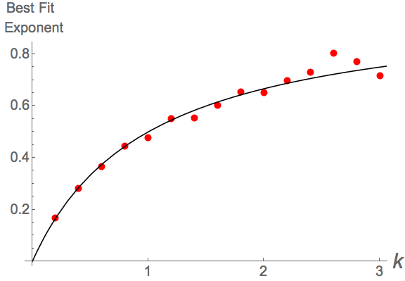
The rows of the table give the results for $L_{i},R_{i}$ and $c(t)$; the columns show how the results vary for the three coupling schemes: original, (a), and (b). For coupling scheme (a), where the absorption distance is $kj/N$, the exponential decay constant in $c(t)$ is predicted to be $-k/(k+1)$. To test this, we simulated $c(t)$ for various $k$, and found the exponents of best fit. Figure 1 shows the results along with the theoretical curve.

Figure 1: Magnitude of the decay constant in $c(t)$ for coupling scheme (a). Black curve, theoretical prediction $k/(k+1)$; red dots, simulation results for $N=5000$ oscillators.

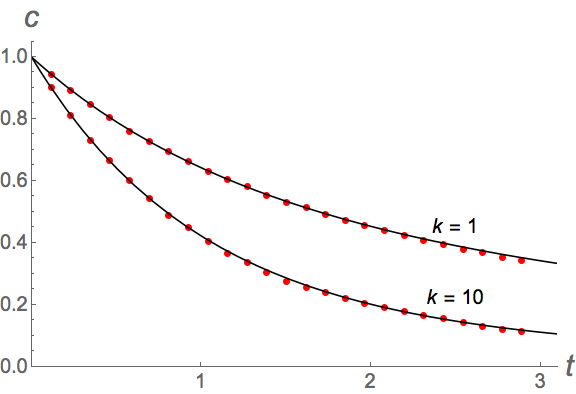
We find similarly good agreement between theory and simulations for coupling scheme (b), as shown in Figure 2.

Figure 2: Decay of the disorder parameter $c(t)$ for coupling scheme (b), which assumes a fixed absorption distance $k/N$. Black curves, theoretical predictions; red dots, simulation results for $N=5000$ oscillators. Plots for $k=1$ and $k=10$ are shown.

Having solved for $c$, we could solve for the individual cluster densities $c_{i}$ and the moments $M_{i}$. Nothing qualitatively new happens (compared to what we saw in the main text for the original model), so we omit the details.

II Fictional Firefly Oscillators

The Scrambler model is a toy model. We introduced it to give the simplest possible mean-field model of pulse-coupled oscillators. Specifically, it was the random shuffling of oscillators during each firing event that simplified their analysis. It conveniently kept the voltages of all oscillators (and all clusters of oscillators) uniformly distributed on $[0,1]$ at all times.

The extreme randomness of this resetting rule, however, is contrived. Traditional models of pulse-coupled oscillators, such as those analyzed by Peskin Peskin (1975) and Mirollo and Strogatz Mirollo and Strogatz (1990), obey deterministic resetting rules, much as real biological oscillators obey deterministic phase-response curves Winfree (2001). As we will show below, models with deterministic resetting can be reasonably approximated within the framework developed here.

For simplicity, we will restrict attention to an almost absurdly idealized model of pulse-coupled oscillators, even more idealized than the models discussed in Refs. Peskin (1975); Mirollo and Strogatz (1990). It consists of what we will refer to as Firefly oscillators. (Fictional Firefly oscillators would be a more apt description, given that essentially everything about the model is unrealistic for real fireflies.)

II.1 Fireflies vs. Scramblers

The equations of motion for the Fireflies are the same as for the Scramblers: $\dot{x_{i}}=1$ (in between firing events). The initial voltages are again drawn from a uniform distribution. However, when a cluster of $j$ synchronized Fireflies reaches the threshold value of 1, that cluster does just two things: (i) it imparts a voltage pulse of size $j/N$ to all other oscillators. Any subsequent oscillators that reach threshold by virtue of this extra $j/N$, and hence get absorbed by the firing cluster, do not fire until the next time they reach threshold. As before, this is to avoid complications that would be caused by chain reactions of firings. (ii) The cluster resets to $x=0$ along with any oscillators it absorbed.

Will the Fireflies behave like the Scramblers? One difference between them has to do with how their speed $\dot{x}$ evolves as the system moves toward complete synchrony. The average speed of the Fireflies doesn’t remain constant at unity, as it does for the Scramblers. This is because when a cluster of size $j$ fires, all the other oscillators receive a pulse of size $j/N$ which boosts them up on their voltage curve (whereas the Scramblers were just randomly reassigned on $[0,1]$, and so keep the same speed $v_{i}=1$ on average). The speeds of the Scramblers are thus $v_{i}=1+v_{\mathrm{pulse}}$, where $v_{\mathrm{pulse}}$ must be determined.

A second difference is that the firing rate of the Fireflies is piecewise constant (unlike that of the Scramblers, which as shown in the main text is a continuous function of time: $R_{i}(t)=c_{i}(t)/2$.) To see why the firing rate for the Fireflies is piecewise constant, first define $\Delta x_{i}$ as the distance between the $i^{th}$ and $(i+1)^{th}$ oscillators (or cluster of synchronized oscillators). Second, divide the temporal evolution into periods $\{T_{n}\}$, where each period is the time taken for the full population to complete a full cycle. Then ask, how does $\Delta x_{i}$ behave during the first period, the time taken for the first wave of oscillators to complete their first cycle? Since all oscillators receive the same number of pulses and have the same speed, we see that each $\Delta x_{i}$ won’t change while the oscillators complete their virgin ascent through [0,1]. This implies a constant firing rate during this first period.

We will later show that this is not unique to the first period: the firing rates will take different, but constant, values during each period; they will be piecewise constant. This is in stark contrast to the Scramblers, where each $\Delta x_{i}$ is constantly changing as the oscillators get reshuffled on $[0,1]$ during each firing event.

II.2 Intuitive Picture of the Dynamics

With these differences in mind, we begin with a qualitative description of the dynamics. As mentioned, the speed of each oscillator, and the effect of a pulse on each oscillator, is the same. This means that the initial ordering of oscillators, or clusters of oscillators, will be invariant throughout the dynamics. They all march forward through $[0,1]$ in a line with no passing.

Then we consider the average behavior as $N\rightarrow\infty$. In this limit, the average spacing between oscillators $\langle\Delta x_{i}\rangle$ approaches $N^{-1}$. Now, what happens when the first oscillator fires? It captures all oscillators on the interval $[1-1/N,1)$. Since $\langle\Delta x_{i}\rangle=N^{-1}$, there will be exactly one oscillator on this interval. So, on average, one oscillator will be captured. This procedure will repeat itself for the next oscillator that fires, and the oscillator after that, such that every oscillator that fires captures the one behind itself. In this mean-field sense, then, the first wave of oscillators will be an orderly sequence of fire/capture/fire/capture, so that at the end of the first period, all oscillators will have synchronized into pairs spaced equally apart.

Of course, $\Delta x_{i}$ will have fluctuations about the mean value of $N^{-1}$. For the oscillators spaced such that $\Delta x_{i}<N^{-1}$, no captures will take place. For $\Delta x_{i}>N^{-1}$, at least one capture will take place, and possibly more. So, at $t=T_{1}$ there will be a number of clusters of different sizes. It is not clear how these clusters are distributed on $[0,1]$. Say, for example, that mostly clusters of size $2$ and $3$ formed, while a cluster of size 4 was the first capture, and a cluster of size 6 was the last capture. Then the clusters of sizes 2 and 3 will be approximately uniformly distributed in voltage, while the distribution of those of sizes 4 and 6 will be more sharply peaked.

Nevertheless we assume that the clusters of size $i$ are uniformly distributed on $[0,1]$ for each $i$. We recognize that this won’t be accurate for each $i$ for all values of $t$. It will however be accurate for those values of $i$ which contain most of the oscillator “mass” and less so for those with less of the mass. So, our assumption will be imprecise for those $c_{i}$ which are small, but since they are small, the inaccuracy won’t matter, to first order.

Now that we understand the first period, how will the second period proceed? We again consider the average behavior as $N\rightarrow\infty$. In this mean-field description, we earlier concluded that at the end of the first period, all oscillators would have synchronized into pairs spaced equally apart on $[0,1]$. When the first pair fires, therefore, there will again be exactly one pair of synchronized oscillators behind them, and so as before, the second period will be an orderly sequence of fire/capture/fire/capture, resulting in all oscillators having synchronized into clusters of size 4.

Continuing this logic, we see the size of clusters will double during each period. Moreover, we observed that the clusters of oscillators will begin each period evenly spaced from each other. This implies the aforementioned piecewise constant firing rate. The mean-field dynamics are therefore trivial: there is a train-like progression of clusters of the same size through $[0,1]$, with each cluster that reaches threshold doubling in size by absorbing the cluster behind it.

II.3 Mean-Field Analysis

With this picture in mind, we analyze the rate equation for our disorder parameter: $\dot{c}=-\sum_{i}R_{i}L_{i}$.

To calculate $L_{i}$, we again find all oscillators in the interval $[1-i/N,1)$. It is tempting to write down $L_{i}(t)=\sum_{j}(i/N)N_{j}(t)$. This isn’t strictly true however, because as we observed, $\Delta x_{i}$ will be constant during each period, which means we must evaluate $N_{j}$ at the start of said period. To make this clear, define $\tilde{x}(t)=x(t=T_{n-1})$ for $T_{n-1}<t<T_{n}$. The tilde notation signifies that throughout the $n^{th}$ period the quantity $x$ is fixed at its value at the start of that period. In terms of this tilde notation, the desired result is $L_{i}=\sum_{j}(i/N)\tilde{N_{j}}(t)=i\tilde{c}$.

To find the firing rate, we follow the procedure used in the main text for the Scramblers: we decompose the firing rate into two parts: $R_{i}=R_{i}^{0}-R_{i}^{a}$. The rate of firing in the absence of absorption will be $R_{i}^{0}=\tilde{c_{i}}v_{i}=\tilde{c_{i}}(1+v_{\mathrm{pulse}})$. The absorption rate will again be $R_{i}^{a}=\sum_{j}(j/N)\tilde{N_{i}}R_{j}=\tilde{c_{i}}\sum_{j}jR_{j}$.

We next determine $v_{\mathrm{pulse}}$. The “pulse velocity” due to a cluster of size $j$ will be (absolute number of pulses per sec) $\times$ (distance per pulse). Since $R_{j}$ is the rate of firing of $c_{i}$, $R_{j}N$ will give the absolute number of fires. The distance per pulse is $j/N$. The total pulse velocity is thus $v_{\mathrm{pulse}}=\sum_{j}(NR_{j})(j/N)=\sum_{j}jR_{j}$. This gives $R_{i}^{0}=\tilde{c_{i}}(1+\sum_{j}jR_{j})$. Putting all this together, we find R_i = ~c_i(1 + ∑_j j R_j) - ~c_i ∑_j j R_j
which reduces to $R_{i}=\tilde{c_{i}}$. Substituting our expressions for $R_{i}$ and $L_{i}$ into the rate equation for $c$ then yields ˙c &= - ∑_i L_i R_i = - ∑_i i ~c ~c_i = - ~c ∑_i i ~c_i= - ~c
and hence $\dot{c}=-\tilde{c}.$ Thus, we see that $\dot{c}$ will be a piecewise linear function. To solve for this function, we need to determine the periods $\{T_{n}\}$. The average speed is $v=1+v_{\mathrm{pulse}}=1+\sum_{j}jR_{j}=1+\sum_{j}jc_{j}=2$. This gives $\{T_{n}\}=\{0,0.5,1,\dots\}$. For these values of $\{T_{n}\}$ and the initial condition $c(0)=1$, the solution of Eq. (II.3) is the piecewise linear function c(t) = p+2-2t2p+1,           p2 ¡ t ¡ p+12 where $p=0,1,2,\dots$. Hence, for the Firefly model, the disorder parameter $c(t)$ is a series of line segments of length $0.5$, with slopes that are sequentially reduced by a factor of 2.

Figure 3: Piecewise linear behavior of the disorder parameter $c(t)$ for the Firefly model. Black curve, theoretical prediction (II.3); red dots, simulation results for $N=5000$ oscillators.

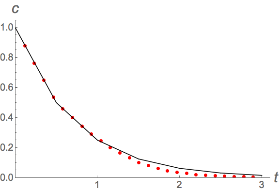
We stress however that our results for $L_{i},R_{i},v_{\mathrm{pulse}}$, and $c(t)$ are only leading-order approximations, based on mean-field arguments. We expect fluctuations around these values. Our hope is that these will be small. Figure 3 shows the simulated behavior of $c(t)$ against the mean-field prediction (II.3). As can be seen, there is reasonable agreement until late times. Now that we have $c(t)$, the next target is $c_{i}(t)$. Carrying out the same analysis as for the Scramblers, we find ˙c_i = - 2~c_i + ∑_k=1^i ~c_k   e^-k ~c ∑_∑p a_p = i-k ( ∏_p ≥1 (k ~cp)apap! ).
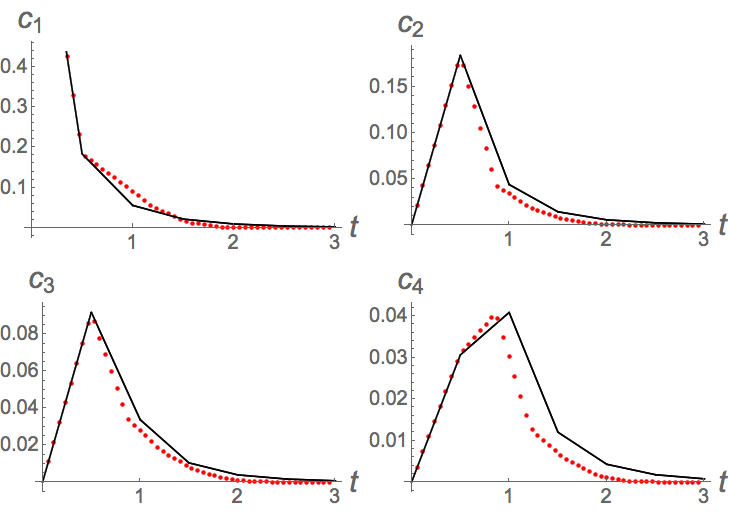
Since the quantities on the right hand side are held fixed over each period, solving for each $c_{i}$ is straightforward. Figure 4 shows the resulting solutions along with simulated values. Reasonable agreement is evident. We restate that our results are mean-field equations, so some discrepancy is expected. The moments $M_{i}(t)$ will also be piecewise linear, and can be obtained in a similarly straightforward manner, following the methods shown in the main text.

Figure 4: Time evolution of the cluster densities $c_{1}$ through $c_{4}$ for the Firefly model with uniformly random initial conditions. Black curves, theoretical predictions derived from Eq. (II.3); red dots; simulation results for for $N=3\times 10^{4}$ oscillators. The discrepancies are due to finite-$N$ effects.

References

- Peskin (1975) C. S. Peskin, Mathematical Aspects of Heart Physiology (Courant Institute of Mathematical Sciences, New York, 1975), pp. 268–278.
- Mirollo and Strogatz (1990) R. E. Mirollo and S. H. Strogatz, SIAM Journal on Applied Mathematics 50, 1645 (1990).
- Winfree (2001) A. T. Winfree, The Geometry of Biological Time (Springer, New York, 2001).