A Precise Determination of from the C-parameter Distribution
Abstract
We present a global fit for , analyzing the available C-parameter data measured at center-of-mass energies between and GeV. The experimental data is compared to a N3LL′ + + theoretical prediction (up to the missing four-loop cusp anomalous dimension), which includes power corrections coming from a field theoretical nonperturbative soft function. The dominant hadronic parameter is its first moment , which is defined in a scheme which eliminates the renormalon ambiguity. The resummation region plays a dominant role in the C-parameter spectrum, and in this region a fit for and is sufficient. We find and with for bins of data. These results agree with the prediction of universality for between thrust and C-parameter within 1-.
I Introduction
In order to study Quantum Chromodynamics (QCD) accurately in the high-energy regime, it is useful to exploit the wealth of data from previous colliders such as LEP. Here the final states coming from the underlying partons created in the collisions appear as boosted and collimated groups of hadrons known as jets. Event shapes have proven to be very successful to study these collisions quantitatively. They combine the energy and momenta of all of the measured hadrons into an infrared- and collinear-safe parameter which describes the geometric properties of the whole event by a single variable distribution. Due to their global nature event shapes have nice theoretical properties, making it possible to obtain very accurate theoretical predictions using QCD. Most event shape variables quantify how well the event resembles the situation of two narrow back-to-back jets, called dijets, by vanishing in this limit. Because the dijet limit involves restrictions that only allow collinear and soft degrees of freedom for the final-state radiation, such QCD predictions involve a number of theoretical aspects that go beyond the calculation of higher-order perturbative loop corrections. These include factorization, to systematically account for perturbative and nonperturbative contributions, and the resummation of large logarithmic corrections by renormalization group evolution. Comparisons of predictions for event shapes with experimental data thus provide non-trivial tests of the dynamics of QCD.
Due to the high sensitivity of event shapes to jets induced by gluon radiation they are an excellent tool to measure the strong coupling . For more inclusive hadronic cross sections (like hadrons) the dependence is subleading because it only occurs in corrections to a leading order term, while for event shapes the dependence is a leading-order effect. For this reason, the study of event shapes for determining has a long history in the literature (see the review Kluth (2006) and the workshop proceedings Bethke (2013)), including recent analyses which include higher-order resummation and corrections up to Gehrmann-De Ridder et al. (2007a); Davison and Webber (2009); Becher and Schwartz (2008); Dissertori et al. (2010); Gehrmann-De Ridder et al. (2009); Chien and Schwartz (2010); Abbate et al. (2011, 2012); Gehrmann et al. (2013); Hoang et al. (2014).
Several previous high-precision studies which determine Davison and Webber (2009); Becher and Schwartz (2008); Abbate et al. (2011, 2012); Gehrmann et al. (2013) focus on the event shape called thrust Farhi (1977),
| (1) |
where is called the thrust axis and it follows from the above equation that . Another event shape, known as C-parameter Parisi (1978); Donoghue et al. (1979), can be written as:
| (2) |
where gives the angle between particles and . It is straightforward to show that . In a previous paper Hoang et al. (2014) we computed the C-parameter distribution with a resummation of large logarithms at N3LL′ accuracy, including fixed-order terms up to and hadronization effects using a field-theoretic nonperturbative soft function. These results were achieved by using the Soft Collinear Effective Theory (SCET) Bauer et al. (2001a, b); Bauer and Stewart (2001); Bauer et al. (2002a, b). Our results for are valid in all three of the peak, tail, and far-tail regions of the distribution, and are the most accurate predictions available in the literature, having a perturbative uncertainty of at for the region relevant for and fits. The same accuracy was previously achieved for thrust, where the remaining perturbative uncertainty in the distribution is in this region Abbate et al. (2011). In this paper we make use of these new C-parameter theoretical results Hoang et al. (2014) to carry out a global fit to all available data, comparing the results with the analogous global fit for thrust Abbate et al. (2011) where appropriate.
Since both and vanish in the dijet limit, it is worthwhile to contrast them in order to anticipate differences that will appear in the analysis. Differences between and include the following:
-
a)
calculating requires identifying the thrust axis with a minimization procedure, while does not involve a minimization;
-
b)
has a single sum over particles while has a double sum;
-
c)
the size of the nonperturbative region, where the entire shape function is important, is larger for compared to due to an enhancement by a factor of ;
-
d)
the resummation region for is larger than that for thrust since the logarithms appear as compared to , which increases the range of values that are useful for fits;
-
e)
fixed-order predictions for the thrust cross section are smooth across the threshold where non-planar events first contribute, , while the fixed-order C-parameter cross section has an integrable singularity at this threshold, . The singularity for comes from the fact that the leading-order distribution is not continuous at . (The -distribution can be made smooth here using LL resummation Catani and Webber (1997).)
A key similarity is that in the dijet limit () the partonic cross sections for thrust and C-parameter are related up to NLL by using Catani and Webber (1998). This relation quantifies several qualitative relations between and in the dijet region.
Recent higher-order event-shape analyses Davison and Webber (2009); Abbate et al. (2011); Gehrmann et al. (2013); Abbate et al. (2012); Gehrmann et al. (2013) have found values of significantly lower than the world average of Olive et al. (2014) which is dominated by the lattice QCD determination Chakraborty et al. (2015). This includes the determination carried out for thrust at N3LL+ in Ref. Abbate et al. (2011)111Note that results at N3LL require the currently unknown QCD four-loop cusp anomalous, but conservative estimates show that this has a negligible impact on the perturbative uncertainties. Results at N3LL′ also technically require the unknown 3-loop non-logarithmic constants for the jet and soft functions which are also varied when determining our uncertainties, but these parameters turn out to only impact the peak region which is outside the range of our fits in the resummation region., which is also consistent with analyses at N2LL + Gehrmann et al. (2010a, 2013) which consider the resummation of logs at one lower order. In Ref. Banfi et al. (2014) a framework for a numerical code with N2LL precision for many event shapes was found, which could also be utilized for fits in the future. In Ref. Abbate et al. (2011) it was pointed out that including a proper fit to power corrections for thrust causes a significant negative shift to the value obtained for , and this was also confirmed by subsequent analyses Gehrmann et al. (2013). Recent results for from decays Boito et al. (2015), DIS data Alekhin et al. (2012), the static potential for quarks Bazavov et al. (2014), as well as global PDF fits Ball et al. (2012); Martin et al. (2009) also find values below the world average. With the new analysis we present here, we provide another event-shape determination of with a high level of precision. We will also simultaneously examine the leading power correction to the distribution, which should be universal between thrust and C-parameter.
This paper is organized as follows. In Sec. II we review the theoretical calculation of the C-parameter cross section, presented in more detail in Ref. Hoang et al. (2014). The details on the experimental data and fit procedure used in our analysis are given in Secs. III and IV. In Sec. V we present the results of our fit for and the first moment of the nonperturbative soft function, . Fits which include hadron-mass effects are discussed in Sec. V.5. In Sec. VI we make predictions for the peak and far-tail regions of the distribution, which are not used in our fit, and compare those regions to experimental data. The universality of is discussed in Sec VII, where we compare our results with the previous fit done using thrust in Ref. Abbate et al. (2011). Finally, Sec. VIII contains our conclusions. We also include three appendices. The first, Appendix A, contains the formulae needed to calculate the profile functions, the second Appendix B contains results that support our choice for the definition of the renormalon free parameter to use for ; and the third compares fit results for thrust with our profiles and those from Ref. Abbate et al. (2011).
II Theory Review
Until a few years ago, the theoretical uncertainties related to perturbative contributions as well as hadronic power corrections were still larger than the experimental uncertainties. The situation on the theory side has dramatically changed with the calculation of corrections Gehrmann-De Ridder et al. (2007a, b, 2009); Gehrmann-De Ridder et al. (2014); Weinzierl (2008, 2009), and the pioneering use of SCET to obtain higher-order perturbative corrections in Ref. Becher and Schwartz (2008), and to obtain accurate predictions for the full spectrum and a precision description of power corrections in Ref. Abbate et al. (2011). In this section we review the theoretical work behind our calculation of , presented in Ref. Hoang et al. (2014).
SCET separates the physics occurring at the different energy and momentum scales relevant to the underlying jets whose properties are characterized by an event shape. For the C-parameter distribution the relevant scales are: (i) the hard scale , which is related to the production of partons at short distances and is of the order of the center-of-mass energy ; (ii) the jet scale , which governs the formation and evolution of the jets; and (iii) the soft scale , which is the scale of large-angle soft radiation. All three scales are widely separated in the dijet region , where most of the events occur and where the distribution is maximal. There is one function associated to each one of these scales in the factorization theorem that describes the dominant contribution of the C-parameter distribution in the dijet limit: (i) the hard function (the modulus squared of the QCD-to-SCET matching coefficient), which is common to all dijet event-shape factorization theorems; (ii) the jet function (given by matrix elements of quark fields with collinear Wilson lines), which is common for C-parameter Hoang et al. (2014), thrust Abbate et al. (2011) and Heavy-Jet-Mass () Chien and Schwartz (2010); and (iii) the soft function (defined by a vacuum matrix element of purely soft Wilson lines), which in general depends on the specific form of the event shape. Whereas the former two are perturbative (), permitting the calculation of the hard and jet functions as an expansion in powers of , the soft function has perturbative corrections () as well as nonperturbative contributions that need to be accounted for (). Renormalization evolution between the three scales , , and sums up large logarithms to all orders in perturbation theory. It turns out that the soft function anomalous dimension for and are identical Hoang et al. (2014), providing a connection between these two event shapes at every order of perturbation theory. Only corrections related to non-logarithmic terms in their soft functions, and the associated towers of logarithms, differ between and .
The soft function can be further factorized into a partonic soft function , calculable in perturbation theory, and a nonperturbative shape function , which has to be obtained from fits to data. In the strict scheme this factorization was achieved in Refs. Hoang and Stewart (2008); Ligeti et al. (2008). (Analytic power corrections for the C-parameter distributions have also been studied in other schemes and frameworks, see e.g. Refs. Gardi and Magnea (2003); Korchemsky and Tafat (2000); Dokshitzer and Webber (1995).)
The treatment of hadronic power corrections greatly simplifies in the tail of the distribution, defined by , where the shape function can be expanded in an OPE. Here the leading power correction is parametrized by , the first moment of the shape function. The main effect of this leading power correction is a shift of the cross section, . Interestingly, this matrix element is related to the corresponding one in thrust by
| (3) |
This relation was first derived using dispersive models with a single soft-gluon approximation in Ref. Dokshitzer and Webber (1995). The equality can actually be derived to all orders in QCD just using quantum field theory Lee and Sterman (2007), but ignoring hadron-mass effects Salam and Wicke (2001). These hadron-mass effects can also be formulated purely with quantum field theory operators Mateu et al. (2013). Although they may in general give large corrections, hadron-mass effects turn out to violate Eq. (3) at only the level, which is well below the 15% level determination of that we will achieve here. When presenting the results of our fits, we parametrize the power correction using defined in Eq. (3) to ease comparison with our previous analysis which determined this based on thrust Abbate et al. (2011, 2012).
II.1 Factorized Cross Section Formula
In order to understand the perturbative components of the C-parameter cross section we make use of the C-parameter factorization formula. To make the connection to thrust simpler we will often use functions defined with the variable . For the perturbative cross section we find Hoang et al. (2014):
| (4) |
Here is the thrust jet function, obtained by the convolution of the two hemisphere jet functions, . describes the collinear radiation in the direction of the two jets. Its definition and expression up to Lunghi et al. (2003); Bauer and Manohar (2004); Becher and Neubert (2006) can be found in Refs. Becher and Schwartz (2008); Abbate et al. (2011). The three-loop non-logarithmic coefficient of this jet function, , is not known, and we vary it in our scans. The anomalous dimension of is known at three loops, and can be obtained from Ref. Moch et al. (2004).
The hard factor contains short-distance QCD effects and is obtained from the Wilson coefficient of the QCD-SCET matching of the vector and axial-vector currents. The hard function is the same for all event shapes for massless quarks, and its expression up to Matsuura and van Neerven (1988); Matsuura et al. (1989); Gehrmann et al. (2005); Moch et al. (2005); Lee et al. (2010); Baikov et al. (2009); Lee et al. (2010); Gehrmann et al. (2010b), can be found in Ref. Abbate et al. (2011). The full anomalous dimension of is known at three loops, van Neerven (1986); Matsuura et al. (1989); Moch et al. (2005).
The soft function describes wide-angle soft radiation between the two jets. It is defined as
| (5) |
where is an operator whose eigenvalues on physical states correspond to the value of C-parameter for that state: . Since the hard and jet functions are the same as for thrust, the anomalous dimension of the soft function has to coincide with the anomalous dimension of the thrust soft function. Hence one only needs to determine the non-logarithmic terms of the C-parameter soft function. In Ref. Hoang et al. (2014) we computed it analytically at one loop, , and used EVENT2 to numerically determine the two-loop non-logarithmic coefficient , with the result
| (6) |
The three-loop non-logarithmic coefficient of the C-parameter soft function, , is currently not known, and we estimate it with a Padé approximation, assigning a very conservative uncertainty. We vary this constant in our scan analysis. The precise definitions of and as well as can be found in Eqs. (A10) and (A12) of Ref. Hoang et al. (2014).
In Eq. (4) the hard, jet and soft functions are evaluated at a common scale . If fixed-order expressions are used for these functions, then there is no scale choice that simultaneously minimizes the logarithms for these three functions. One can instead renormalization-group evolve from to the respective scales , and at which the logs in each of , , and are minimized, and only use fixed-order expressions for these functions at these scales. In this way, large logs of ratios of the scales are summed up in the renormalization group evolution kernels , , and :
| (7) | ||||
The evolution kernels , and resum the large logarithms, , and explicit expressions can be found in Ref. Hoang et al. (2014). The only unknown piece in our resummation of logarithms at N3LL order is the small contribution from the four-loop cusp anomalous dimension, , which we estimate using a Padé approximation and conservatively vary in our analysis.
While Eq. (7) gives the part of the cross section that is singular and non-integrable as , we also need to include the integrable or nonsingular contribution. This can be written as
| (8) | ||||
The functions , , and were determined in Ref. Hoang et al. (2014) using the fixed-order results at Ellis et al. (1980, 1981); Catani and Seymour (1996, 1997); Gehrmann-De Ridder et al. (2007a, b, 2009); Gehrmann-De Ridder et al. (2014); Weinzierl (2008, 2009). The nonsingular cross section is independent of the renormalization scale order by order, and therefore we evaluate these pieces at the nonsingular scale , and vary this scale to estimate higher-order perturbative nonsingular corrections. The scale variation of will be discussed further in Section II.2.
The full partonic cross section is then given by
| (9) |
Nonperturbative effects are included by convolving Eq. (9) with a shape function:
| (10) |
One important property of this shape function is that its first moment encodes the leading power correction to our cross section. In the scheme this moment is given by
| (11) |
Up to the normalization factors shown in Eq. (3) we expect approximate universality between the for C-parameter and thrust. For the calculation of the cross section, the shape function is expanded in a complete basis of functions obtained by an appropriate infinite-range mapping of the Legendre polynomials Ligeti et al. (2008), with the coefficients chosen to maintain the first moment. For further details on the implementation of the shape function for C-parameter see Ref. Hoang et al. (2014). We remove an renormalon by using the Rgap scheme Hoang and Kluth (2008); Hoang et al. (2010), which introduces a subtraction scale into our formula, as well as the gap parameter and the perturbative scheme-change gap parameter . Here, is given by a perturbative series in whose mass dimension is set by an overall factor of , and which also contains factors. The convolution with the shape function now becomes,
| (12) | ||||
The final component of our cross section is properly accounting for hadron-mass effects following Ref. Mateu et al. (2013). Hadron-mass effects induce an additional series of large perturbative logarithms which start at NLL, , and also break the exact universality between and given in Eq. (3). These effects are accounted for by including dependence on the transverse velocity, , in the nonperturbative matrix elements (here, gives the non-zero hadron mass). In particular, in the Rgap scheme the first moment of the shape function is actually given by
| (13) | ||||
In the scheme the definition accounting for hadron-mass effects is the same as Eq. (13), but one sets and removes as an argument for these parameters. Accounting for both the the running due to hadron masses and the R-evolution running in the Rgap scheme, the evolution of the integrand on the right-hand side of Eq. (13) is given by,
| (14) |
where and give the initial scales where the function is defined. The perturbative evolution kernel gives the and running for each value of . The function encodes the event-shape dependence of the hadron-mass effects and gives the solution to the one-loop RGE for with hadron masses derived in Ref. Mateu et al. (2013). Since the two- and three-loop -dependent anomalous dimensions are unknown, we do not treat the logs generated by hadron-mass effects to the same level of precision. When hadron-mass effects are accounted for we always sum the associated logarithms at NLL. An analogous formula to Eq. (II.1) also holds for the thrust parameter .
Combining all of these elements gives the complete cross section. Note that we can resum to any order up to N3LL′ and can choose to include or leave out the shape function, renormalon subtraction and hadron-mass effects. This flexibility allows us to see how the analysis changes when we take into account each of these additional physical considerations and enables us to test how robust the fits are to various changes in the theoretical treatment.
II.2 Profile Functions
In order to smoothly transition between the nonperturbative, resummation, and fixed-order regions we make use of profile functions for the renormalization scales , , , , and . In the three regions, the requirements on the scales which properly deal with large logarithms, nonperturbative effects, and the cancellations between singular and nonsingular contributions in the fixed-order region are
| (15) | ||||
In addition we take the fixed-order nonsingular scale in the nonperturbative and resummation regions. Our profile functions satisfy these constraints, and provide continuous and smooth transitions between these regions. The resummed perturbative cross section is independent of variations in all renormalization scales order by order in the logarithmic resummation. Therefore the dependence on parameters appearing in the profile functions gets systematically smaller as we go to higher orders, and their variation provides us with a method of assessing perturbative uncertainties.
For the hard renormalization scale we use the -independent formula
| (16) |
where is a parameter that we vary from to in order to account for theory uncertainties.
The soft scale has different functional dependence in the three regions of Eq. (II.2), and hence depends on the following parameters:
| (17) |
Here, controls the intercept of the soft scale at , is near the boundary of the purely nonperturbative region and controls the end of this transition, where the resummation region begins. The transition from nonperturbative to perturbative is dependent, so we use the -independent parameters GeV) and GeV). In the resummation region the parameter determines the slope of the soft scale relative to the canonical resummation region scaling, with . The parameter controls where the transition occurs between the resummation and fixed-order regions and sets the value of where the renormalization scales all become equal as required in the fixed-order region. For the jet scale we have the dependence
| (18) |
where is a parameter that is varied in our theory scans to slightly modify the natural relation between the scales. The exact functional form for and in Eqs. (17) and (18) is given in Appendix A.
To avoid large logarithms in the soft function subtractions , the scale is chosen to be the same as in the resummation and fixed-order regions. In the nonperturbative region we need to obtain an subtraction that stabilizes the soft function in this region (removing unphysical negative dips that appear in the scheme). This introduces an additional parameter . Therefore we have
| (19) |
The exact functional form for is also given in Appendix A.
For the nonsingular scale , we use the variations
| (20) |
Here the three choices vary in a manner that allows it to have some independence from in the resummation and nonperturbative regions, while still being equal in the fixed-order region (where ). These variations of probe the higher-order fixed-order uncertainty in the nonsingular cross section contribution. In the fixed-order region the variation of alone precisely reproduces the standard fixed-order scale variation.
| parameter | default value | range of values |
| GeV | - | |
| GeV | - | |
| to | ||
| to | ||
| to | ||
| to | ||
| to | ||
| to | ||
| to | ||
| , , | ||
| to | ||
| to | ||
| to | ||
| to | ||
| , , | ||
| , , | ||
| , , | ||
| , , |
| parameter | default value | range of values |
| GeV | - | |
| GeV | - | |
| to | ||
| to | ||
| to | ||
| to | ||
| to | ||
| to | ||
| to | ||
| , , | ||
| to | ||
| to | ||
| , , | ||
| , , |
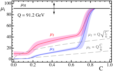
The details of the variations of the profile function parameters used to assess uncertainties are given in Tab. 1. The plot in Fig. 1 shows how the scales vary with the changes to our C-parameter profile parameters. The vertical arrow on the hard scale indicates the overall up/down variation, which causes a variation to all the scales. Also shown (as gray dashed lines) are plots of the canonical soft scale and canonical jet scale . In the resummation region, these correspond fairly well with the profile functions, indicating that in this region our analysis will avoid large logarithms. As discussed in detail in Ref. Hoang et al. (2014), to improve the convergence of the C-parameter cross sections we take as our default slope parameter, explaining why our soft and jet scales are larger than the canonical values in Fig. 1 (by a factor that does not induce further large logs). In the analysis of Sec. V, we will see how varying each of these profile parameters affects our final fit results.
For the numerical analyses carried out in this work we have created within our collaboration two completely independent codes. One code within Mathematica Wolfram Research (2014) implements the theoretical expressions exactly as given in Ref. Hoang et al. (2014), and another code is based on theoretical formulae in Fourier space and realized as a fast Fortran gfo (2014) code suitable for parallelized runs on computer clusters. These two codes agree for the C-parameter distribution at the level of .
We will also repeat the thrust fits of Ref. Abbate et al. (2011), implementing the same type of profile functions used here. These profiles have several advantages over those in Ref. Abbate et al. (2011), including a free variable for the slope, a flat nonperturbative region, and parameters whose impact is much more confined to one of the three regions in Eq. (II.2). For the thrust profiles we redefine , which eliminates the factors of in Eqs. (50) and (56). This way, the canonical choice of slope is for both C-parameter and thrust. We use as our default for thrust as well, again to improve the perturbative convergence, as discussed in Ref. Hoang et al. (2014). The profile parameters for thrust and their variations are summarized in Tab. 2. These choices create profiles that are very similar to those used in Ref. Abbate et al. (2011). The new fit results for thrust are fully compatible with those of Ref. Abbate et al. (2011) in the resummation region used for the fits. Additionally, they give a better description in the nonperturbative region which is outside of our fit range.
II.3 Hadron-mass effects
In Ref. Mateu et al. (2013) it was shown that hadron-mass effects, apart from breaking the universality properties of the leading power correction for various event shapes, also induce a nontrivial running. Since these are single logarithms, they start at NLL order. In Ref. Mateu et al. (2013) the corresponding leading anomalous dimension was determined, which yields the NLL resummation of larger logs between the scales and for a large set of event shapes. The pieces necessary for a higher-order resummation have not yet been computed. One might be worried that accounting for only the NLL running for in an expression as accurate as N3LL in cross-section logs could be inadequate, or that it could leave significant perturbative uncertainties. However, one should recall that the hadronic parameter itself is a correction, and hence it is valid to account for the related resummation with less precision. In this section we show that the evolution at NLL order suffices for the precision of our N3LL analysis. Indeed, it turns out that the effect of the hadron mass running on the fit outcome is very small as compared to other uncertainties, and therefore can be safely neglected.
For our C-parameter analysis the implementation of hadron mass running effects has been explained at length in Ref. Hoang et al. (2014), and we only summarize here the most relevant aspects needed to understand the fit results. In the scheme the leading power correction can be written as an integral of a universal hadron function, , common to all event shapes
| (21) |
where is the transverse velocity, denotes a specific event shape, is a calculable normalization factor, and is an event-shape-dependent function encoding the hadron-mass effects. The functions are known analytically, and specific examples can be found in Ref. Mateu et al. (2013). For C-parameter , while for thrust . For the simple case of the scheme the running between the initial reference scale where the universal hadron function is specified, and the soft scale , is given at leading order by
| (22) |
with . The corresponding evolution formula for the Rgap scheme is considerably more complex, as shown by the form displayed in Eq. (II.1) above. Ensuring that the renormalon is not reintroduced by the renormalization group evolution requires an additional evolution in the scale , so contains evolution in both the and scales. Also here we have two reference scales and to specify the initial parameter . The full formula for is given in Eq. (67) of Ref. Hoang et al. (2014).
Note that the renormalization group evolution is a function of and takes place independently for each , but the required result for C-parameter or thrust requires an integral over . Due to this integration the functional form that we assume for the initial condition or gets entangled with the perturbative resummation.
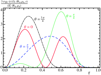
With current constraints on the dependence, and with the lack of even more precise experimental data to probe this issue, a model-independent formulation (like a complete functional basis for the dependence at the reference scales, and ) is not feasible. To implement this running we have therefore tested several models for the dependence in Ref. Hoang et al. (2014), and found that generically the experimental data is sensitive to the normalization which specifies , but not to the detailed form used for the dependence as long as it satisfies several reasonable constraints. Therefore for the fits performed here we simply adopt the default form from Ref. Hoang et al. (2014),
| (23) | ||||
This model ensures that is always positive definite and smoothly goes to zero at the endpoint (where the ratio of the hadron mass to goes to zero). The functions form an orthonormal basis upon integration with , which yields the following relation:
| (24) |
which determines the normalization. We also define
| (25) |
which was chosen to have an effect orthogonal to the more relevant parameter . By examining our ability to simultaneously measure and we have a means to test for the impact that the initial dependence has on our fits. As we can see in Fig. 2, our model captures different behavior for the dependence of by choosing different values of . Over the interval , all the curves in this figure are normalized so that they integrate to .
III Experimental Data
Data on the C-parameter cross section are given by several experiments for a range of from to GeV. We use data from ALEPH 222The ALEPH dataset with GeV has two systematic uncertainties for each bin. The second of these uncertainties is treated as correlated while the first one is treated as an uncorrelated uncertainty and simply added in quadrature to the statistical uncertainty. with , , , , , , , GeV Heister et al. (2004), DELPHI with , , , , , , , , , , , , , , , , GeV Abdallah et al. (2004); Abreu et al. (1997, 1999); Wicke (1999), JADE with , GeV Biebel et al. (1999), L3 with , , , , , , , , , GeV Achard et al. (2004); Adeva et al. (1992), OPAL with , , , GeV Abbiendi et al. (2005), and SLD with GeV Abe et al. (1995). As each of these datasets is given in binned form, our cross section in Eq. (12) is integrated over each bin before being compared to the data. The default range on used in fitting the data is . A lower limit of eliminates the peak region where higher nonperturbative moments become important. The upper limit is chosen to be 0.7 in order to avoid the far-tail region as well as the Sudakov shoulder at . Any bin that contains one of the end points of our range ( or 0.7) is included if more than half of that bin lies within the range. Using the default range and datasets gives a total of bins. As a further test of the stability of our analysis, both this C-parameter range and the selection of datasets is varied in the numerical analysis contained in Sec. V.
In our fitting procedure, we consider both the statistical and systematic experimental uncertainties. The statistical uncertainties can be treated as independent between bins. The systematic experimental uncertainties come from various sources and full documentation of their correlations are not available, so dealing with them in our analysis is more complicated, and we have to use a correlation model. For this purpose we follow the LEP QCD working group Heister et al. (2004); Abbiendi et al. (2005) and use the minimal overlap model. Within one C-parameter dataset, which consists of various C-parameter bins at one value for one experiment, we take for the bin , bin off-diagonal entry of the experimental covariance matrix . Here are the quoted systematic uncertainties of the bins and . Within each dataset, this model implies a positive correlation of systematic uncertainties. In addition to this default model choice, we also do the fits assuming uncorrelated systematic uncertainties, in order to test whether the minimal overlap model introduces any bias. See Sec. V.2 for more details on the correlation matrix.
IV Fit Procedure
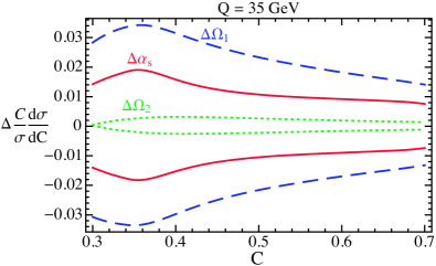
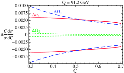
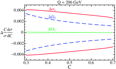
In order to accurately determine both and the leading power correction in the same fit, it is important to perform a global analysis, that is, simultaneously fitting -spectra for a wide range of center-of-mass energies . For each , effects on the cross sections induced by changes in can be partly compensated by changes in , resulting in a fairly strong degeneracy. This is resolved by the global fit, just as in the thrust analysis of Ref. Abbate et al. (2011). Fig. 3 shows the difference between the theoretical prediction for the cross section at three different values of , when or are varied by and GeV, respectively. It is clear that the potential degeneracy in these parameters is broken by having data at multiple values. In Fig. 3 we also vary the higher-order power correction parameter , which clearly has a much smaller effect than the dominant power correction parameter .
To carry out a fit to the experimental data we fix the profile and theory parameters to the values shown in Tab. 1. The default values are used for our primary theory cross section. We integrate the resulting theoretical distribution over the same C-parameter bins as those available experimentally, and construct a function with the uncorrelated statistical experimental uncertainties and correlated systematic uncertainties. This is a function of and , and is very accurately described by a quadratic near its global minimum, which therefore determines the central values and experimental uncertainties. The value of and its associated uncertainties encode the dominant hadronization effect as well as the dominant residual uncertainty from hadronization.
To obtain the perturbative theoretical uncertainty we consider the range of values shown for the theory parameters in Tab. 1. Treating each of these as a flat distribution, we randomly generate values for each of these parameters and then repeat the fit described above with the new function. This random sampling and fit is then repeated 500 times. We then construct the minimum ellipse that fully contains all 500 of the central-fit values by first creating the convex envelope that contains all of these points within it. Then, we find the equation for the ellipse that best fits the points on the envelope, with the additional restrictions that all values lie within the ellipse and its center is the average of the maximum and minimum values in each direction. This ellipse determines the perturbative theoretical uncertainty, which turns out to be the dominant uncertainty in our fit results. In our final results the perturbative and experimental uncertainties are added in quadrature. This procedure is similar to that discussed in the Appendix of Ref. Abbate et al. (2012).
V Results
In this section we discuss the results from our global analysis. We split the presentation into several subsections. In Sec. V.1 we discuss the impact that resummation and the inclusion of power corrections have on the fit results. In Sec. V.2 we present the analysis which yields the perturbative uncertainty in detail, cross-checking our method by analyzing the order-by-order convergence. We also analyze the impact of removing the renormalon. In Sec. V.3 we discuss the experimental uncertainties obtained from the fit. Section V.4 discusses the impact that varying the theory parameters one by one has on the best-fit points, allowing us to determine which parameters dominate the theoretical uncertainty. The impact of hadron-mass resummation is discussed in detail in Sec. V.5. We examine the effects of changing the default dataset in Sec. V.6. The final fit results are collected in Sec. V.7. When indicating the perturbative precision, and whether or not the power correction is included and at what level of precision, we use the following notation:
| fixed order up to | ||||
| perturbative resummation | ||||
| scheme for | ||||
| Rgap scheme for | ||||
| Rgap scheme with | ||||
V.1 Impact of Resummation and Power Corrections
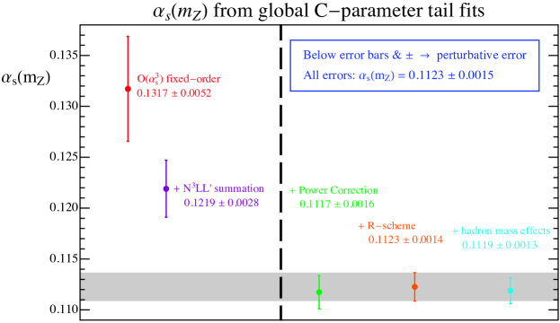
In Fig. 4 we show extracted from fits to the tail of the C-parameter distribution including sequential improvements to the treatment of perturbative and nonperturbative components of our code, using the highest perturbative accuracy at each stage. The sequence from left to right shows the fit results using: fixed-order results only, adding N3LL resummation, adding the power correction, adding renormalon subtractions and using the Rgap power correction parameter , and adding hadron-mass effects. These same results together with the corresponding are also collected in Tab. 3. The fit with only fixed-order results has a relatively large and also its central value has the largest value of . Including the resummation of large logarithms decreases the central by 8% and also decreases the perturbative uncertainty by . Due to this smaller perturbative uncertainty it becomes clear that the theoretical cross section has a different slope than the data, which can be seen, for example, at for . This leads to the increase in the for the “N3LL′ no power corr.” fit, and makes it quite obvious that power corrections are needed. When the power correction parameter is included in the fit, shown by the third entry in Tab. 3 and the result just to the right of the vertical dashed line in Fig. 4, the becomes and this issue is resolved. Furthermore, a reduction by is achieved for the perturbative uncertainty in . This reduction makes sense since some of the perturbative uncertainty of the cross section is now absorbed in , and a much better fit is achieved for any of the variations associated to estimating higher-order corrections. The addition of also caused the fit value of to drop by another 8%, consistent with our expectations for the impact of power corrections and the estimate made in Ref. Hoang et al. (2014). Note that the error bars of the first two purely perturbative determinations, shown at the left-hand side of the vertical thick dashed line in Fig. 4 and in the last two entries in Tab. 3, do not include the uncertainties associated with the lack of power corrections.
The remaining corrections we consider are the use of the R-scheme for which includes the renormalon subtractions, and the inclusion of the log-resummation effects associated to the hadron-mass effects. Both of these corrections have a fairly small impact on the determination of , shifting the central value by and respectively. Since adding the shift from the hadron mass corrections in quadrature with the perturbative uncertainty does not change the overall uncertainty we will use the R-scheme determination for our main result. This avoids the need to fully discuss the extra fit parameter that appears when hadron masses are included. Further discussion of the experimental uncertainties and the perturbative uncertainty from the random scan are given below in Secs. V.2 and V.4, and a more detailed discussion of the impact of hadron-mass resummation is given below in Sec. V.5.
The values of obtained from the fits discussed above can be directly compared to the power correction obtained from the thrust distribution. Values for from the C-parameter fits are given below in Secs. V.2 and V.4 and the comparison with thrust is considered in Sec. VII.
| N3LL′ + hadron | ||
|---|---|---|
| N3LL′ with | ||
| N3LL′ with | ||
| N3LL′ no power corr. | ||
| fixed order no power corr. |
V.2 Perturbative Uncertainty from the Scan
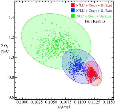
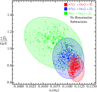
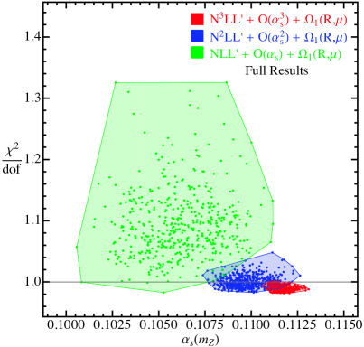
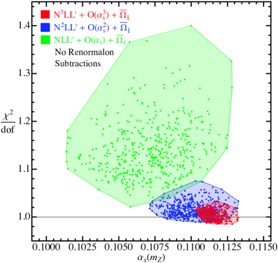
To examine the robustness of our method of determining the perturbative uncertainty by the random scan, we consider the convergence and overlap of the results at different perturbative orders. Figure 5 shows the spread of best-fit values at NLL′, N2LL′ and N3LL′. The upper left panel, Fig. 5, shows results from fits performed in the Rgap scheme, which implements a renormalon subtraction for , and the upper right-panel, Fig. 5, shows results in the scheme without renormalon subtractions. Each point in the plot represents the outcome of a single fit, and different colors correspond to different orders in perturbation theory. Not unexpectedly, fits in the Rgap scheme show generally smaller theory uncertainties.
In order to estimate correlations induced by theoretical uncertainties, each ellipse in the - plane is constructed following the procedure discussed in Sec. IV. Each theory ellipse constructed in this manner is interpreted as an estimate for the 1- theoretical uncertainty ellipse for each individual parameter (39% confidence for the two parameters), and is represented by a dashed ellipse in Fig. 5. The solid lines represent the combined (theoretical plus experimental) standard uncertainty ellipses at 39% confidence for two parameters, obtained by adding the theoretical and experimental error matrices from the individual ellipses, where the experimental ellipse corresponds to . Figure 5 clearly shows a substantial reduction of the perturbative uncertainties when increasing the resummation accuracy, and given that they are 39% confidence regions for two parameters, also show good overlap between the results at different orders.
The results for and from the theory scan at different perturbative orders are collected in Tabs 4 and 5. Central values here are determined from the average of the maximal and minimal values of the theory scan, and are very close to the central values obtained when running with our default parameters. The quoted perturbative uncertainties are one-parameter uncertainties.
| order | (with ) | (with ) |
|---|---|---|
| NLL′ | ||
| N2LL′ | ||
| N3LL′ (full) |
| order | [GeV] | [GeV] |
|---|---|---|
| NLL′ | ||
| N2LL′ | ||
| N3LL′ (full) |
In Tab. 3 above we also present results with no power corrections and either using resummation or fixed-order perturbative results. Without power corrections there is no fit for , so we take the central value to be the average of the maximum and minimum value of that comes from our parameter scan. Our estimate of the uncertainty is given by the difference between our result and the maximum fit value. For the fixed-order case, since there is only one renormalization scale, we know that the uncertainties from our parameter variation for , , and are uncorrelated. So, we take the fit value for with the default parameters as our result and add the uncertainties from variations of these parameter in quadrature to give the total uncertainty.
An additional attractive result of our fits is that the experimental data is better described when increasing the order of the resummation and fixed-order terms. This can be seen by looking at the minimal dof values for the best-fit points, which are shown in Fig. 5. In Figs. 5 and 5 we show the distribution of values for the various best-fit points. Figure 5 displays the results in the Rgap scheme, whereas Fig. 5 shows the results in the scheme. In both cases we find that the values systematically decrease with increasing perturbative order. The highest-order analysis in the scheme leads to values around unity and thus provides an adequate description of the whole dataset, however one also observes that accounting for the renormalon subtraction in the Rgap scheme leads to a substantially improved theoretical description having values below unity essentially for all points in the random scan. Computing the average of the values we find at N3LL′ order for the Rgap and schemes and , respectively (where the spread of values is smaller in the Rgap scheme). Likewise for N2LL′ we find and , and for NLL′ we find and . These results show the excellent description of the experimental data for various center-of-mass energies. They also validate the smaller theoretical uncertainties obtained for and at N2LL′ and N3LL′ orders in the Rgap scheme.
V.3 Experimental Fit Uncertainty
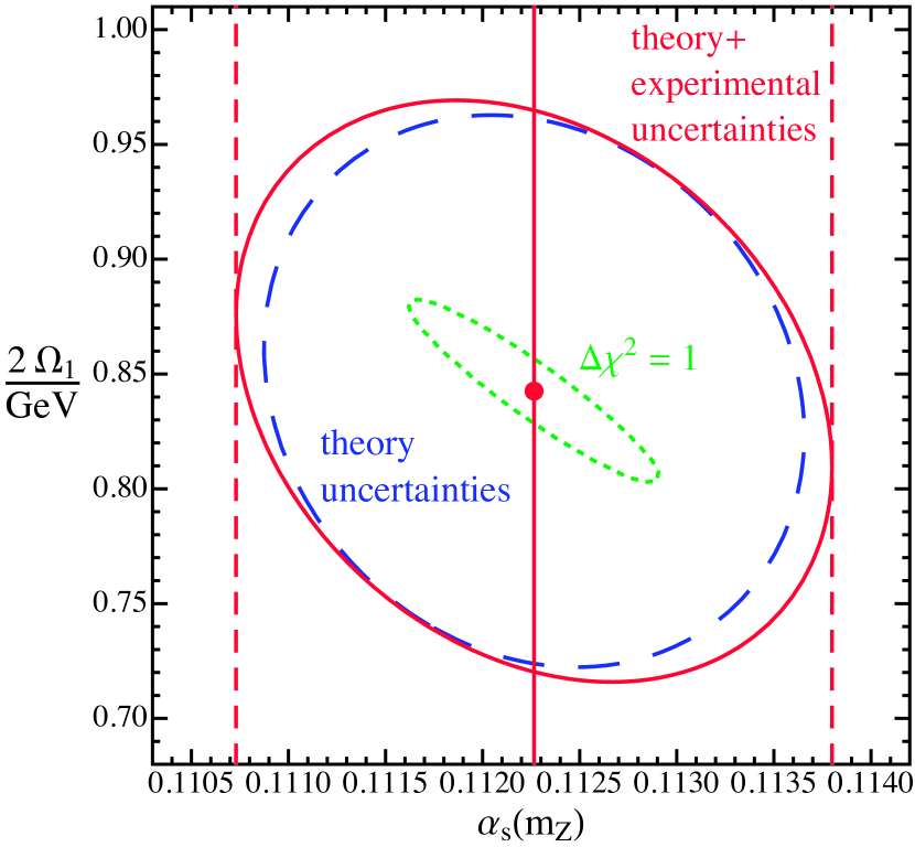
Next we discuss in more detail the experimental uncertainty in and the hadronization parameter as well as the combination with the perturbative uncertainty done to obtain the total uncertainty.
Results are depicted in Fig. 6 for our highest order fit including resummation, power corrections and renormalon subtractions. The inner green dotted ellipse, blue dashed ellipse, and solid red ellipse represent the uncertainty ellipses for the experimental, theoretical, and combined theoretical and experimental uncertainties respectively. These ellipses correspond to the one-dimensional projection of the uncertainties onto either or (39% confidence ellipse for two parameters). The correlation matrix of the experimental, theory, and total uncertainty ellipses are (for ),
| (28) | ||||
| (31) | ||||
| (34) | ||||
| (37) |
Note that the theoretical uncertainties dominate by a significant amount. The experimental correlation coefficient is significant and reads
| (38) |
The theory correlation coefficient is small, , and since these uncertainties dominate it reduces the correlation coefficient for the total uncertainty to
| (39) |
In both Eqs. (38) and (39) the numbers in parentheses indicate a range that captures all values obtained from the theory scan. The correlation exhibited by the green dotted experimental uncertainty ellipse in Fig. 6 is given by the line describing the semimajor axis
| (40) |
Note that extrapolating this correlation to the extreme case where we neglect the nonperturbative corrections () gives which is consistent with the result of our fit without power corrections in Tab. 3.
From in Eq. (28) it is possible to extract the experimental uncertainty for and the uncertainty due to the imprecise determination of ,
| (41) |
and to extract the experimental uncertainty for and its uncertainty due to the imprecise determination of ,
| (42) |
V.4 Individual Theory Scan Errors
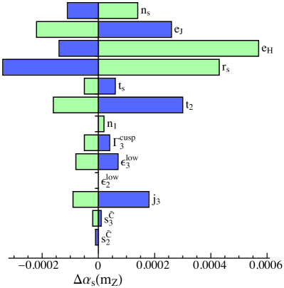
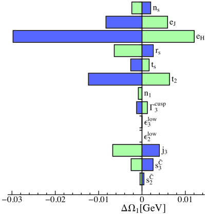
To gain further insight into our theoretical precision and in order to estimate the dominant source for theory uncertainty from missing higher-order terms, we look at the size of the theory uncertainties caused by the individual variation of each one of the theory parameters included in our random scan. In Fig. 7 two bar charts are shown with these results for (left panel) and (right panel) for fits corresponding to our best theoretical setup (with N3LL′ accuracy and in the Rgap scheme). The dark blue bars correspond to the result of the fit with an upward variation of the given parameter from Tab. 1, while the light green bars correspond to the fit result from the downward variation in Tab. 1. Here we vary a single parameter keeping the rest fixed at their default values. We do not show parameters that have a negligibly small impact in the fit region, e.g. and , which only have an effect on the cross section to the right of the shoulder, or , which only affects the cross section in the nonperturbative region.
We see that the dominant theory uncertainties are related to variations of the profile functions (), where is the largest source of uncertainty, and is particularly dominant for . The second most important uncertainty comes from for and for , and also has a significant effect on both parameters.
As expected, the parameters associated to the transitions on the sides of our fit region, and , hardly matter. The renormalization scale parameter for the nonsingular partonic distribution also causes a very small uncertainty since the nonsingular terms are always dominated by the singular terms in our fit region. The uncertainties related to the numerical uncertainties of the perturbative constants (, , ) as well as the numerical uncertainties in the extraction of the nonsingular distribution for small values, (, ) are – with the possible exception of – much smaller and do not play an important role. The uncertainty related to the unknown -loop contribution to the cusp anomalous dimension is always negligible. Adding quadratically the symmetrized individual uncertainties shown in Fig. 7, we find for and GeV for . This is about one half of the theoretical uncertainty we have obtained by the theory parameter scan for (or five sixths for ), demonstrating that incorporating correlated variations through the theory parameter scan represents a more realistic method to estimate the theory uncertainty.
V.5 Effects of hadron-mass resummation
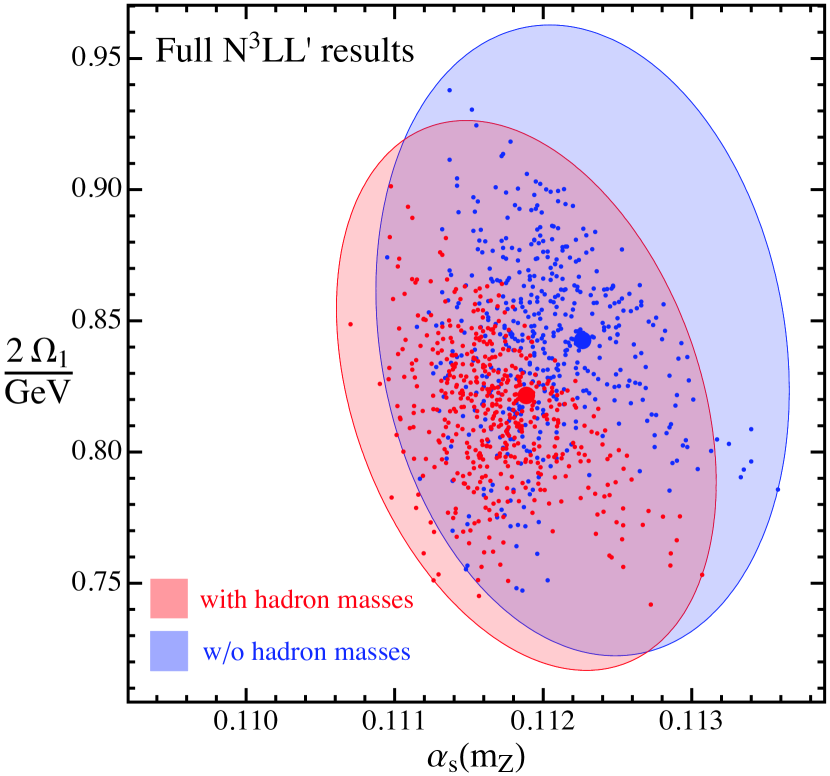
The fit results presented in the previous two sections ignored the small hadron-mass effects. These effects are analyzed in greater detail in this section. We again perform fits for a theory setup which includes N3LL′ accuracy and a power correction in the Rgap scheme, but this time it also includes hadron-mass-induced running.
Since the impact of hadron-mass effects is small, one finds that the experimental data in the tail of the distribution is not accurate enough to fit for in Eq. (25), in addition to and . This is especially true because it enters as a small modification to the power correction, which by itself is not the dominant term. Indeed, fitting for and as defined in Eq. (II.3) gives a strongly correlated determination of these two parameters. The dominant hadronic parameter , which governs the normalization, is still as accurately determined from data as the in Tab. 5. However, the orthogonal parameter is only determined with very large statistical uncertainties. As discussed in Ref. Hoang et al. (2014), the specific value of has a very small impact on the cross section, which is consistent with the inability to accurately fit for it.
The results of our fit including hadron-mass effects are
| (43) | |||
Note that the meaning of here is different from the case in which hadron-mass running effects are ignored because there are extra evolution effects needed to translate this value to that used in the cross section at a given value of , compared to the no-hadron-mass case.
In Fig. 8 we compare the outcome of the fits at N3LL′ in the Rgap scheme. Results with hadron-mass effects give the red ellipse on the left, and without hadron-mass effects give the blue ellipse on the right. (The latter ellipse is the same as the one discussed above in Sec. V.2.) The effects of hadron masses on are to decrease its central value by and reduce the percent perturbative uncertainty by . Given that the total perturbative uncertainties are , these effects are not statistically significant. When studying the effect on one has to keep in mind that its meaning changes when hadron-mass effects are included. Ignoring this fact we observe that hadron masses shift the central value downwards by , and reduce the percent theoretical uncertainty by . Again, given that the perturbative uncertainty for is , this shift is not significant.
Since the theory uncertainties become slightly smaller when hadron-mass effects are incorporated, one could use this setup as our default. However we take a more conservative approach and consider the shift on the central value as an additional source of uncertainty, to be added in quadrature to the hadronization uncertainty already discussed in Sec. V.2. This increases the value of the hadronization uncertainty from to , and does not affect the total uncertainty. The main reason we adopt this more conservative approach is that, while well motivated, the ansatz that we take in Eq. (II.3) is not model independent. We believe that this ansatz serves as a good estimate of what the numerical effect of hadron masses are, but should likely not be used for the central fit until further theoretical insight on the form of is gained. We do not add an additional uncertainty to since hadron-mass effects change its meaning and uncertainties for are large enough that these effects are negligible.
In App. B we also consider fits performed using the Rgap scheme with C-parameter gap subtractions, rather than our default Rgap scheme with thrust gap subtractions. The two results are fully compatible. As discussed in Ref. Hoang et al. (2014) the thrust gap subtractions give better perturbative convergence, and hence are used for our default cross section.
V.6 Dataset dependence
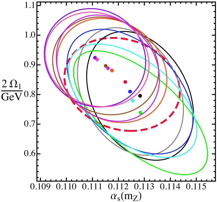
In this section we discuss how much our results depend on the dataset choice. Our default global dataset accounts for all experimental bins for GeV in the intervals , (more details are given in Sec. III). The upper limit in this range is motivated by the fact that we do not want to include data too close to the shoulder, since we do not anticipate having the optimal theoretical description of this region. The lower limit avoids including data too close to the nonperturbative region, which is near the cross section peak for , since we by default only include the leading power correction in the OPE of the shape function. To consider the impact of this dataset choice we can vary the upper and lower limits used to select the data.
In Fig. 9 the best fits and the respective total experimental + theory CL uncertainty ellipses (for two parameters) are shown for global datasets based on different choices of data ranges. The result for our default global dataset is given in red, with a thicker, dashed ellipse. In the caption of Fig. 9 the data ranges and the number of bins are specified for each one of the plotted ellipses.
Interestingly all uncertainty ellipses have very similar correlation and are lined up approximately along the line
| (44) |
As expected, the results of our fits depend only weakly on the range and the size of the global datasets, as shown in Fig. 9. The size and tilt of the total uncertainty ellipses is very similar for all datasets (with the exception of , which clearly includes too much peak data). Since the centers and the sizes of the uncertainty ellipses are fully statistically compatible at the - level, this indicates that our theory uncertainty estimate at N3LL′ really reflects the accuracy at which we are capable of describing the different regions of the spectrum. Therefore a possible additional uncertainty that one could consider due to the arbitrariness of the dataset choice is actually already represented in our final uncertainty estimates.
V.7 Final Results
As our final result for and , obtained at N3LL′ order in the Rgap scheme for , we get
| (45) | ||||
where GeV and we quote individual - uncertainties for each parameter. Here . Equation (45) is the main result of this work.
Equation (45) accounts for the effect of hadron mass running through an additional (essentially negligible) uncertainty. Also, it neglects QED and finite bottom-mass corrections, which were found to be small effects in the corresponding thrust analysis in Ref. Abbate et al. (2011).
Given that we treat the correlation of the systematic experimental uncertainties in the minimal overlap model, it is useful to examine the results obtained when assuming that all systematic experimental uncertainties are uncorrelated. At N3LL′ order in the Rgap scheme the results that are analogous to Eq. (45) read and GeV with a combined correlation coefficient of . The results are compatible with Eq. (45), indicating that the ignorance of the precise correlation of the systematic experimental uncertainties barely affects the outcome of the fit.
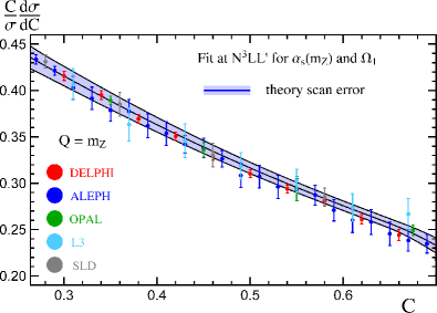
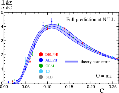
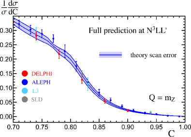
In Fig. 10 we show the theoretical fit for the C-parameter distribution in the tail region, at a center-of-mass energy corresponding to the -pole. We use the best-fit values given in Eq. (45). The band corresponds to the perturbative uncertainty as determined by the scan. The fit result is shown in comparison with experimental data from DELPHI, ALEPH, OPAL, L3 and SLD. Good agreement is observed for this spectrum, as well as for spectra at other center of mass values.
VI Peak and Far Tail Predictions
Even though our fits were performed in the resummation region which is dominated by tail data, our theoretical results also apply for the peak and far-tail regions. As an additional validation for the results of our global analysis in the tail region, we use the best-fit values obtained for and to make predictions in the peak and the far-tail regions where the corresponding data was not included in the fit.
Predictions from our full N3LL′ code in the Rgap scheme for the C-parameter cross section at the -pole in the peak region are shown in Fig. 11. The nice agreement within theoretical uncertainties (blue band) with the precise data from DELPHI, ALEPH, OPAL, L3, and SLD indicates that the value of obtained from the fit to the tail region is the dominant nonperturbative effect in the peak. The small deviations between the theory band and the experimental data can be explained due to the fact that the peak is also sensitive to higher-order power corrections , which have not been tuned to reproduce the peak data in our analysis.
In Fig. 12 we compare predictions from our full N3LL′ code in the Rgap scheme to the accurate DELPHI, ALEPH, L3, and SLD data at in the far-tail region.333The OPAL data was excluded from the plot because its bins are rather coarse in this region, making it a bad approximation of the differential cross section. We find excellent agreement with the data within the theoretical uncertainties (blue band). The key feature of our theoretical prediction that matters most in the far-tail region is the merging of the renormalization scales toward at in the profile functions. This is a necessary condition for the cancellations between singular and nonsingular terms in the cross section to occur above the shoulder region.444It is worth mentioning that in the far-tail region we employ the scheme for , since the subtractions implemented in the Rgap scheme clash with the partonic shoulder singularity, resulting in an unnatural behavior of the cross section around . The transition between the Rgap and schemes is performed smoothly, by means of a hybrid scheme which interpolates between the two in a continuous way. This hybrid scheme has been discussed at length in Ref. Hoang et al. (2014). At the theoretical cross section presented here obtains accurate predictions in the region both below and above the shoulder that agree with the data. Our analysis does not include the full power corrections (for ), since they are not part of our master formula. Nevertheless, and in analogy with what was found in the case of thrust, agreement with the experimental data seems to indicate that these missing power corrections may be smaller than naively expected.
VII Universality and Comparison to Thrust
An additional prediction of our theoretical formalism is the universality of between the thrust and C-parameter event shapes. Therefore, a nontrivial test of our formalism can be made by comparing our result for with the determination from the earlier fits of the thrust tail distributions in Ref. Abbate et al. (2011) and the first moment of the thrust distribution in Ref. Abbate et al. (2012).
Since we have updated our profiles for thrust, it is expected that the outcome of the and determination is slightly (within theoretical uncertainties) different from that of Ref. Abbate et al. (2011). We also have updated our code to match that of Ref. Abbate et al. (2012) (higher statistics for the two-loop nonsingular cross sections and using the exact result for the two-loop soft function non-logarithmic constant). In addition we have corrected the systematic uncertainty for the ALEPH data, GeV of Ref. Heister et al. (2004).555In Ref. Abbate et al. (2011) we assumed that two quoted uncertainties where asymmetric uncertainties, but it turns out they are two sources of systematic uncertainties that need to be added in quadrature. This has no significant effect on the results of Ref. Abbate et al. (2011). When we compare thrust and C-parameter we neglect bottom-mass and QED effects in both event shapes. In this setup, we find an updated result for thrust:
| (46) | ||||
For completeness we also quote an updated thrust result when both QED and bottom-mass effects are taken into account:
| (47) | ||||
Both the results in Eqs. (46) and (47) are fully compatible at 1- with those in Ref. Abbate et al. (2011), as discussed in more detail in App. C.
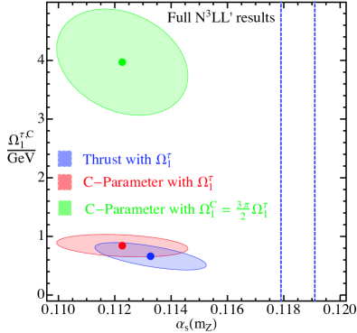
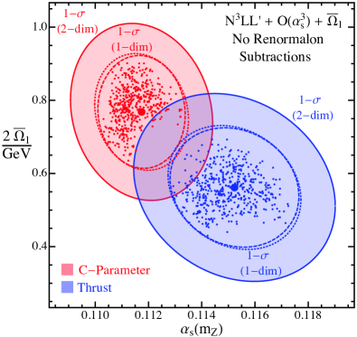
When testing for the universality of between thrust and C-parameter, there is an important calculable numerical factor of between and that must be accounted for; see Eq. (3). If we instead make a direct comparison of and , as shown in Fig. 13 (lowest blue ellipse vs uppermost green ellipse, respectively) then the results are - away from each other. Accounting for the factor to convert from to the upper green ellipse becomes the centermost red ellipse, and the thrust and C-parameter determinations agree with one another within uncertainties. Due to our high-precision control of perturbative effects, the parameters have only uncertainty, yielding a test of this universality at a higher level of precision than what has been previously achieved.
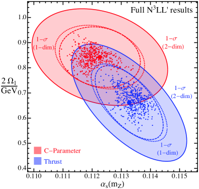
A zoomed-in version of this universality plot is shown in Fig. 14. The upper red ellipse again shows the result from fits to the C-parameter distribution, while the lower blue ellipse shows the result from thrust tail fits. For both we show the theory uncertainty (dashed lines) and combined theoretical and experimental (dotted lines) 39% CL uncertainty ellipses, as well as the solid ellipses which correspond to which is the standard 1- uncertainty for a two-parameter fit (68% CL). We see that the two analyses are completely compatible at the 1- level. An important ingredient to improve the overlap is the fact that we define the power corrections in the renormalon-free Rgap scheme. This is shown by contrasting the Rgap result in Fig. 14 with the overlap obtained when using the scheme for , as shown in Fig. 15.
VIII Conclusions and Comparison to Other Determinations
In this paper an accurate determination of from fits to the C-parameter distribution in the resummation region was presented. We fit to the tail of the distribution defined by , where the dominant hadronization effects are encoded in the first moment of the shape function , which is a power correction to the cross section. By fitting to data at multiple ’s, the strong coupling and can be simultaneously determined. The key points to our precise theoretical prediction are: a) higher-order resummation accuracy (N3LL′), achieved through an SCET factorization theorem, b) matrix elements and fixed-order kinematic power corrections, c) field-theoretical treatment of nonperturbative power corrections, and d) switching to a short-distance Rgap scheme, in which the sensitivity to infrared physics is reduced.
As our final result from the C-parameter global fit we obtain,
| (48) | ||||
where is defined in the scheme, and in the Rgap scheme (without hadron-mass effects) at the reference scales GeV. Here the respective total - uncertainties are shown. The results with individual - uncertainties quoted separately for the different sources of uncertainties are given in Eq. (45). Neglecting the nonperturbative effects incorporated by , the fit yields which exceeds the result in Eq. (48) by . This is consistent with a simple scaling argument one can derive from experimental data, presented in Ref. Hoang et al. (2014). We have also presented an updated thrust result, using our improved profiles for thrust and including bottom-mass and QED effects (but neglecting hadron-mass effects). This global fit for thrust gives
| (49) | ||||
Our theoretical prediction is the most complete treatment of C-parameter at this time, and, to the best of our knowledge, all sources of uncertainties have been included in our final uncertainty. Possible improvements which are expected to be negligible relative to our final uncertainty include finite bottom-mass effects, QED effects, and axial-singlet contributions. From our results there are a number of theoretical avenues that lead to small effects but which would be interesting to investigate further in the future. These are common to almost every event-shape analysis in the literature and include (i) resummation of logarithms for the nonsingular partonic cross section; (ii) the structure of nonperturbative power corrections for the nonsingular contributions (the last two points can be clarified with subleading SCET factorization theorems); (iii) analytic perturbative computations of the nonlogarithmic coefficients in the partonic soft function and the jet function, as well as the four-loop QCD cusp anomalous dimension (and to a lesser extent, the numerically determined constant of the two-loop partonic soft function); (iv) a better understanding of hadron-mass effects, and in particular their resummation beyond NLL; (v) a better theoretical description of the region around and above the shoulder. Concerning (i), and following the common lore, we have incorporated in our analysis the nonsingular contributions in fixed-order perturbation theory. However we have estimated the uncertainty related to the higher-order logarithms through the usual renormalization scale variation. Concerning (ii) we observe that the effect of these neglected power corrections is much smaller than naively expected, as can be seen from a comparison of our theoretical prediction and LEP data in the far-tail region. A first step towards clarifying (i) and (ii) has been taken in Refs. Freedman (2013); Freedman and Goerke (2014), for the case of thrust. The computation of missing perturbative terms (iii) is a priori feasible with current computational knowledge but they do not dominate our perturbative uncertainties. Concerning (iv) we have shown that hadron-mass effects have a very small impact on the determination of , and hence unless the rest of the sources of uncertainty become substantially smaller, our lack of knowledge does not constitute a problem. As for (v), our fits do not include data above the shoulder, so this problem has no impact on our fit. Nevertheless an analysis of these subleading effects would be interesting.
The same theoretical program carried out for thrust and C-parameter can be applied to other event-shapes, and the most prominent one is Heavy-Jet-Mass. This has partially worked out already in Ref. Chien and Schwartz (2010) at the purely perturbative level using fully canonical profiles. Their determination of is discussed below. For recoil-sensitive observables such as Jet Broadening Catani et al. (1992); Dokshitzer et al. (1998); Chiu et al. (2012a); Becher et al. (2011); Chiu et al. (2012b), one needs to deal with rapidity singularities, which imply that additional logs need to be resummed, and more complicated nonperturbative power corrections. The former has been pushed to the N2LL order in Ref. Becher and Bell (2012), and the latter has been studied in Ref. Becher and Bell (2014). Recoil-insensitive versions of Broadening have also been derived Larkoski et al. (2014), but not yet studied experimentally. Finally, it is very straightforward to generalize our theoretical treatment to the case of oriented event shapes Mateu and Rodrigo (2013), in which one additionally measures the angle between the beam and the thrust axes.
At this point we compare our result for with other determinations from event shapes at . To the best of our knowledge, the only analyses which fit to the tail of the C-parameter distribution using three-loop input are Ref. Dissertori et al. (2008) (using purely fix-order perturbation theory) and Ref. Dissertori et al. (2009) (including NLL resummation). Both analyses use Monte Carlo (MC) event generators to estimate hadronization effects, and fit for different values, finding values and respectively for a fit to the GeV data. These larger values are consistent with our fits which neglect power corrections, and following Ref. Abbate et al. (2011) we can conclude from this that MCs does not provide a reasonable estimate of the power corrections when including the higher-order perturbative contributions. In Ref. Gehrmann et al. (2010a) two-parameter global fits to the first five moments of the C-parameter distribution were performed. Hadronization effects are included via the frozen coupling model, and the value obtained, , is fully consistent with our result in Eq. (48) at 1-.
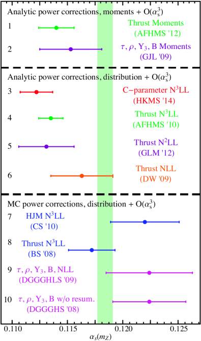
A graphical comparison with other event-shape determinations is shown in Fig. 16. The figure includes determinations where power corrections are estimated with MC generators, labeled by 7-10. Analyses 1-6 correspond to those in which power corrections were incorporated with an analytic method (either a shape function or the dispersive model). In the analyses 1-6 global fits are performed, whereas in the 7-10 analyses was determined at multiple values and the final result is an average of those. Only analyses 1 Abbate et al. (2012), 3 (this work), and 4 Abbate et al. (2011) used a completely field-theoretical approach for the power corrections. We also show both results from fits to the event-shape distributions (3-10) and from fits to moments of the event shape distribution (1 and 2). Although all analyses included matrix elements, different levels of resummation have been achieved. Analyses 2 Gehrmann et al. (2010a) and 10 Dissertori et al. (2008) did not included resummation; 6 Davison and Webber (2009) and 9 Dissertori et al. (2009) included NLL resummation; 5 Gehrmann et al. (2013) include N2LL resummation; and analyses 3,4,7, and 8 included N3LL resummation. Analyses 2, 9, and 10 simultaneously fit to many event shapes, whereas the others focused on a single observable: thrust (1, 4-6 and 8 Becher and Schwartz (2008)), Heavy-Jet-Mass (7 Chien and Schwartz (2010)), and C-parameter (3, which is this work). The analyses 1, 3, 4, 7 and 8 used SCET to perform Sudakov log resummation. All results that used an analytic treatment of power corrections have smaller values of . This is consistent with a simple dimensional analysis argument (see Refs. Abbate et al. (2011); Hoang et al. (2014)). Higher order resummation results in a convergent perturbation series and smaller uncertainties, and the Rgap scheme also reduces uncertainties. Accounting for the fact that results relying on MC for the treatment of power corrections should likely have larger hadronization uncertainties, all results are compatible among one another. The most precise results are however clearly in disagreement with the world average, which is dominated by lattice QCD results (see below) and shown as a translucent green band.
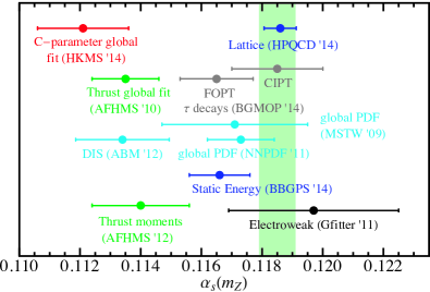
We conclude this work by comparing our result for with the results of a selection of recent analyses using other techniques and observables, as shown in Fig. 17. We include a N3LO analysis of data from deep inelastic scattering from the ABM group Alekhin et al. (2012), the global PDF fits of the MSTW group Martin et al. (2009) and the NNPDF collaboration Ball et al. (2012); the most recent (and accurate) determination from the HPQCD lattice collaboration Chakraborty et al. (2015), from the analysis of Wilson loops and pseudoscalar correlators; a determination analyzing the lattice prediction for the QCD static potential Bazavov et al. (2014); a reanalysis of electroweak precision observables by the Gfitter collaboration Flacher et al. (2009); the most recent analysis of tau decays in which the recently released ALEPH data was used together with the OPAL data; the previous determinations from fits to the thrust distribution Abbate et al. (2011) and moments of the thrust distribution Abbate et al. (2012); and of course the current world average Olive et al. (2014) (shown as the green band). The ABM (DIS) and thrust results are compatible with our determination, while in contrast the disagreement with either lattice QCD or the world average is -. Many other determinations lie between these two values. The source of this disagreement is an important open question.
Acknowledgements.
We thank the Erwin-Schrödinger Institute (ESI) for partial support in the framework of the ESI program “Jets and Quantum Fields for LHC and Future Colliders”. This work was supported by the offices of Nuclear and Particle Physics of the U.S. Department of Energy (DOE) under Contract DE-SC0011090, and the European Community’s Marie-Curie Research Networks under contract PITN-GA-2010-264564 (LHCphenOnet). IS was also supported in part by the Simons Foundation Investigator grant 327942. VM was supported by a Marie Curie Fellowship under contract PIOF-GA-2009-251174 while part of this work was completed. AH, VM, and IS are also supported in part by MISTI global seed funds. VM thanks H. Stenzel for explaining how to interpret the systematic uncertainties in the ALEPH dataset and Thomas Hahn for computer support.Appendix A Profile Formulae
In this appendix, we give the details for the profile functions that control the renormalization scales as laid out in Sec. II.2. For the soft profile function, we use the form,
| (50) |
where the physical meaning of the parameters is explained in Sec. II.2. The function (with ), which smoothly connects two straight lines of the form for and for is given by
| (53) | ||||
| (54) | ||||
For the jet scale, we use the form
| (55) |
which allows a slight modification of the natural relation between the scales in order to account for theoretical uncertainties.
For the subtraction scale, we have
| (56) |
As explained earlier, we take in the resummation region to avoid large logs and in the nonperturbative region to remove the renormalon. The function here interpolates smoothly between these two regions.
It is necessary to vary the profile parameters to estimate the theory uncertainty. We hold the difference between the parameters associated with the purely nonperturbative region constant: GeV, and we set as default values GeV, GeV. We are then left with nine profile parameters to vary during the theory scan, whose central values and variation ranges used in our analysis are: , , , , , , and . These variations are shown in Tab. 1.
Appendix B Comparison of thrust and C-parameter subtractions
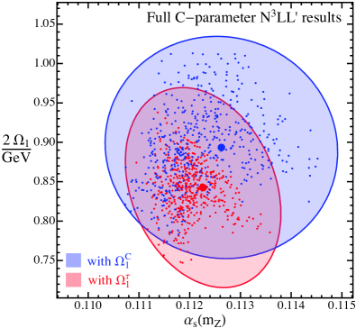
In Fig. 18 we compare fits performed in the Rgap scheme with C-parameter gap subtractions as the upper red ellipse, and for our default fits in the Rgap scheme with thrust gap subtractions as the lower blue ellipse. At N3LL′ order with C-parameter subtractions the results are and GeV, with . One can see that, even though both extractions are fully compatible, the thrust subtractions lead to smaller perturbative uncertainties. This is consistent with the better perturbative behavior observed for the cross section with thrust subtractions in Ref. Hoang et al. (2014).
Appendix C Comparison of thrust results with Ref. Abbate et al. (2011)
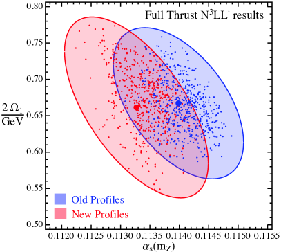
In Fig. 19 we compare global fits for the thrust distribution using the profiles of Ref. Abbate et al. (2011) (shown by the right ellipse in blue) and the profiles used here (shown by the left ellipse in red). As mentioned earlier, the profiles used here have several advantages over those of Ref. Abbate et al. (2011) in terms of their ability to independently impact the different regions of the thrust distribution, and in particular do a better job in the nonperturbative region (which is outside our fit region). The two versions of the profiles are consistent within their variations, and the fit results shown for 39% CL for two dimensions in Fig. 19 (which is 68% CL for each one-dimensional projection) are fully compatible.
References
- Kluth (2006) S. Kluth, Rept. Prog. Phys. 69, 1771 (2006), arXiv:hep-ex/0603011 .
- Bethke (2013) S. Bethke, Nucl.Phys.Proc.Suppl. 234, 229 (2013), arXiv:1210.0325 [hep-ex] .
- Gehrmann-De Ridder et al. (2007a) A. Gehrmann-De Ridder, T. Gehrmann, E. W. N. Glover, and G. Heinrich, Phys. Rev. Lett. 99, 132002 (2007a), arXiv:0707.1285 [hep-ph] .
- Davison and Webber (2009) R. A. Davison and B. R. Webber, Eur. Phys. J. C59, 13 (2009), arXiv:0809.3326 [hep-ph] .
- Becher and Schwartz (2008) T. Becher and M. D. Schwartz, JHEP 07, 034 (2008), arXiv:0803.0342 [hep-ph] .
- Dissertori et al. (2010) G. Dissertori, A. Gehrmann-De Ridder, T. Gehrmann, E. Glover, G. Heinrich, et al., Phys. Rev. Lett. 104, 072002 (2010), arXiv:0910.4283 [hep-ph] .
- Gehrmann-De Ridder et al. (2009) A. Gehrmann-De Ridder, T. Gehrmann, E. Glover, and G. Heinrich, JHEP 0905, 106 (2009), arXiv:0903.4658 [hep-ph] .
- Chien and Schwartz (2010) Y.-T. Chien and M. D. Schwartz, JHEP 08, 058 (2010), arXiv:1005.1644 [hep-ph] .
- Abbate et al. (2011) R. Abbate, M. Fickinger, A. H. Hoang, V. Mateu, and I. W. Stewart, Phys. Rev. D83, 074021 (2011), arXiv:1006.3080 .
- Abbate et al. (2012) R. Abbate, M. Fickinger, A. H. Hoang, V. Mateu, and I. W. Stewart, Phys. Rev. D86, 094002 (2012), arXiv:1204.5746 [hep-ph] .
- Gehrmann et al. (2013) T. Gehrmann, G. Luisoni, and P. F. Monni, Eur. Phys. J. C73, 2265 (2013), arXiv:1210.6945 [hep-ph] .
- Hoang et al. (2014) A. H. Hoang, D. W. Kolodrubetz, V. Mateu, and I. W. Stewart, (2014), arXiv:1411.6633 [hep-ph] .
- Farhi (1977) E. Farhi, Phys. Rev. Lett. 39, 1587 (1977).
- Parisi (1978) G. Parisi, Phys. Lett. B74, 65 (1978).
- Donoghue et al. (1979) J. F. Donoghue, F. Low, and S.-Y. Pi, Phys. Rev. D20, 2759 (1979).
- Bauer et al. (2001a) C. W. Bauer, S. Fleming, and M. E. Luke, Phys. Rev. D63, 014006 (2001a), hep-ph/0005275 .
- Bauer et al. (2001b) C. W. Bauer, S. Fleming, D. Pirjol, and I. W. Stewart, Phys. Rev. D 63, 114020 (2001b), hep-ph/0011336 .
- Bauer and Stewart (2001) C. W. Bauer and I. W. Stewart, Phys. Lett. B 516, 134 (2001), hep-ph/0107001 .
- Bauer et al. (2002a) C. W. Bauer, D. Pirjol, and I. W. Stewart, Phys. Rev. D65, 054022 (2002a), arXiv:hep-ph/0109045 .
- Bauer et al. (2002b) C. W. Bauer, S. Fleming, D. Pirjol, I. Z. Rothstein, and I. W. Stewart, Phys. Rev. D66, 014017 (2002b), hep-ph/0202088 .
- Catani and Webber (1997) S. Catani and B. Webber, JHEP 9710, 005 (1997), arXiv:hep-ph/9710333 [hep-ph] .
- Catani and Webber (1998) S. Catani and B. Webber, Phys. Lett. B427, 377 (1998), arXiv:hep-ph/9801350 [hep-ph] .
- Olive et al. (2014) K. Olive et al. (Particle Data Group), Chin. Phys. C38, 090001 (2014).
- Chakraborty et al. (2015) B. Chakraborty, C. Davies, B. Galloway, P. Knecht, J. Koponen, et al., Phys.Rev. D91, 054508 (2015), arXiv:1408.4169 [hep-lat] .
- Gehrmann et al. (2010a) T. Gehrmann, M. Jaquier, and G. Luisoni, Eur. Phys. J. C67, 57 (2010a), arXiv:0911.2422 [hep-ph] .
- Banfi et al. (2014) A. Banfi, H. McAslan, P. F. Monni, and G. Zanderighi, (2014), arXiv:1412.2126 [hep-ph] .
- Boito et al. (2015) D. Boito, M. Golterman, K. Maltman, J. Osborne, and S. Peris, Phys.Rev. D91, 034003 (2015), arXiv:1410.3528 [hep-ph] .
- Alekhin et al. (2012) S. Alekhin, J. Blumlein, and S. Moch, Phys. Rev. D86, 054009 (2012), arXiv:1202.2281 [hep-ph] .
- Bazavov et al. (2014) A. Bazavov, N. Brambilla, X. Garcia i Tormo, P. Petreczky, J. Soto, et al., Phys. Rev. D90, 074038 (2014), arXiv:1407.8437 [hep-ph] .
- Ball et al. (2012) R. D. Ball, V. Bertone, L. Del Debbio, S. Forte, A. Guffanti, et al., Phys.Lett. B707, 66 (2012), arXiv:1110.2483 [hep-ph] .
- Martin et al. (2009) A. D. Martin, W. J. Stirling, R. S. Thorne, and G. Watt, Eur. Phys. J. C64, 653 (2009), arXiv:0905.3531 [hep-ph] .
- Gehrmann-De Ridder et al. (2007b) A. Gehrmann-De Ridder, T. Gehrmann, E. W. N. Glover, and G. Heinrich, JHEP 12, 094 (2007b), arXiv:0711.4711 [hep-ph] .
- Gehrmann-De Ridder et al. (2014) A. Gehrmann-De Ridder, T. Gehrmann, E. Glover, and G. Heinrich, Comput. Phys. Commun. (2014), 10.1016/j.cpc.2014.07.024, arXiv:1402.4140 [hep-ph] .
- Weinzierl (2008) S. Weinzierl, Phys. Rev. Lett. 101, 162001 (2008), arXiv:0807.3241 [hep-ph] .
- Weinzierl (2009) S. Weinzierl, JHEP 06, 041 (2009), arXiv:0904.1077 [hep-ph] .
- Hoang and Stewart (2008) A. H. Hoang and I. W. Stewart, Phys. Lett. B660, 483 (2008), arXiv:0709.3519 [hep-ph] .
- Ligeti et al. (2008) Z. Ligeti, I. W. Stewart, and F. J. Tackmann, Phys. Rev. D78, 114014 (2008), arXiv:0807.1926 [hep-ph] .
- Gardi and Magnea (2003) E. Gardi and L. Magnea, JHEP 0308, 030 (2003), arXiv:hep-ph/0306094 [hep-ph] .
- Korchemsky and Tafat (2000) G. P. Korchemsky and S. Tafat, JHEP 10, 010 (2000), arXiv:hep-ph/0007005 .
- Dokshitzer and Webber (1995) Y. L. Dokshitzer and B. R. Webber, Phys. Lett. B352, 451 (1995), arXiv:hep-ph/9504219 .
- Lee and Sterman (2007) C. Lee and G. Sterman, Phys. Rev. D75, 014022 (2007), hep-ph/0611061 .
- Salam and Wicke (2001) G. P. Salam and D. Wicke, JHEP 05, 061 (2001), arXiv:hep-ph/0102343 .
- Mateu et al. (2013) V. Mateu, I. W. Stewart, and J. Thaler, Phys. Rev. D87, 014025 (2013), arXiv:1209.3781 [hep-ph] .
- Lunghi et al. (2003) E. Lunghi, D. Pirjol, and D. Wyler, Nucl. Phys. B649, 349 (2003), arXiv:hep-ph/0210091 .
- Bauer and Manohar (2004) C. W. Bauer and A. V. Manohar, Phys. Rev. D70, 034024 (2004), arXiv:hep-ph/0312109 .
- Becher and Neubert (2006) T. Becher and M. Neubert, Phys. Lett. B637, 251 (2006), arXiv:hep-ph/0603140 .
- Moch et al. (2004) S. Moch, J. A. M. Vermaseren, and A. Vogt, Nucl. Phys. B688, 101 (2004), arXiv:hep-ph/0403192 .
- Matsuura and van Neerven (1988) T. Matsuura and W. L. van Neerven, Z. Phys. C38, 623 (1988).
- Matsuura et al. (1989) T. Matsuura, S. C. van der Marck, and W. L. van Neerven, Nucl. Phys. B319, 570 (1989).
- Gehrmann et al. (2005) T. Gehrmann, T. Huber, and D. Maitre, Phys. Lett. B622, 295 (2005), arXiv:hep-ph/0507061 .
- Moch et al. (2005) S. Moch, J. A. M. Vermaseren, and A. Vogt, JHEP 08, 049 (2005), arXiv:hep-ph/0507039 .
- Lee et al. (2010) R. N. Lee, A. V. Smirnov, and V. A. Smirnov, JHEP 04, 020 (2010), arXiv:1001.2887 [hep-ph] .
- Baikov et al. (2009) P. A. Baikov, K. G. Chetyrkin, A. V. Smirnov, V. A. Smirnov, and M. Steinhauser, Phys. Rev. Lett. 102, 212002 (2009), arXiv:0902.3519 [hep-ph] .
- Gehrmann et al. (2010b) T. Gehrmann, E. Glover, T. Huber, N. Ikizlerli, and C. Studerus, JHEP 1006, 094 (2010b), arXiv:1004.3653 [hep-ph] .
- van Neerven (1986) W. L. van Neerven, Nucl. Phys. B268, 453 (1986).
- Ellis et al. (1980) R. K. Ellis, D. Ross, and A. Terrano, Phys. Rev. Lett. 45, 1226 (1980).
- Ellis et al. (1981) R. K. Ellis, D. A. Ross, and A. E. Terrano, Nucl. Phys. B178, 421 (1981).
- Catani and Seymour (1996) S. Catani and M. H. Seymour, Phys. Lett. B378, 287 (1996), arXiv:hep-ph/9602277 .
- Catani and Seymour (1997) S. Catani and M. H. Seymour, Nucl. Phys. B485, 291 (1997), arXiv:hep-ph/9605323 .
- Hoang and Kluth (2008) A. H. Hoang and S. Kluth, (2008), arXiv:0806.3852 [hep-ph] .
- Hoang et al. (2010) A. H. Hoang, A. Jain, I. Scimemi, and I. W. Stewart, Phys. Rev. D82, 011501 (2010), arXiv:0908.3189 [hep-ph] .
- Wolfram Research (2014) I. Wolfram Research, Mathematica Edition: Version 10.0 (Wolfram Research, Inc., Champaign, Illinois, 2014).
- gfo (2014) GFortran, Gnu compiler collection (gcc), Version 5.0.0 (Copyright (C) 2014 Free Software Foundation, Inc., 2014).
- Heister et al. (2004) A. Heister et al. (ALEPH), Eur. Phys. J. C35, 457 (2004).
- Abdallah et al. (2004) J. Abdallah et al. (DELPHI Collaboration), Eur.Phys.J. C37, 1 (2004), arXiv:hep-ex/0406011 [hep-ex] .
- Abreu et al. (1997) P. Abreu et al. (DELPHI), Z. Phys. C73, 229 (1997).
- Abreu et al. (1999) P. Abreu et al. (DELPHI), Phys. Lett. B456, 322 (1999).
- Wicke (1999) D. Wicke, (1999), wU-B-DIS-1999-05.
- Biebel et al. (1999) O. Biebel, P. Movilla Fernandez, and S. Bethke (JADE Collaboration), Phys. Lett. B459, 326 (1999), arXiv:hep-ex/9903009 [hep-ex] .
- Achard et al. (2004) P. Achard et al. (L3), Phys. Rept. 399, 71 (2004), arXiv:hep-ex/0406049 .
- Adeva et al. (1992) B. Adeva et al. (L3), Z. Phys. C55, 39 (1992).
- Abbiendi et al. (2005) G. Abbiendi et al. (OPAL), Eur. Phys. J. C40, 287 (2005), arXiv:hep-ex/0503051 .
- Abe et al. (1995) K. Abe et al. (SLD), Phys. Rev. D51, 962 (1995), arXiv:hep-ex/9501003 .
- Freedman (2013) S. M. Freedman, (2013), arXiv:1303.1558 [hep-ph] .
- Freedman and Goerke (2014) S. M. Freedman and R. Goerke, Phys. Rev. D90, 114010 (2014), arXiv:1408.6240 [hep-ph] .
- Catani et al. (1992) S. Catani, G. Turnock, and B. Webber, Phys. Lett. B295, 269 (1992).
- Dokshitzer et al. (1998) Y. L. Dokshitzer, A. Lucenti, G. Marchesini, and G. Salam, JHEP 9801, 011 (1998), arXiv:hep-ph/9801324 [hep-ph] .
- Chiu et al. (2012a) J.-y. Chiu, A. Jain, D. Neill, and I. Z. Rothstein, Phys. Rev. Lett. 108, 151601 (2012a), arXiv:1104.0881 [hep-ph] .
- Becher et al. (2011) T. Becher, G. Bell, and M. Neubert, Phys. Lett. B704, 276 (2011), arXiv:1104.4108 [hep-ph] .
- Chiu et al. (2012b) J.-Y. Chiu, A. Jain, D. Neill, and I. Z. Rothstein, JHEP 1205, 084 (2012b), arXiv:1202.0814 [hep-ph] .
- Becher and Bell (2012) T. Becher and G. Bell, JHEP 1211, 126 (2012), arXiv:1210.0580 [hep-ph] .
- Becher and Bell (2014) T. Becher and G. Bell, Phys. Rev. Lett. 112, 182002 (2014), arXiv:1312.5327 [hep-ph] .
- Larkoski et al. (2014) A. J. Larkoski, D. Neill, and J. Thaler, JHEP 1404, 017 (2014), arXiv:1401.2158 [hep-ph] .
- Mateu and Rodrigo (2013) V. Mateu and G. Rodrigo, JHEP 1311, 030 (2013), arXiv:1307.3513 .
- Dissertori et al. (2008) G. Dissertori et al., JHEP 02, 040 (2008), arXiv:0712.0327 [hep-ph] .
- Dissertori et al. (2009) G. Dissertori et al., JHEP 08, 036 (2009), arXiv:0906.3436 [hep-ph] .
- Flacher et al. (2009) H. Flacher et al., Eur. Phys. J. C60, 543 (2009), arXiv:0811.0009 [hep-ph] .