Spatial Interpolants

Abstract

We propose SplInter, a new technique for proving properties of heap-manipulating programs that marries (1) a new separation logic–based analysis for heap reasoning with (2) an interpolation-based technique for refining heap-shape invariants with data invariants. SplInter is property directed, precise, and produces counterexample traces when a property does not hold. Using the novel notion of spatial interpolants modulo theories, SplInter can infer complex invariants over general recursive predicates, e.g., of the form all elements in a linked list are even or a binary tree is sorted. Furthermore, we treat interpolation as a black box, which gives us the freedom to encode data manipulation in any suitable theory for a given program (e.g., bit vectors, arrays, or linear arithmetic), so that our technique immediately benefits from any future advances in SMT solving and interpolation.

1 Introduction

Since the problem of determining whether a program satisfies a given property is undecidable, every verification algorithm must make some compromise. There are two classical schools of program verification, which differ in the compromise they make: the static analysis school gives up refutation soundness (i.e., may report false positives); and the software model checking school gives up the guarantee of termination. In the world of integer program verification, both schools are well explored and enjoy cross-fertilization of ideas: each has its own strengths and uses in different contexts. In the world of heap-manipulating programs, the static analysis school is well-attended [35, 14, 12, 10], while the software model checking school has remained essentially vacant. This paper initiates a program to rectify this situation, by proposing one of the first path-based software model checking algorithms for proving combined shape-and-data properties.

The algorithm we propose, SplInter, marries two celebrated program verification ideas: McMillan’s lazy abstraction with interpolants (Impact) algorithm for software model checking [25], and separation logic, a program logic for reasoning about shape properties [32]. SplInter (like Impact) is based on a path-sampling methodology: given a program $P$ and safety property $\varphi$, SplInter constructs a proof that $P$ is memory safe and satisfies $\varphi$ by sampling a finite number of paths through the control-flow graph of $P$, proving them safe, and then assembling proofs for each sample path into a proof for the whole program. The key technical advance which enables SplInter is an algorithm for spatial interpolation, which is used to construct proofs in separation logic for the sample traces (serving the same function as Craig interpolation for first-order logic in Impact).

SplInter is able to prove properties requiring integrated heap and data (e.g., integer) reasoning by strengthening separation logic proofs with data refinements produced by classical Craig interpolation, using a technique we call spatial interpolation modulo theories. Data refinements are not tied to a specific logical theory, giving us a rather generic algorithm and freedom to choose an appropriate theory to encode a program’s data.

Fig. 1 summarizes the high-level operation of our algorithm. Given a program with no heap manipulation, SplInter only computes theory interpolants and behaves exactly like Impact, and thus one can thus view SplInter as a proper extension of Impact to heap manipulating programs. At the other extreme, given a program with no data manipulation, SplInter is a new shape analysis that uses path-based relaxation to construct memory safety proofs in separation logic.

There is a great deal of work in the static analysis school on shape analysis and on combined shape-and-data analysis, which we will discuss further in Sec. 8. We do not claim superiority over these techniques (which have had the benefit of 20 years of active development). SplInter, as the first member of the software model checking school, is not better; however, it is fundamentally different. Nonetheless, we will mention two of the features of SplInter (not enjoyed by any previous verification algorithm for shape-and-data properties) that make our approach worthy of exploration: path-based refinement and property-direction.

• Path-based refinement: This supports a progress guarantee by tightly correlating program exploration with refinement, and by avoiding imprecision due to lossy join and widening operations employed by abstract domains. SplInter does not report false positives, and produces counterexamples for violated properties. This comes, as usual, at the price of potential divergence.

• Property-direction: Rather than seeking the strongest invariant possible, we compute one that is just strong enough to prove that a desired property holds. Property direction enables scalable reasoning in rich program logics like the one described in this paper, which combines separation logic with first-order data refinements.

We have implemented an instantiation of our generic technique in the T2 verification tool [37], and used it to prove correctness of a number of programs, partly drawn from open source software, requiring combined data and heap invariants. Our results indicate the usability and promise of our approach.

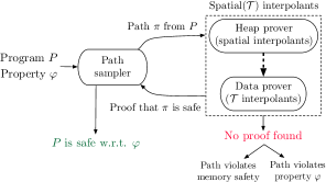
Figure 1: Overview of SplInter verification algorithm.

Contributions

We summarize our contributions as follows:

1. A generic property-directed algorithm for verifying and falsifying safety of programs with heap and data manipulation.

2. A precise and expressive separation logic analysis for computing memory safety proofs of program paths using a novel technique we term spatial interpolation.

3. A novel interpolation-based technique for strengthening separation logic proofs with data refinements.

4. An implementation and an evaluation of our technique for a fragment of separation logic with linked lists enriched with linear arithmetic refinements.

2 Overview

In this section, we demonstrate the operation of SplInter (Fig. 1) on the simple linked list example shown in Fig. 2. We assume that integers are unbounded (i.e., integer values are drawn from $\mathbb{Z}$ rather than machine integers) and

⬇

1: int i = nondet();

node* x = null;

2: while (i != 0)

node* tmp = malloc(node);

tmp->N = x;

tmp->D = i;

x = tmp;

i--;

3: while (x != null)

4: assert(x->D >= 0);

x = x->N;

Figure 2: Illustrative Example

that there is a struct called node denoting a linked list node, with a next pointer N and an integer (data) element D. The function nondet() returns a nondeterministic integer value. This program starts by building a linked list in the loop on location 2. The loop terminates if the initial value of i is $\geqslant 0$, in which case a linked list of size i is constructed, where data elements D of list nodes range from 1 to i. Then, the loop at location 3 iterates through the linked list asserting that the data element of each node in the list is $\geqslant 0$. Our goal is to prove that the assertion at location 4 is never violated.

Sample a Program Path

To start, we need a path $\pi$ through the program to the assertion at location 4. Suppose we start by sampling the path 1,2,2,3,4, that is, the path that goes through the first loop once, and enters the second loop arriving at the assertion. This path is illustrated in Fig. 3 (where 2a indicates the second occurrence of location 2). Our goal is to construct a Hoare-style proof of this path: an annotation of each location along the path with a formula describing reachable states, such that location 4 is annotated with a formula implying that x->D >= 0. This goal is accomplished in two phases. First, we use spatial interpolation to compute a memory safety proof for the path $\pi$ (Fig. 3(b)). Second, we use theory refinement to strengthen the memory safety proof and establish that the path satisfies the post-condition x->D >= 0 (Fig. 3(c)).

Compute Spatial Interpolants

The first step in constructing the proof is to find spatial interpolants: a sequence of separation logic formulas approximating the shape of the heap at each program location, and forming a Hoare-style memory safety proof of the path. Our spatial interpolation procedure is a two step process that first symbolically executes the path in a forward pass and then derives a weaker proof using a backward pass. The backward pass can be thought of as an under-approximate weakest precondition computation, which uses the symbolic heap from the forward pass to guide the under-approximation.

We start by showing the symbolic heaps in Fig. 3(a), which are the result of the forward pass obtained by symbolically executing only heap statements along this program path (i.e., the strongest postcondition along the path). The separation logic annotations in Fig. 3 follow standard notation (e.g., [14]), where a formula is of the form $\Pi:\Sigma$, where $\Pi$ is a Boolean first-order formula over heap variables (pointers) as well as data variables (e.g., $x=\textsf{null}$ or $i>0$), and $\Sigma$ is a spatial conjunction of heaplets (e.g., emp, denoting the empty heap, or $Z(x,y)$, a recursive predicate, e.g., that denotes a linked list between $x$ and $y$). For the purposes of this example, we assume a recursive predicate $\textsf{ls}(x,y)$ that describes linked lists. In our example, the symbolic heap at location 2a is $true:x\mapsto[d^{\prime},\textsf{null}],$ where the heap consists of a node, pointed to by variable $x$, with null in the N field and the (implicitly existentially quantified) variable $d^{\prime}$ in the D field (since so far we are only interested in heap shape and not data).

The symbolic heaps determine a memory safety proof of the path, but it is too strong and would likely not generalize to other paths. The goal of spatial interpolation is to find a sequence of annotations that are weaker than the symbolic heaps, but that still prove memory safety of the path. A sequence of spatial interpolants is shown in Fig. 3(b). Note that all spatial interpolants are implicitly spatially conjoined with true; for clarity, we avoid explicitly conjoining formulas with true in the figure. For example, location 2 is annotated with $true:\textsf{ls}(x,\textsf{null})*\textsf{true}$, indicating that there is a list on the heap, as well as other potential objects not required to show memory safety. We compute spatial interpolants by going backwards along the path and asking questions of the form: how much can we weaken the symbolic heap while still maintaining memory safety? We will describe how to answer such questions in Section 4.

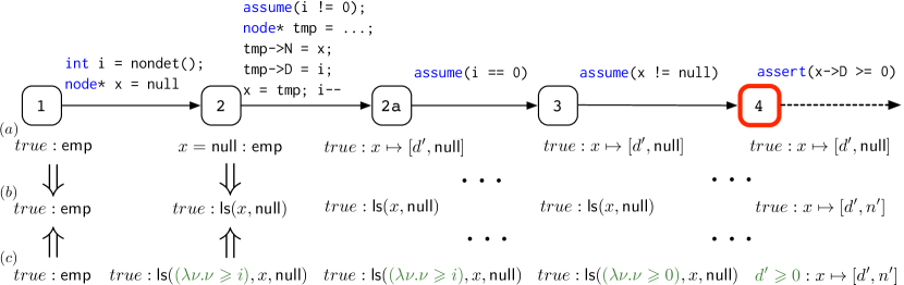
Figure 3: Path through program in Fig. 2, annotated with (a) results of forward symbolic execution, (b) spatial interpolants, and (c) spatial($\mathcal{T}$) interpolants, where $\mathcal{T}$ is linear integer arithmetic. Arrows $\Rightarrow$ indicate implication (entailment) direction.

Refine with Theory Interpolants

Spatial interpolants give us a memory safety proof as an approximate heap shape at each location. Our goal now is to strengthen these heap shapes with data refinements, in order to prove that the assertion at the end of the path is not violated. To do so, we generate a system of Horn clause constraints from the path in some first-order theory admitting interpolation (e.g., linear arithmetic). These Horn clauses carefully encode the path’s data manipulation along with the spatial interpolants, which tell us heap shape at each location along the path. A solution of this constraint system, which can be solved using off-the-shelf interpolant generation techniques (e.g., [26, 34]), is a refinement (strengthening) of the memory safety proof.

In this example, we encode program operations over integers in the theory of linear integer arithmetic, and use Craig interpolants to solve the system of constraints. A solution of this system is a set of linear arithmetic formulas that refine our spatial interpolants and, as a result, imply the assertion we want to prove holds. One possible solution is shown in Fig. 3(c). For example, location 2a is now labeled with $true\color[rgb]{0,0,0}:\mathsf{ls}(\color[rgb]{0,0.6,0}(\lambda\nu.\nu\geqslant i)\color[rgb]{0,0,0},x,\mathsf{null}),$ where the green parts of the formula are those added by refinement. Specifically, after refinement, we know that all elements in the list from $x$ to null after the first loop have data values greater than or equal to $i$, as indicated by the predicate $\color[rgb]{0,0.6,0}(\lambda\nu.\nu\geqslant i)$. (In Section 3, we formalize recursive predicates with data refinements.)

Location 4 is now annotated with $\color[rgb]{0,0.6,0}d^{\prime}\geqslant 0\color[rgb]{0,0,0}:x\mapsto[d^{\prime},n^{\prime}]*\textsf{true}$, which implies that x->D >= 0, thus proving that the path satisfies the assertion.

From Proofs of Paths to Proofs of Programs

We go from proofs of paths to whole program proofs implicitly by building an abstract reachability tree as in Impact [25]. To give a flavour for how this works, consider that the assertions at 2 and 2a are identical: this implies that this assertion is an inductive invariant at line 2. Since this assertion also happens to be strong enough to prove safety of the program, we need not sample any longer unrollings of the first loop. However, since we have not established the inductiveness of the assertion at 3, the proof is not yet complete and more traces need to be explored (in fact, exploring one more trace will do: consider the trace that unrolls the second loop once and shows that the second time 3 is visited can also be labeled with $\color[rgb]{0,0,0}true\color[rgb]{0,0,0}:\mathsf{ls}(\color[rgb]{0,0.6,0}(\lambda\nu.\nu\geqslant 0)\color[rgb]{0,0,0},x,\mathsf{null})$).

Since our high-level algorithm is virtually the same as Impact [25], we will not describe it further in the paper. For the remainder of this paper, we will concentrate on the novel contribution of our algorithm: computing spatial interpolants with theory refinements for program paths.

3 Preliminaries

3.1 Separation Logic

We define RSep, a fragment of separation logic formulas featuring points-to predicates and general recursive predicates refined by theory propositions.

$\begin{array}[]{lll||lrl}x,y\in\textsf{HVar}&\hskip 10.0pt\text{(Heap variables)}&&&E,F\in\textsf{HTerm}&::=\textsf{null}\mid x\\ a,b\in\textsf{DVar}&\hskip 10.0pt\text{(Data variables)}&&&\AE&::=A\ \mid E\\ A\in\textsf{DTerm}&\hskip 10.0pt\text{(Data terms)}&&&\Pi\in\textsf{Pure}&::=\emph{true}\mid E=E\mid E\neq E\mid\\ \varphi\in\textsf{DFormula}&\hskip 10.0pt\text{(Data formulas)}&&&&~{}~{}~{}~{}~{}\varphi\ \mid\Pi\land\Pi\\ Z\in\textsf{RPred}&\hskip 10.0pt\text{(Rec. predicates)}&&&H\in\textsf{Heaplet}&::=\textsf{true}\mid\textsf{emp}\mid E\mapsto[\vec{A},\vec{E}]\mid Z(\vec{\theta},\vec{E})\\ \theta\in\textsf{Refinement}&::=\lambda\vec{a}.\varphi&&&\Sigma\in\textsf{Spatial}&::=H\mid H*\Sigma\\ X\subseteq\textsf{Var}&::=x\mid a&&&P\in\textsf{RSep}&::=(\exists X.\;\Pi:\Sigma)\end{array}$

Figure 4: Syntax of RSep formulas.

Fig. 4 defines the syntax of RSep formulas. In comparison with the standard list fragment used in separation logic analyses (e.g., [3, 13, 27]), the differentiating features of RSep are: (1) General recursive predicates, for describing unbounded pointer structures like lists, trees, etc. (2) Recursive predicates are augmented with a vector of refinements, which are used to constrain the data values appearing on the data structure defined by the predicate, detailed below. (3) Each heap cell (points-to predicate), $E\mapsto[\vec{A},\vec{E}]$, is a record consisting of data fields (a vector $\vec{A}$ of DTerm) followed by heap fields (a vector $\vec{E}$ of HTerm). (Notationally, we will use $d_{i}$ to refer to the $i$th element of the vector $\vec{d}$, and $\vec{d}[t/d_{i}]$ to refer to the vector $\vec{d}$ with the $i$th element modified to $t$.) (4) Pure formulas contain heap and first-order data constraints.

Our definition is (implicitly) parameterized by a first-order theory $\mathcal{T}$. DVar denotes the set of theory variables, which we assume to be disjoint from HVar (the set of heap variables). DTerm and DFormula denote the sets of theory terms and formulas, and we assume that heap variables do not appear in theory terms.

For an RSep formula $P$, $\textsf{Var}(P)$ denotes its free (data and heap) variables. We treat a Spatial formula $\Sigma$ as a multiset of heaplets, and consider formulas to be equal when they are equal as multisets. For RSep formulas $P=(\exists X_{P}.\;\Pi_{P}:\Sigma_{P})$ and $Q=(\exists X_{Q}.\;\Pi_{Q}:\Sigma_{Q})$, we write $P*Q$ to denote the RSep formula

$$P*Q=(\exists X_{P}\cup X_{Q}.\;\Pi_{P}\land\Pi_{Q}:\Sigma_{P}*\Sigma_{Q})$$

assuming that $X_{P}$ is disjoint from $\textsf{Var}(Q)$ and $X_{Q}$ is disjoint from $\textsf{Var}(P)$ (if not, then $X_{P}$ and $X_{Q}$ are first suitably renamed). For a set of variables $X$, we write $(\exists X.\;P)$ to denote the RSep formula

$$(\exists X.\;P)=(\exists X\cup X_{P}.\;\Pi_{P}:\Sigma_{P})$$

Recursive predicates

Each recursive predicate $Z\in\textsf{RPred}$ is associated with a definition that describes how the predicate is unfolded. Before we formalize these definitions, we will give some examples.

The definition of the list segment predicate from Sec. 2 is:

$$\begin{split}\textsf{ls}(R,x,y)\equiv{}&(x=y:\textsf{emp})\lor{}\\ &(\exists d,n^{\prime}.\;x\neq y\land R(d):x\mapsto[d,n^{\prime}]*\textsf{ls}(R,n^{\prime},y))\end{split}$$

In the above, $R$ is a refinement variable, which may be instantiated to a concrete refinement $\theta\in\textsf{Refinement}$. For example, $\textsf{ls}((\lambda a.a\geqslant 0),x,y)$ indicates that there is a list from $x$ to $y$ where every element of the list is at least $0$.

A refined binary tree predicate is a more complicated example:

$$\textsf{bt}(Q,L,R,x)= \;(x=\textsf{null}:\textsf{emp})$$

$$\lor \;(\exists d,l,r.\;Q(d):x\mapsto[d,l,r]$$

$$\hskip 14.22636pt*\textsf{bt}((\lambda a.Q(a)\land L(d,a)),L,R,l)$$

$$\hskip 14.22636pt*\textsf{bt}((\lambda a.Q(a)\land R(d,a)),L,R,r))$$

This predicate has three refinement variables: a unary refinement $Q$ (which must be satisfied by every node in the tree), a binary refinement $L$ (which is a relation that must hold between every node and its descendants to the left), and a binary refinement $R$ (which is a relation that must hold between every node and its descendants to the right). For example,

$$\textsf{bt}((\lambda a.\emph{true}),(\lambda a,b.a\geqslant b),(\lambda a,b.a\leqslant b),x)$$

indicates that $x$ is the root of a binary search tree, and

$$\textsf{bt}((\lambda a.a\geqslant 0),(\lambda a,b.a\leqslant b),(\lambda a,b.a\leqslant b),x)$$

indicates that $x$ is the root of a binary min-heap with non-negative elements.

To formalize these definitions, we first define refinement terms and refined formulas: a refinement term $\tau$ is either (1) a refinement variable $R$ or (2) an abstraction $(\lambda a_{1},\dotsc,a_{n}.\Phi)$, where $\Phi$ is a refined formula. A refined formula is a conjunction where each conjunct is either a data formula (DFormula) or the application $\tau(\vec{A})$ of a refinement term to a vector of data terms (DTerm).

A predicate definition has the form

$$Z(\vec{R},\vec{x})\equiv(\exists X_{1}.\;\Pi_{1}\land\Phi_{1}:\Sigma_{1})\lor\dotsb\lor(\exists X_{n}.\;\Pi_{n}\land\Phi_{n}:\Sigma_{n})$$

where $\vec{R}$ is a vector of refinement variables, $\vec{x}$ is a vector of heap variables, and where refinement terms may appear as refinements in the spatial formulas $\Sigma_{i}$. We refer to the disjuncts of the above formula as the cases for $Z$, and define $\mathit{cases}(Z(\vec{R},\vec{x}))$ to be the set of cases of $Z$. $\vec{R}$ and $\vec{x}$ are bound in $\mathit{cases}(Z(\vec{R},\vec{x}))$, and we will assume that predicate definitions are closed, that is, for each case of $Z$, the free refinement variables belong to $\vec{R}$, the free heap variables belong to $\vec{x}$, and there are no free data variables. We also assume that they are well-typed in the sense that each refinement term $\tau$ is associated with an arity, and whenever $\tau(\vec{A})$ appears in a definition, the length of $\vec{A}$ is the arity of $\tau$.

Semantics

The semantics of our logic, defined by a satisfaction relation $s,h\models Q$, is essentially standard. Each predicate $Z\in\textsf{RPred}$ is defined to be the least solution to the following equivalence:

$$s,h\models Z(\vec{\theta},\vec{E})\iff\exists P\in\mathit{cases}(Z(\vec{R},\vec{x})).\ s,h\models P[\vec{\theta}/\vec{R},\vec{E}/\vec{x}]$$

Note that when substituting a $\lambda$-abstraction for a refinement variable, we implicitly $\beta$-reduce resulting applications. For example, $R(b)[(\lambda a.a\geqslant 0)/R]=b\geqslant 0$.

Semantic entailment is denoted by $P\models Q$, and provable entailment by $P\vdash Q$. When referring to a proof that $P\vdash Q$, we will mean a sequent calculus proof.

3.2 Programs

A program $\mathcal{P}$ is a tuple $\langle V,E,v_{\rm i},v_{\rm e}\rangle$, where

• $V$ is a set of control locations, with a distinguished entry node $v_{\rm i}\in V$ and error (exit) node $v_{\rm e}\in V$, and

• $E\subseteq V\times V$ is a set of directed edges, where each $e\in E$ is associated with a program command $e^{\rm c}$.

We impose the restriction that all nodes $V\setminus\{v_{\rm i}\}$ are reachable from $v_{\rm i}$ via $E$, and all nodes can reach $v_{\rm e}$. The syntax for program commands appears below. Note that the allocation command creates a record with $n$ data fields, $D_{1},\ldots,D_{n}$, and $m$ heap fields, $N_{1},\ldots,N_{m}$. To access the $i$th data field of a record pointed to by x, we use x->D_i (and similarly for heap fields). We assume that programs are well-typed, but not necessarily memory safe.  
 
Assignment: x := Æ
Heap store: x->N_i := E
Heap load: y := x->N_i Assumption: assume($\Pi$)
Data store: x->D_i := A
Data load: y := x->D_i Allocation: x := new($n,m$)
Disposal: free(x)

As is standard, we compile assert commands to reachability of $v_{\rm e}$.

4 Spatial Interpolants

In this section, we first define the notion of spatial path interpolants, which serve as memory safety proofs of program paths. We then describe a technique for computing spatial path interpolants. This algorithm has two phases: the first is a (forwards) symbolic execution phase, which computes the strongest memory safety proof for a path; the second is a (backwards) interpolation phase, which weakens the proof so that it is more likely to generalize.

Spatial path interpolants are bounded from below by the strongest memory safety proof, and (implicitly) from above by the weakest memory safety proof. Prior to considering the generation of inductive invariants using spatial path interpolants, consider what could be done with only one of the bounds, in general, with either a path-based approach or an iterative fixed-point computation. Without the upper bound, an interpolant or invariant could be computed using a standard forward transformer and widening. But this suffers from the usual problem of potentially widening too aggressively to prove the remainder of the path, necessitating the design of analyses which widen conservatively at the price of computing unnecessarily strong proofs. The upper bound neatly captures the information that must be preserved for the future execution to be proved safe. On the other hand, without the lower bound, an interpolant or invariant could be computed using a backward transformer (and lower widening). But this suffers from the usual problem that backward transformers in shape analysis explode, due to issues such as not knowing the aliasing relationship in the pre-state. The lower bound neatly captures such information, heavily reducing the potential for explosion. These advantages come at the price of operating over full paths from entry to error. Compared to a forwards iterative analysis, operating over full paths has the advantage of having information about the execution’s past and future when weakening at each point along the path. A forwards iterative analysis, on the other hand, trades the information about the future for information about many past executions through the use of join or widening operations.

The development in this section is purely spatial: we do not make use of data variables or refinements in recursive predicates. Our algorithm is thus of independent interest, outside of its context in this paper. We use Sep to refer to the fragment of RSep in which the only data formula (appearing in pure assertions and in refinements) is true (this fragment is equivalent to classical separation logic). An RSep formula $P$, in particular including those in recursive predicate definitions, determines a Sep formula $\underline{P}$ obtained by replacing all refinements (both variables and $\lambda$-abstractions) with $(\lambda\vec{a}.\emph{true})$ and all DFormulas in the pure part of $P$ with true. Since recursive predicates, refinements, and DFormulas appear only positively, $\underline{P}$ is no stronger than any refinement of $P$. Since all refinements in Sep are trivial, we will omit them from the syntax (e.g., we will write $Z(\vec{E})$ rather than $Z((\lambda\vec{a}.\emph{true}),\vec{E})$).

4.1 Definition

$\textsf{exec}(\texttt{x := new($k,l$)},\ (\exists X.\;\Pi:\Sigma))=$ $(\exists X\cup\{x^{\prime},\vec{d},\vec{n}\}.\;(\Pi:\Sigma)[x^{\prime}/x]*x\mapsto[\vec{d},\vec{n}])$
where $x^{\prime},\vec{d},\vec{n}$ are fresh, $\vec{d}=(d_{1},\ldots,d_{k})$, and $\vec{n}=(n_{1},\ldots,n_{l})$.

$\textsf{exec}(\texttt{free(x)},\ (\exists X.\;\Pi:\Sigma*z\mapsto[\vec{d},\vec{n}])=(\exists X.\;\Pi\land\Pi^{\neq}:\Sigma)$
where $\Pi:\Sigma*z\mapsto[\vec{d},\vec{n}]\vdash x=z$ and $\Pi^{\neq}$ is the
conjunction of all disequalities $x\neq y$ s.t $y\mapsto[\_,\_]\in\Sigma$.

$\textsf{exec}(\texttt{x := E},\ (\exists X.\;\Pi:\Sigma))=$ $(\exists X\cup\{x^{\prime}\}.\;(x=E[x^{\prime}/x])*(\Pi:\Sigma)[x^{\prime}/x])$
where $x^{\prime}$ is fresh.

$\textsf{exec}(\texttt{assume}(\Pi^{\prime}),\ (\exists X.\;\Pi:\Sigma))=(\exists X.\;\Pi\land\underline{\Pi^{\prime}}:\Sigma)$ .

$\textsf{exec}(\texttt{x->N${}_{i}$ := E},\ (\exists X.\;\Pi:\Sigma*z\mapsto[\vec{d},\vec{n}]))=$ $(\exists X.\;\Pi:\Sigma*x\mapsto[\vec{d},\vec{n}[E/n_{i}]])$
where $i\leqslant|\vec{n}|$ and $\Pi:\Sigma*z\mapsto[\vec{d},\vec{n}]\vdash x=z$ .

$\textsf{exec}(\texttt{y := x->N${}_{i}$},\ (\exists X.\;\Pi:\Sigma*z\mapsto[\vec{d},\vec{n}]))=$
$(\exists X\cup\{y^{\prime}\}.\;(y=n_{i}[y^{\prime}/y])*(\Pi:\Sigma*z\mapsto[\vec{d},\vec{n}])[y^{\prime}/y])$
where $i\leqslant|\vec{n}|$ and $\Pi:\Sigma*z\mapsto[\vec{d},\vec{n}]\vdash x=z$, and $y^{\prime}$ is fresh.

Figure 5: Symbolic execution for heap statements. Data statements are treated as skips.

We define a symbolic heap to be a Sep formula where the spatial part is a *-conjunction of points-to heaplets and the pure part is a conjunction of pointer (dis)equalities. Given a command c and a symbolic heap $S$, we use $\textsf{exec}(\texttt{c},S)$ to denote the symbolic heap that results from symbolically executing c starting in $S$ (the definition of exec is essentially standard [3], and is shown in Fig. 5).

Given a program path $\pi=e_{1},\ldots,e_{n}$, we obtain its strongest memory safety proof by symbolically executing $\pi$ starting from the empty heap emp. We call this sequence of symbolic heaps the symbolic execution sequence of $\pi$, and say that a path $\pi$ is memory-feasible if every formula in its symbolic execution sequence is consistent. The following proposition justifies calling this sequence the strongest memory safety proof.

Proposition 1

For a path $\pi$, if the symbolic execution sequence for $\pi$ is defined, then $\pi$ is memory safe. If $\pi$ is memory safe and memory-feasible, then its symbolic execution sequence is defined.

Recall that our strategy for proving program correctness is based on sampling and proving the correctness of several program paths (á la Impact [25]). The problem with strongest memory safety proofs is that they do not generalize well (i.e., do not generate inductive invariants).

One solution to this problem is to take advantage of property direction. Given a desired postcondition $P$ and a (memory-safe and -feasible) path $\pi$, the goal is to come up with a proof that is weaker than $\pi$’s symbolic execution sequence, but still strong enough to show that $P$ holds after executing $\pi$. Coming up with such “weak” proofs is how traditional path interpolation is used in Impact. In light of this, we define spatial path interpolants as follows:

Definition 1 (Spatial path interpolant)

Let $\pi=e_{1},\ldots,e_{n}$ be a program path with symbolic execution sequence $S_{0},\ldots,S_{n}$, and let $P$ be a Sep formula (such that $S_{n}\models P$). A spatial path interpolant for $\pi$ is a sequence $I_{0},\ldots,I_{n}$ of Sep formulas such that

• for each $i\in[0,n]$, $S_{i}\models I_{i}$;

• for each $i\in[1,n]$, $\{I_{i-1}\}\;e^{\rm c}_{i}\;\{I_{i}\}$ is a valid triple in separation logic; and

• $I_{n}\models P$ .

Our algorithm for computing spatial path interpolants is a backwards propagation algorithm that employs a spatial interpolation procedure at each backwards step. Spatial interpolants for a single command are defined as:

Definition 2 (Spatial interpolant)

Given Sep formulas $S$ and $I^{\prime}$ and a command c such that $\textsf{exec}(\texttt{c},S)\models I^{\prime}$, a spatial interpolant (for $S$, c, and $I^{\prime}$) is a Sep formula $I$ such that $S\models I$ and $\{I\}\;\texttt{c}\;\{I^{\prime}\}$ is valid.

Before describing the spatial interpolation algorithm, we briefly describe how spatial interpolation is used to compute path interpolants. Let us use $\textsf{itp}(S,\texttt{c},I)$ to denote a spatial interpolant for $S,\texttt{c},I$, as defined above. Let $\pi=e_{1},\ldots,e_{n}$ be a program path and let $P$ be a Sep formula. First, symbolically execute $\pi$ to compute a sequence $S_{0},\ldots,S_{n}$. Suppose that $S_{n}\vdash P$. Then we compute a sequence $I_{0},\ldots,I_{n}$ by taking $I_{n}=P$ and (for $k<n$) $I_{k}=\textsf{itp}(S_{k},e_{k+1}^{\rm c},I_{k+1})$. The sequence $I_{0},\ldots,I_{n}$ is clearly a spatial path interpolant.

4.2 Bounded Abduction

Our algorithm for spatial interpolation is based on an abduction procedure. Abduction refers to the inference of explanatory hypotheses from observations (in contrast to deduction, which derives conclusions from given hypotheses). The variant of abduction we employ in this paper, which we call bounded abduction, is simultaneously a form of abductive and deductive reasoning. Seen as a variant of abduction, bounded abduction adds a constraint that the abduced hypothesis be at least weak enough to be derivable from a given hypothesis. Seen as a variant of deduction, bounded abduction adds a constraint that the deduced conclusion be at least strong enough to imply some desired conclusion. Formally, we define bounded abduction as follows:

Definition 3 (Bounded abduction)

Let $L,M,R$ be Sep formulas, and let $X$ be a set of variables. A solution to the bounded abduction problem

$$L\vdash(\exists X.\;M*[\ ])\vdash R$$

is a Sep formula $A$ such that $L\models(\exists X.\;M*A)\models R$.

Note how, in contrast to bi-abduction [10] where a solution is a pair of formulas, one constrained from above and one from below, a solution to bounded abduction problems is a single formula that is simultaneously constrained from above and below. The fixed lower and upper bounds in our formulation of abduction give considerable guidance to solvers, in contrast to bi-abduction, where the bounds are part of the solution.

Sec. 6 presents our bounded abduction algorithm. For the remainder of this section, we will treat bounded abduction as a black box, and use $L\vdash(\exists X.\;M*[A])\vdash R$ to denote that $A$ is a solution to the bounded abduction problem.

4.3 Computing Spatial Interpolants

We now proceed to describe our algorithm for spatial interpolation. Given a command c and Sep formulas $S$ and $I^{\prime}$ such that $\textsf{exec}(\texttt{c},S)\vdash I^{\prime}$, this algorithm must compute a Sep formula $\textsf{itp}(S,\texttt{c},I^{\prime})$ that satisfies the conditions of Definition 2. Several examples illustrating this procedure are given in Fig. 3.

This algorithm is defined by cases based on the command c. We present the cases for the spatial commands; the corresponding data commands are similar.

Allocate

Suppose c is x := new($n,m$). We take $\textsf{itp}(S,\texttt{c},I^{\prime})=(\exists x.\;A)$, where $A$ is obtained as a solution to $\textsf{exec}(\texttt{c},S)\vdash(\exists\vec{a},\vec{z}.\;x\mapsto[\vec{a},\vec{z}]*[A])\vdash I^{\prime}$, and $\vec{a}$ and $\vec{z}$ are vectors of fresh variables of length $n$ and $m$, respectively.

Deallocate

Suppose c is free(x). We take $\textsf{itp}(S,\texttt{c},I^{\prime})=(\exists\vec{a},\vec{z}.\;I^{\prime}*x\mapsto[\vec{a},\vec{z}])$, where $\vec{a}$ and $\vec{z}$ are vectors of fresh variables whose lengths are determined by the unique heap cell which is allocated to $x$ in $S$.

Assignment

Suppose c is x := E. We take $\textsf{itp}(S,\texttt{c},I^{\prime})=I^{\prime}[E/x]$.

Store

Suppose c is x->N_i := E. We take $\textsf{itp}(S,\texttt{c},I^{\prime})=(\exists\vec{a},\vec{z}.\;A*x\mapsto[\vec{a},\vec{z}])$, where $A$ is obtained as a solution to $\textsf{exec}(\texttt{c},S)\vdash(\exists\vec{a},\vec{z}.\;x\mapsto[\vec{a},\vec{z}[E/z_{i}]]*[A])\vdash I^{\prime}$ and where $\vec{a}$ and $\vec{z}$ are vectors of fresh variables whose lengths are determined by the unique heap cell which is allocated to $x$ in $S$.

Example 1

Suppose that $S$ is $t\mapsto[4,y,\textsf{null}]*x\mapsto[2,\textsf{null},\textsf{null}]$ where the cells have one data and two pointer fields, c is t->N₀ := x, and $I^{\prime}$ is $\textsf{bt}(t)$. Then we can compute $\textsf{exec}(\texttt{c},S)=t\mapsto[4,x,\textsf{null}]*x\mapsto[2,\textsf{null},\textsf{null}]$, and then solve the bounded abduction problem

$$\textsf{exec}(\texttt{c},S)\vdash(\exists a,z_{1}.\;t\mapsto[a,x,z_{1}]*[\ ])\vdash I^{\prime}\ .$$

One possible solution is $A=\textsf{bt}(x)*\textsf{bt}(z_{1})$, which yields

$$\textsf{itp}(S,\texttt{c},I^{\prime})=(\exists a,z_{0},z_{1}.\;t\mapsto[a,z_{0},z_{1}]*\textsf{bt}(z_{1})*\textsf{bt}(x))\ .$$

Load

Suppose c is y := x->N_i. Suppose that $\vec{a}$ and $\vec{z}$ are vectors of fresh variables of lengths $|\vec{A}|$ and $|\vec{E}|$ where $S$ is of the form $\Pi:\Sigma*w\mapsto[\vec{A},\vec{E}]$ and $\Pi:\Sigma*w\mapsto[\vec{A},\vec{E}]\vdash x=w$ (this is the condition under which $\textsf{exec}(\texttt{c},S)$ is defined, see Fig. 5). Let $y^{\prime}$ be a fresh variable, and define $\overline{S}=(y=z_{i}[y^{\prime}/y])*(\Pi:\Sigma*w\mapsto[\vec{a},\vec{z}])[y^{\prime}/y]$. Note that $\overline{S}\vdash(\exists y^{\prime}.\;\overline{S})\equiv\textsf{exec}(\texttt{c},S)\vdash I^{\prime}$.

We take $\textsf{itp}(S,\texttt{c},I^{\prime})=(\exists\vec{a},\vec{z}.\;A[z_{i}/y,y/y^{\prime}]*x\mapsto[\vec{a},\vec{z}])$ where $A$ is obtained as a solution to $\overline{S}\vdash(\exists\vec{a},\vec{z}.\;x[y^{\prime}/y]\mapsto[\vec{a},\vec{z}]*[A])\vdash I^{\prime}$.

Example 2

Suppose that $S$ is $y=t:y\mapsto[1,\textsf{null},x]*x\mapsto[5,\textsf{null},\textsf{null}]$, c is y := y->N₁, and $I^{\prime}$ is $y\neq\textsf{null}:\textsf{bt}(t)$. Then $\overline{S}$ is

$$y=x\land y^{\prime}=t:y^{\prime}\mapsto[1,\textsf{null},x]*x\mapsto[5,\textsf{null},\textsf{null}]$$

We can then solve the bounded abduction problem

$$\overline{S}\vdash(\exists a,z_{0},z_{1}.\;y^{\prime}\mapsto[a,z_{0},z_{1}]*[\ ])\vdash I^{\prime}$$

A possible solution is $y\neq\textsf{null}\land y^{\prime}=t:\textsf{bt}(z_{0})*\textsf{bt}(z_{1})$, yielding
     $\textsf{itp}(S,\texttt{c},I^{\prime})=(\exists a,z_{0},z_{1}.z_{1}\neq\textsf{null}\land y=t:\textsf{bt}(z_{0})*\textsf{bt}(z_{1})*y\mapsto[a,z_{0},z_{1}])\ .$     $\lrcorner$

Assumptions

The interpolation rules defined up to this point cannot introduce recursive predicates, in the sense that if $I^{\prime}$ is a *-conjunction of points-to predicates then so is $\textsf{itp}(S,\texttt{c},I^{\prime})$. A *-conjunction of points-to predicates is exact in the sense that it gives the full layout of some part of the heap. The power of recursive predicates lies in their ability to be abstract rather than exact, and describe only the shape of the heap rather than its exact layout. It is a special circumstance that $\{P\}\;\texttt{{c}}\;\{I^{\prime}\}$ holds when $I^{\prime}$ is exact in this sense and $P$ is not: intuitively, it means that by executing c we somehow gain information about the program state, which is precisely the case for assume commands.

For an example of how spatial interpolation can introduce a recursive predicate at an assume command, consider the problem of computing an interpolant

$$\textsf{itp}(S,\texttt{assume(x $\neq\textsf{null}$)},(\exists a,z.\;x\mapsto[a,z]*\textsf{true}))$$

where $S\equiv x\mapsto[d,y]*y\mapsto[d^{\prime},\textsf{null}]$: a desirable interpolant may be $\textsf{ls}(x,\textsf{null})*\textsf{true}$. The disequality introduced by the assumption ensures that one of the $\mathit{cases}$ of the recursive predicate $\textsf{ls}(x,\textsf{null})$ (where the list from $x$ to null is empty) is impossible, which implies that the other case (where $x$ is allocated) must hold.

Towards this end, we now define an auxiliary function intro which we will use to introduce recursive predicates for the assume interpolation rules. Let $P,Q$ be Sep formulas such that $P\vdash Q$, let $Z$ be a recursive predicate and $\vec{E}$ be a vector of heap terms. We define $\textsf{intro}(Z,\vec{E},P,Q)$ as follows: if $P\vdash(\exists\emptyset.\;Z(\vec{E})*[A])\vdash Q$ has a solution and $A\nvdash Q$, define $\textsf{intro}(Z,\vec{E},P,Q)=Z(\vec{E})*A$. Otherwise, define $\textsf{intro}(Z,\vec{E},P,Q)=Q$.

Intuitively, the abduction problem has a solution when $P$ implies $Z(\vec{E})$ and $Z(\vec{E})$ can be excised from $Q$. The condition $A\nvdash Q$ is used to ensure that the excision from $Q$ is non-trivial (i.e., the part of the heap that satisfies $Z(\vec{E})$ “consumes” some heaplet of $Q$).

To define the interpolation rule for assumptions, suppose c is assume(E $\neq$ F) (the case of equality assumptions is similar). Letting $\{\langle Z_{i},\vec{E}_{i}\rangle\}_{i\leqslant n}$ be an enumeration of the (finitely many) possible choices of $Z$ and $\vec{E}$, we define a formula $M$ to be the result of applying intro to $I^{\prime}$ over all possible choices of $Z$ and $\vec{E}$:

$$M=\textsf{intro}(Z_{1},\vec{E}_{1},S\land E\neq F,\textsf{intro}(Z_{2},\vec{E}_{2},S\land E\neq F,\dotsc))$$

where the innermost occurrence of intro in this definition is $\textsf{intro}(Z_{n},\vec{E}_{n},S\land E\neq F,I^{\prime})$. Since intro preserves entailment (in the sense that if $P\vdash Q$ then $P\vdash\textsf{intro}(Z,\vec{E},P,Q)$), we have that $S\land E\neq F\vdash M$. From a proof of $S\land E\neq F\vdash M$, we can construct a formula $M^{\prime}$ which is entailed by $S$ and differs from $M$ only in that it renames variables and exposes additional equalities and disequalities implied by $S$, and take $\textsf{itp}(S,\texttt{c},I^{\prime})$ to be this $M^{\prime}$.

The construction of $M^{\prime}$ from $M$ is straightforward but tedious. The procedure is detailed in Appendix 0.D ; here, we will just give an example to give intuition on why it is necessary. Suppose that $S$ is $x=w:y\mapsto z$ and $I^{\prime}$ is $\textsf{ls}(w,z)$, and c is assume($x$ = $y$). Since there is no opportunity to introduce new recursive predicates in $I^{\prime}$, $M$ is simply $\textsf{ls}(w,z)$. However, $M$ is not a valid interpolant since $S\not\models M$, so we must expose the equality $x=w$ and rename $w$ to $y$ in the list segment in $M^{\prime}\equiv x=w:\textsf{ls}(y,z)$.

In practice, it is undesirable to enumerate all possible choices of $Z$ and $\vec{E}$ when constructing $M$ (considering that if there are $k$ in-scope data terms, a recursive predicate of arity $n$ requires enumerating $k^{n}$ choices for $\vec{E}$). A reasonable heuristic is to let $\Pi$ be the strongest pure formula implied by $S$, and enumerate only those combinations of $Z$ and $\vec{E}$ such that there is some $\Pi^{\prime}:\Sigma^{\prime}\in\mathit{cases}(Z(\vec{R},\vec{x}))$ such that $\underline{\Pi^{\prime}}[\vec{E}/\vec{x}]\land\Pi\land x\neq y$ is unsatisfiable. For example, for assume(x $\neq$ y), this heuristic means that we enumerate only $\langle x,y\rangle$ and $\langle y,x\rangle$ (i.e, we attempt to introduce a list segment from $x$ to $y$ and from $y$ to $x$).

We conclude this section with a theorem stating the correctness of our spatial interpolation procedure.

Theorem 4.1

Let $S$ and $I^{\prime}$ be Sep formulas and let c be a command such that $\textsf{exec}(\texttt{c},S)\vdash I^{\prime}$. Then $\textsf{itp}(S,\texttt{c},I^{\prime})$ is a spatial interpolant for $S$, c, and $I^{\prime}$.

5 Spatial Interpolation Modulo Theories

  Entailment rules  

Star $$\displaystyle{\hbox{\hskip 124.83215pt\vbox{\hbox{\hskip-124.83215pt\hbox{\hbox{$\displaystyle\displaystyle\mathcal{C}_{0}\ \blacktriangleright\ \Pi\land\Phi:\Sigma_{0}\vdash\Pi^{\prime}\land\Phi^{\prime}:\Sigma_{0}^{\prime}$}\hskip 18.00003pt\hbox{\hbox{$\displaystyle\displaystyle\mathcal{C}_{1}\ \blacktriangleright\ \Pi\land\Phi:\Sigma_{1}\vdash\Pi^{\prime}\land\Phi^{\prime}:\Sigma_{1}^{\prime}$}}}}\vbox{}}}\over\hbox{\hskip 79.19612pt\vbox{\vbox{}\hbox{\hskip-79.1961pt\hbox{\hbox{$\displaystyle\displaystyle\mathcal{C}_{0};\mathcal{C}_{1}\ \blacktriangleright\ \Pi\land\Phi:\Sigma_{0}*\Sigma_{1}\vdash\Pi^{\prime}\land\Phi^{\prime}:\Sigma_{0}^{\prime}*\Sigma_{1}^{\prime}$}}}}}} \displaystyle{\hbox{\hskip 13.31801pt\vbox{\hbox{\hskip-13.31801pt\hbox{\hbox{$\displaystyle\displaystyle\Pi\models\Pi^{\prime}$}}}\vbox{}}}\over\hbox{\hskip 91.31795pt\vbox{\vbox{}\hbox{\hskip-91.31795pt\hbox{\hbox{$\displaystyle\displaystyle\Phi^{\prime}\leftarrow\Phi\ \blacktriangleright\ \Pi\land\Phi:E\mapsto[\vec{A},\vec{F}]\vdash\Pi^{\prime}\land\Phi^{\prime}:E\mapsto[\vec{A},\vec{F}]$}}}}}} \displaystyle{\hbox{\hskip 66.7265pt\vbox{\hbox{\hskip-66.7265pt\hbox{\hbox{$\displaystyle\displaystyle\mathcal{C}\ \blacktriangleright\ \Pi:\Sigma\vdash\Pi^{\prime}:\Sigma^{\prime}*P[\vec{\tau}/\vec{R},\vec{E}/\vec{x}]$}}}\vbox{}}}\over\hbox{\hskip 57.81798pt\vbox{\vbox{}\hbox{\hskip-57.81798pt\hbox{\hbox{$\displaystyle\displaystyle\mathcal{C}\ \blacktriangleright\ \Pi:\Sigma\vdash\Pi^{\prime}:\Sigma^{\prime}*Z(\vec{\tau},\vec{E})$}}}}}} P\in\mathit{cases}(Z(\vec{R},\vec{x})) \displaystyle{\hbox{\hskip 129.24738pt\vbox{\hbox{\hskip-129.24738pt\hbox{\hbox{$\displaystyle\displaystyle\mathcal{C}_{1}\ \blacktriangleright\ \Pi:\Sigma*P_{1}[\vec{\tau}/\vec{R},\vec{E}/\vec{x}]\vdash\Pi^{\prime}:\Sigma^{\prime}$}\hskip 18.00003pt\hbox{\hbox{$\displaystyle\displaystyle\dotsi$}\hskip 18.00003pt\hbox{\hskip-72.00168pt\hbox{\hbox{$\displaystyle\displaystyle\mathcal{C}_{n}\ \blacktriangleright\ \Pi:\Sigma*P_{n}[\vec{\tau}/\vec{R},\vec{E}/\vec{x}]\vdash\Pi^{\prime}:\Sigma^{\prime}$}}}}}}\vbox{\hbox{\hskip-72.00168pt\hbox{\hbox{$\displaystyle\displaystyle\mathcal{C}_{n}\ \blacktriangleright\ \Pi:\Sigma*P_{n}[\vec{\tau}/\vec{R},\vec{E}/\vec{x}]\vdash\Pi^{\prime}:\Sigma^{\prime}$}}}\vbox{}}}}\over\hbox{\hskip 71.84058pt\vbox{\vbox{}\hbox{\hskip-71.84058pt\hbox{\hbox{$\displaystyle\displaystyle\mathcal{C}_{1};\dotsc{;}\,\mathcal{C}_{n}\ \blacktriangleright\ \Pi:\Sigma*Z(\vec{\tau},\vec{E})\vdash\Pi^{\prime}:\Sigma^{\prime}$}}}}}} \{P_{1},\dotsc,P_{n}\}= \mathit{cases}(Z(\vec{R},\vec{x})) \displaystyle{\hbox{\hskip 13.31801pt\vbox{\hbox{\hskip-13.31801pt\hbox{\hbox{$\displaystyle\displaystyle\Pi\models\Pi^{\prime}$}}}\vbox{}}}\over\hbox{\hskip 150.74358pt\vbox{\vbox{}\hbox{\hskip-150.74358pt\hbox{\hbox{\hbox{$\displaystyle\displaystyle\Phi^{\prime}\leftarrow\Phi;\Psi_{1}^{\prime}\leftarrow\Psi_{1}\land\Phi;\dotsc{;}\,\Psi_{|\vec{\tau}|}^{\prime}\leftarrow\Psi_{|\vec{\tau}|}\land\Phi\blacktriangleright$}}\hskip 18.00003pt\hbox{$\displaystyle\displaystyle\Pi\land\Phi:Z(\vec{\tau},\vec{E})\vdash\Pi^{\prime}\land\Phi^{\prime}:Z(\vec{\tau^{\prime}},\vec{E})$}}}}}} \tau_{i}=(\lambda\vec{a}_{i}.\Psi_{i}) \tau_{i}^{\prime}=(\lambda\vec{a}_{i}.\Psi_{i}^{\prime})$$        Points-to        Fold         Unfold          Predicate   Where and

  Execution rules  

Data-Assume $$\displaystyle{\hbox{\hskip 34.01534pt\vbox{\hbox{\hskip-34.01532pt\hbox{\hbox{$\displaystyle\displaystyle\mathcal{C}\ \blacktriangleright\ P\land\varphi\vdash Q$}}}\vbox{}}}\over\hbox{\hskip 53.81538pt\vbox{\vbox{}\hbox{\hskip-53.81537pt\hbox{\hbox{$\displaystyle\displaystyle\mathcal{C}\ \blacktriangleright\ \{P\}\;\texttt{assume($\displaystyle\varphi$)}\;\{Q\}$}}}}}} \displaystyle{\hbox{\hskip 60.74919pt\vbox{\hbox{\hskip-60.74919pt\hbox{\hbox{$\displaystyle\displaystyle\mathcal{C}\ \blacktriangleright\ P\vdash\Pi\land\Phi:\Sigma*x\mapsto[\vec{A},\vec{E}]$}}}\vbox{}}}\over\hbox{\hskip 61.40166pt\vbox{\vbox{}\hbox{\hskip-61.40166pt\hbox{\hbox{$\displaystyle\displaystyle\mathcal{C}\ \blacktriangleright\ \{P\}\;\texttt{free(x)}\;\{\Pi\land\Phi:\Sigma\}$}}}}}} \displaystyle{\hbox{\hskip 84.29749pt\vbox{\hbox{\hskip-84.29747pt\hbox{\hbox{$\displaystyle\displaystyle\mathcal{C}_{0}\ \blacktriangleright\ \{P\}\;\texttt{$\displaystyle\pi_{0}$}\;\{\widehat{O}\}$}\hskip 18.00003pt\hbox{\hbox{$\displaystyle\displaystyle\mathcal{C}_{1}\ \blacktriangleright\ \{\widehat{O}\}\;\texttt{$\displaystyle\pi_{1}$}\;\{Q\}$}}}}\vbox{}}}\over\hbox{\hskip 49.99185pt\vbox{\vbox{}\hbox{\hskip-49.99185pt\hbox{\hbox{$\displaystyle\displaystyle\mathcal{C}_{0};\mathcal{C}_{1}\ \blacktriangleright\ \{P\}\;\texttt{$\displaystyle\pi_{0};\pi_{1}$}\;\{Q\}$}}}}}} \displaystyle{\hbox{\hskip 151.36311pt\vbox{\hbox{\hskip-151.3631pt\hbox{\hbox{$\displaystyle\displaystyle\mathcal{C}_{0}\ \blacktriangleright\ P\vdash(\exists X.\;\Pi\land\widehat{\Phi}:\widehat{\Sigma}*x\mapsto[\vec{A},\vec{E}])$}\hskip 18.00003pt\hbox{\hskip-143.93417pt\hbox{\hbox{$\displaystyle\displaystyle\mathcal{C}_{1}\ \blacktriangleright\ (\exists X,a^{\prime}.\;\Pi[a^{\prime}/a]\land\widehat{\Phi}[a^{\prime}/a]\land a=A_{i}[a^{\prime}/a]\colon(\widehat{\Sigma}*x\mapsto[\vec{A},\vec{E}])[a^{\prime}/a])\vdash Q$}}}}}\vbox{\hbox{\hskip-143.93417pt\hbox{\hbox{$\displaystyle\displaystyle\mathcal{C}_{1}\ \blacktriangleright\ (\exists X,a^{\prime}.\;\Pi[a^{\prime}/a]\land\widehat{\Phi}[a^{\prime}/a]\land a=A_{i}[a^{\prime}/a]\colon(\widehat{\Sigma}*x\mapsto[\vec{A},\vec{E}])[a^{\prime}/a])\vdash Q$}}}\vbox{}}}}\over\hbox{\hskip 62.02232pt\vbox{\vbox{}\hbox{\hskip-62.02232pt\hbox{\hbox{$\displaystyle\displaystyle\mathcal{C}_{0};\mathcal{C}_{1}\ \blacktriangleright\ \{P\}\;\texttt{a := x->D${}_{i}$}\;\{Q\}$}}}}}} \displaystyle{\hbox{\hskip 104.60881pt\vbox{\hbox{\hskip-104.6088pt\hbox{\hbox{$\displaystyle\displaystyle\mathcal{C}\ \blacktriangleright\ (\exists a^{\prime}.\;\Pi\land\Phi[a^{\prime}/a]\land a=A[a^{\prime}/a]:\Sigma[a^{\prime}/a]\vdash Q)$}}}\vbox{}}}\over\hbox{\hskip 61.8076pt\vbox{\vbox{}\hbox{\hskip-61.80759pt\hbox{\hbox{$\displaystyle\displaystyle\mathcal{C}\ \blacktriangleright\ \{\Pi\land\Phi\colon\Sigma\}\;\texttt{a := A}\;\{Q\}$}}}}}} \displaystyle{\hbox{\hskip 131.78232pt\vbox{\hbox{\hskip-131.78232pt\hbox{\hbox{$\displaystyle\displaystyle\mathcal{C}_{0}\ \blacktriangleright\ P\vdash(\exists X.\;\Pi\land\widehat{\Phi}:\widehat{\Sigma}*x\mapsto[\vec{A},\vec{E}])$}\hskip 18.00003pt\hbox{\hskip-104.77258pt\hbox{\hbox{$\displaystyle\displaystyle\mathcal{C}_{1}\ \blacktriangleright\ (\exists X,a^{\prime}.\;\Pi\land\widehat{\Phi}\land a^{\prime}=A:\widehat{\Sigma}*x\mapsto[\vec{A}[a^{\prime}/A_{i}],\vec{E}])\vdash Q$}}}}}\vbox{\hbox{\hskip-104.77258pt\hbox{\hbox{$\displaystyle\displaystyle\mathcal{C}_{1}\ \blacktriangleright\ (\exists X,a^{\prime}.\;\Pi\land\widehat{\Phi}\land a^{\prime}=A:\widehat{\Sigma}*x\mapsto[\vec{A}[a^{\prime}/A_{i}],\vec{E}])\vdash Q$}}}\vbox{}}}}\over\hbox{\hskip 63.14732pt\vbox{\vbox{}\hbox{\hskip-63.14732pt\hbox{\hbox{$\displaystyle\displaystyle\mathcal{C}_{0};\mathcal{C}_{1}\ \blacktriangleright\ \{P\}\;\texttt{x->D${}_{i}$ := A}\;\{Q\}$}}}}}} \displaystyle{\hbox{\hskip 106.26921pt\vbox{\hbox{\hskip-106.2692pt\hbox{\hbox{$\displaystyle\displaystyle\mathcal{C}\ \blacktriangleright\ (\exists x^{\prime},\vec{a},\vec{x}.\;\Pi[x^{\prime}/x]\land\Phi:\Sigma[x^{\prime}/x]*x\mapsto[\vec{a},\vec{x}])\vdash Q$}}}\vbox{}}}\over\hbox{\hskip 77.70972pt\vbox{\vbox{}\hbox{\hskip-77.70972pt\hbox{\hbox{$\displaystyle\displaystyle\mathcal{C}\ \blacktriangleright\ \{\Pi\land\Phi\colon\Sigma\}\;\texttt{x := new($\displaystyle n$,$\displaystyle m$)}\;\{Q\}\vspace{-19pt}$}}}}}}$$        Free        Sequence        Data-Load        Data-Assign        Data-Store        Alloc

Figure 6: Constraint generation.

Refined memory safety proof $\zeta^{\prime}$
$\color[rgb]{0.35,0.35,0.35}\{R_{0}(i):\textsf{true}\}$
i = nondet(); x = null
$\color[rgb]{0.35,0.35,0.35}\{R_{1}(i):\textsf{ls}((\lambda a.R_{\textsf{ls}1}(\nu,i)),x,\textsf{null})*\textsf{true}\}$
assume(i != 0); …; i-​-;
$\color[rgb]{0.35,0.35,0.35}\{R_{2}(i):\textsf{ls}((\lambda a.R_{\textsf{ls}2}(\nu,i)),x,\textsf{null})*\textsf{true}\}$
assume(i == 0)
$\color[rgb]{0.35,0.35,0.35}\{R_{3}(i):\textsf{ls}((\lambda a.R_{\textsf{ls}3}(\nu,i)),x,\textsf{null})*\textsf{true}\}$
assume(x != null)
$\color[rgb]{0.35,0.35,0.35}\{(\exists d^{\prime},y.\;R_{4}(i,d^{\prime}):x\mapsto[d^{\prime},y]*\textsf{true})\}$

Constraint system $\mathcal{C}$
$R_{0}(i^{\prime})\leftarrow\textit{true}$
$R_{1}(i^{\prime})\leftarrow R_{0}(i)$
$R_{2}(i^{\prime})\leftarrow R_{1}(i)\land i\neq 0\land i^{\prime}=i+1$
$R_{3}(i)\leftarrow R_{2}(i)\land i=0$
$R_{4}(i,d^{\prime})\leftarrow R_{3}(i)\land R_{\textsf{ls}3}(d^{\prime},i)$
$R_{\textsf{ls}2}(\nu,i^{\prime})\leftarrow R_{1}(i)\land R_{\textsf{ls}1}(\nu,i)\land i\neq 0\land i^{\prime}=i+1$
$R_{\textsf{ls}2}(\nu,i^{\prime})\leftarrow R_{1}(i)\land\nu=i\land i\neq 0\land i^{\prime}=i+1$
$R_{\textsf{ls}3}(\nu,i)\leftarrow R_{2}(i)\land R_{\textsf{ls}2}(\nu,i)\land i=0$
$d^{\prime}\geqslant 0\leftarrow R_{4}(i,d^{\prime})$

Solution $\sigma$
$R_{0}(i):\textit{true}$
$R_{1}(i):\textit{true}$
$R_{2}(i):\textit{true}$
$R_{3}(i):\textit{true}$
$R_{4}(i,d^{\prime}):d^{\prime}\geqslant 0$
$R_{\textsf{ls}1}(\nu,i):\nu\geqslant i$
$R_{\textsf{ls}2}(\nu,i):\nu\geqslant i$
$R_{\textsf{ls}3}(\nu,i):\nu\geqslant 0$

Figure 7: Example constraints.

We now consider the problem of refining (or strengthening) a given separation logic proof of memory safety with information about (non-spatial) data. This refinement procedure results in a proof of a conclusion stronger than can be proved by reasoning about the heap alone. In view of our example from Fig. 3, this section addresses how to derive the third sequence (Spatial Interpolants Modulo Theories) from the second (Spatial Interpolants).

The input to our spatial interpolation modulo theories procedure is a path $\pi$, a separation logic (Sep) proof $\zeta$ of the triple $\{\textit{true}:\textsf{emp}\}\;\texttt{$\pi$}\;\{\textit{true}:\textsf{true}\}$ (i.e., a memory safety proof for $\pi$), and a postcondition $\varphi$. The goal is to transform $\zeta$ into an RSep proof of the triple $\{\textit{true}:\textsf{emp}\}\;\texttt{$\pi$}\;\{\varphi:\textsf{true}\}$. The high-level operation of our procedure is as follows. First, we traverse the memory safety proof $\zeta$ and build (1) a corresponding refined proof $\zeta^{\prime}$ where refinements may contain second-order variables, and (2) a constraint system $\mathcal{C}$ which encodes logical dependencies between the second-order variables. We then attempt to find a solution to $\mathcal{C}$, which is an assignment of data formulas to the second-order variables such that all constraints are satisfied. If we are successful, we use the solution to instantiate the second-order variables in $\zeta^{\prime}$, which yields a valid RSep proof of the triple $\{\textit{true}:\textsf{emp}\}\;\texttt{$\pi$}\;\{\varphi:\textsf{true}\}$.

Horn Clauses

The constraint system produced by our procedure is a recursion-free set of Horn clauses, which can be solved efficiently using existing first-order interpolation techniques (see [33] for a detailed survey). Following [17], we define a query to be an application $Q(\vec{a})$ of a second-order variable $Q$ to a vector of (data) variables, and define an atom to be either a data formula $\varphi\in\textsf{DFormula}$ or a query $Q(\vec{a})$. A Horn clause is of the form

$$h\leftarrow b_{1}\land\cdots\land b_{N}$$

where each of $h,b_{1},\dotsc,b_{N}$ is an atom. In our constraint generation rules, it will be convenient to use a more general form which can be translated to Horn clauses: we will allow constraints of the form

$$h_{1}\land\cdots\land h_{M}\leftarrow b_{1}\land\cdots\land b_{N}$$

(shorthand for the set of Horn clauses $\{h_{i}\leftarrow b_{1}\land\cdots\land b_{N}\}_{1\leqslant i\leqslant M}$) and we will allow queries to be of the form $Q(\vec{A})$ (i.e., take arbitrary data terms as arguments rather than variables). If $\mathcal{C}$ and $\mathcal{C}^{\prime}$ are sets of constraints, we will use $\mathcal{C};\mathcal{C}^{\prime}$ to denote their union.

A solution to a system of Horn clauses $\mathcal{C}$ is a map $\sigma$ that assigns each second-order variable $Q$ of arity $k$ a DFormula $Q^{\sigma}$ with free variables drawn from $\vec{\nu}=\langle\nu_{1},\dotsc,\nu_{k}\rangle$ such that for each clause

$$h\leftarrow b_{1}\land\cdots\land b_{N}$$

in $\mathcal{C}$ the implication

$$\forall A.(h^{\sigma}\Leftarrow(\exists B.b_{1}^{\sigma}\land\cdots\land b_{N}^{\sigma}))$$

holds, where $A$ is the set of free variables in $h$ and $B$ is the set of variables free in some $b_{i}$ but not in $h$. In the above, for any data formula $\varphi$, $\varphi^{\sigma}$ is defined to be $\varphi$, and for any query $Q(\vec{a})$, $Q(\vec{a})^{\sigma}$ is defined to be $Q^{\sigma}[a_{1}/\nu_{1},\dotsc,a_{k}/\nu_{k}]$ (where $k$ is the arity of $Q$).

Constraint Generation Calculus

We will present our algorithm for spatial interpolation modulo theories as a calculus whose inference rules mirror the ones of separation logic. The calculus makes use of the same syntax used in recursive predicate definitions in Sec. 3. We use $\tau$ to denote a refinement term and $\Phi$ to denote a refined formula. The calculus has two types of judgements. An entailment judgement is of the form

$$\mathcal{C}\ \blacktriangleright\ (\exists X.\;\Pi\land\Phi:\Sigma)\vdash(\exists X^{\prime}.\;\Pi^{\prime}\land\Phi^{\prime}:\Sigma^{\prime})$$

where $\Pi,\Pi^{\prime}$ are equational pure assertions over heap terms, $\Sigma,\Sigma^{\prime}$ are refined spatial assertions, $\Phi$, $\Phi^{\prime}$ are refined formulas, and $\mathcal{C}$ is a recursion-free set of Horn clauses. Such an entailment judgement should be read as “for any solution $\sigma$ to the set of constraints $\mathcal{C}$, $(\exists X.\;\Pi\land\Phi^{\sigma}:\Sigma^{\sigma})$ entails $(\exists X^{\prime}.\;\Pi^{\prime}\land\Phi^{\prime\sigma}:\Sigma^{\prime\sigma})$,” where $\Phi^{\sigma}$ is $\Phi$ with all second order variables replaced by their data formula assignments in $\sigma$ (and similarly for $\Sigma^{\sigma}$).

Similarly, an execution judgement is of the form

$$\mathcal{C}\ \blacktriangleright\ \{(\exists X.\;\Pi\land\Phi:\Sigma)\}\;\texttt{$\pi$}\;\{(\exists X^{\prime}.\;\Pi^{\prime}\land\Phi^{\prime}:\Sigma^{\prime})\}$$

where $\pi$ is a path and $X,X^{\prime},\Pi,\Pi^{\prime},\Phi,\Phi^{\prime},\Sigma,\Sigma^{\prime}$, and $\mathcal{C}$ are as above. Such an execution judgement should be read as “for any solution $\sigma$ to the set of constraints $\mathcal{C}$,

$$\{(\exists X.\;\Pi\land\Phi^{\sigma}:\Sigma^{\sigma})\}\;\texttt{$\pi$}\;\{(\exists X^{\prime}.\;\Pi^{\prime}\land\Phi^{\prime\sigma}:\Sigma^{\prime\sigma})\}$$

is a valid triple.”

Let $\pi$ be a path, let $\zeta$ be a separation logic proof of the triple $\{\textit{true}:\textsf{emp}\}\;\texttt{$\pi$}\;\{\textit{true}:\textsf{true}\}$ (i.e., a memory safety proof for $\pi$), and let $\varphi\in\textsf{DFormula}$ be a postcondition. Given these inputs, our algorithm operates as follows. We use $\vec{v}$ to denote a vector of all data-typed program variables. The triple is rewritten with refinements by letting $R$ and $R^{\prime}$ be fresh second-order variables of arity $|\vec{v}|$ and conjoining $R(\vec{v})$ and $R^{\prime}(\vec{v})$ to the pre and post. By recursing on $\zeta$, at each step applying the appropriate rule from our calculus in Fig. 6, we derive a judgement

$$\displaystyle{\hbox{\hskip 2.36601pt\vbox{\hbox{\hskip-2.366pt\hbox{\hbox{$\displaystyle\displaystyle\zeta^{\prime}$}}}\vbox{}}}\over\hbox{\hskip 86.28162pt\vbox{\vbox{}\hbox{\hskip-86.28162pt\hbox{\hbox{$\displaystyle\displaystyle\mathcal{C}\ \blacktriangleright\ \{\textit{true}\land R(\vec{v}):\textsf{true}\}\;\texttt{$\displaystyle\pi$}\;\{\textit{true}\land R^{\prime}(\vec{v}):\textsf{true}\}$}}}}}}$$

and then compute a solution $\sigma$ to the constraint system

$$\mathcal{C};\hskip 7.11317ptR(\vec{v})\leftarrow\textit{true};\hskip 7.11317pt\varphi\leftarrow R^{\prime}(\vec{v})$$

(if one exists). The algorithm then returns $\zeta^{\prime\sigma}$, the proof obtained by applying the substitution $\sigma$ to $\zeta^{\prime}$.

Intuitively, our algorithm operates by recursing on a separation logic proof, introducing refinements into formulas on the way down, and building a system of constraints on the way up. Each inference rule in the calculus encodes both the downwards and upwards step of this algorithm. For example, consider the Fold rule of our calculus: we will illustrate the intended reading of this rule with a concrete example. Suppose that the input to the algorithm is a derivation of the following form:

$$\displaystyle{\hbox{\hskip 66.45615pt\vbox{\hbox{\hskip-66.45615pt\hbox{\hbox{$\displaystyle\displaystyle\raise 10.0pt\hbox{$\displaystyle{\hbox{$\displaystyle\displaystyle{\hbox{\hskip 2.87001pt\vbox{\hbox{\hskip-2.87001pt\hbox{\hbox{$\displaystyle\displaystyle\zeta_{0}$}}}\vbox{}}}\over\hbox{\hskip 66.45615pt\vbox{\vbox{}\hbox{\hskip-66.45613pt\hbox{\hbox{$\displaystyle\displaystyle x\mapsto[a,\textsf{null}]\vdash(\exists b,y.\;x\mapsto[b,y]*\textsf{ls}(y,\textsf{null}))$}}}}}}$}}\hbox{}$}$}}}\vbox{}}}\over\hbox{\hskip 80.7823pt\vbox{\vbox{}\hbox{\hskip-80.78229pt\hbox{\hbox{$\displaystyle\displaystyle Q(i):x\mapsto[a,\textsf{null}]\vdash R(i):\textsf{ls}((\lambda a.S(x,a)),x,\textsf{null})$}}}}}}$$ Fold

(i.e., a derivation where the last inference rule is an application of Fold, and the conclusion has already been rewritten with refinements). We introduce refinements in the premise and recurse on the following derivation:

$$\displaystyle{\hbox{\hskip 2.87001pt\vbox{\hbox{\hskip-2.87001pt\hbox{\hbox{$\displaystyle\displaystyle\zeta_{0}$}}}\vbox{}}}\over\hbox{\hskip 133.41876pt\vbox{\vbox{}\hbox{\hskip-133.41876pt\hbox{\hbox{\hbox{$\displaystyle\displaystyle Q(i):x\mapsto[a,\textsf{null}]\vdash$}}\hskip 16.00003pt\hbox{$\displaystyle\displaystyle(\exists b,y.\;R(i)\land S(i,b):x\mapsto[b,y]*\textsf{ls}((\lambda a.S(x,a)),y,\textsf{null}))$}}}}}}$$

The result of this recursive call is a refined derivation $\zeta_{0}^{\prime}$ as well as a constraint system $\mathcal{C}$. We then return both (1) the refined derivation obtained by catenating the conclusion of the Fold rule onto $\zeta_{0}^{\prime}$ and (2) the constraint system $\mathcal{C}$.

A crucial point of our algorithm is hidden inside the hat notation in Fig. 6 (e.g, $\widehat{O}$ in Sequence): this notation is used to denote the introduction of fresh second-order variables. For many of the inference rules (such as Fold), the refinements which appear in the premises follow fairly directly from the refinements which appear in the conclusion. However, in some rules entirely new formulas appear in the premises which do not appear in the conclusion (e.g., in the Sequence rule in Fig. 6, the intermediate assertion $\widehat{O}$ is an arbitrary formula which has no obvious relationship to the precondition $P$ or the postcondition $Q$). We refine such formula $O$ by introducing a fresh second-order variable for the pure assertion and for each refinement term that appears in $O$. The following offers a concrete example.

Example 3

Consider the trace $\pi$ in Fig. 3. Suppose that we are given a memory safety proof for $\pi$ which ends in an application of the Sequence rule:

$$\displaystyle{\hbox{\hskip 138.94585pt\vbox{\hbox{\hskip-138.94583pt\hbox{\hbox{$\displaystyle\displaystyle\{\textit{true}:\textsf{emp}\}\;\texttt{$\displaystyle\pi_{0}$}\;\{\textit{true}:\textsf{ls}(x,\textsf{null})\}$}\hskip 16.00003pt\hbox{\hbox{$\displaystyle\displaystyle\{\textit{true}:\textsf{ls}(x,\textsf{null})\}\;\texttt{$\displaystyle\pi_{1}$}\;\{(\exists b,y.\;\textit{true}:x\mapsto[b,y])\}$}}}}\vbox{}}}\over\hbox{\hskip 79.20982pt\vbox{\vbox{}\hbox{\hskip-79.20982pt\hbox{\hbox{$\displaystyle\displaystyle\{Q(i):\textsf{emp}\}\;\texttt{$\displaystyle\pi_{0};\pi_{1}$}\;\{(\exists b,y.\;R(i,b):x\mapsto[b,y])\}$}}}}}}$$ Sequence

where $\pi$ is decomposed as $\pi_{0};\pi_{1}$, $\pi_{0}$ is the path from 1 to 3, and $\pi_{1}$ is the path from 3 to 4. Let $O=\textit{true}:\textsf{ls}(x,\textsf{null})$ denote the intermediate assertion which appears in this proof. To derive $\widehat{O}$, we introduce two fresh second order variables, $S$ (with arity 1) and $T$ (with arity 2), and define $\widehat{O}={S(i):\textsf{ls}((\lambda a.T(i,a)),x,\textsf{null})}$. The resulting inference is as follows:

$$\displaystyle{\hbox{\hskip 192.72684pt\vbox{\hbox{\hskip-192.72682pt\hbox{\hbox{$\displaystyle\displaystyle\{Q(i):\textsf{emp}\}\;\texttt{$\displaystyle\pi_{0}$}\;\{S(i):\textsf{ls}((\lambda a.T(i,a)),x,\textsf{null})\}$}\hskip 16.00003pt\hbox{\hbox{$\displaystyle\displaystyle\{S(i):\textsf{ls}((\lambda a.T(i,a)),x,\textsf{null})\}\;\texttt{$\displaystyle\pi_{1}$}\;\{(\exists b,y.\;R(i,b):x\mapsto[b,y])\}$}}}}\vbox{}}}\over\hbox{\hskip 97.20987pt\vbox{\vbox{}\hbox{\hskip-97.20985pt\hbox{\hbox{$\displaystyle\displaystyle\qquad\{Q(i):\textsf{emp}\}\;\texttt{$\displaystyle\pi_{0};\pi_{1}$}\;\{(\exists b,y.\;R(i,b):x\mapsto[b,y])\}\qquad\lrcorner$}}}}}}$$

The following example provides a simple demonstration of our constraint generation procedure:

Example 4

Recall the example in Fig. 3 of Sec. 2. The row of spatial interpolants in Fig. 3 is a memory safety proof $\zeta$ of the program path. Fig. 7 shows the refined proof $\zeta^{\prime}$, which is the proof $\zeta$ with second-order variables that act as placeholders for data formulas. For the sake of illustration, we have simplified the constraints by skipping a number of intermediate annotations in the Hoare-style proof.

The constraint system $\mathcal{C}$ specifies the logical dependencies between the introduced second-order variables in $\zeta^{\prime}$. For instance, the relation between $R_{2}$ and $R_{3}$ is specified by the Horn clause $R_{3}(i)\leftarrow R_{2}(i)\land i=0$, which takes into account the constraint imposed by assume (i == 0) in the path. The Horn clause $d^{\prime}\geqslant 0\leftarrow R_{4}(i,d^{\prime})$ specifies the postcondition defined by the assertion assert(x->D >= 0), which states that the value of the data field of the node $x$ should be $\geqslant 0$.

Replacing second-order variables in $\zeta^{\prime}$ with their respective solutions in $\sigma$ produces a proof that the assertion at the end of the path holds (last row of Fig. 3). $\lrcorner$

Soundness and Completeness

The key result regarding the constraint systems produced by these judgements is that any solution to the constraints yields a valid refined proof. The formalization of the result is the following theorem.

Theorem 5.1 (Soundness)

Suppose that $\pi$ is a path, $\zeta$ is a derivation of the judgement $\mathcal{C}\ \blacktriangleright\ \{P\}\;\texttt{$\pi$}\;\{Q\}$, and that $\sigma$ is a solution to $\mathcal{C}$. Then $\zeta^{\sigma}$, the proof obtained by applying the substitution $\sigma$ to $\zeta$, is a (refined) separation logic proof of $\{P^{\sigma}\}\;\texttt{$\pi$}\;\{Q^{\sigma}\}$.

Another crucial result for our counterexample generation strategy is a kind of completeness theorem, which effectively states that the strongest memory safety proof always admits a refinement.

Theorem 5.2 (Completeness)

Suppose that $\pi$ is a memory-feasible path and $\zeta$ is a derivation of the judgement $\mathcal{C}\ \blacktriangleright\ \{R_{0}(\vec{v}):\textsf{emp}\}\;\texttt{$\pi$}\;\{R_{1}(\vec{v}):\textsf{true}\}$ obtained by symbolic execution. If $\varphi$ is a data formula such that $\{\textit{true}:\textsf{emp}\}\;\texttt{$\pi$}\;\{\varphi:\textsf{true}\}$ holds, then there is a solution $\sigma$ to $\mathcal{C}$ such that $R_{1}^{\sigma}(\vec{v})\Rightarrow\varphi$.

6 Bounded Abduction

Empty $$\displaystyle{\hbox{\hskip 10.35843pt\vbox{\hbox{\hskip-10.35841pt\hbox{\hbox{$\displaystyle\displaystyle\Pi\models\Pi^{\prime}$}}}\vbox{}}}\over\hbox{\hskip 44.23543pt\vbox{\vbox{}\hbox{\hskip-44.23541pt\hbox{\hbox{$\displaystyle\displaystyle\Pi:[\textsf{emp}]^{c}\vdash\Pi^{\prime}:\langle[\textsf{emp}]^{c}\unlhd\textsf{emp}\rangle$}}}}}} \displaystyle{\hbox{\hskip 48.55348pt\vbox{\hbox{\hskip-48.55348pt\hbox{\hbox{$\displaystyle\displaystyle\Pi:\Sigma_{0}\vdash\Pi^{\prime}:\Sigma_{0}^{\prime}$}\hskip 14.00003pt\hbox{\hbox{$\displaystyle\displaystyle\Pi:\Sigma_{1}\vdash\Pi^{\prime}:\Sigma_{1}^{\prime}$}}}}\vbox{}}}\over\hbox{\hskip 32.84782pt\vbox{\vbox{}\hbox{\hskip-32.84782pt\hbox{\hbox{$\displaystyle\displaystyle\Pi:\Sigma_{0}*\Sigma_{1}\vdash\Pi^{\prime}:\Sigma_{0}^{\prime}*\Sigma_{1}^{\prime}$}}}}}} \displaystyle{\hbox{\hskip 10.35843pt\vbox{\hbox{\hskip-10.35841pt\hbox{\hbox{$\displaystyle\displaystyle\Pi\models\Pi^{\prime}$}}}\vbox{}}}\over\hbox{\hskip 64.21327pt\vbox{\vbox{}\hbox{\hskip-64.21326pt\hbox{\hbox{$\displaystyle\displaystyle\Pi:[E\mapsto[a,F]]^{c}\vdash\Pi^{\prime}:\langle[E\mapsto[a,F]]^{c}\unlhd E\mapsto[a,F]\rangle$}}}}}} \displaystyle{\hbox{\hskip 10.35843pt\vbox{\hbox{\hskip-10.35841pt\hbox{\hbox{$\displaystyle\displaystyle\Pi\models\Pi^{\prime}$}}}\vbox{}}}\over\hbox{\hskip 38.15665pt\vbox{\vbox{}\hbox{\hskip-38.15665pt\hbox{\hbox{$\displaystyle\displaystyle\Pi:\Sigma\vdash\Pi^{\prime}:\langle[\textsf{true}]^{c}\unlhd\textsf{true}\rangle$}}}}}} \displaystyle{\hbox{\hskip 85.08997pt\vbox{\hbox{\hskip-85.08995pt\hbox{\hbox{$\displaystyle\displaystyle\Pi[E/x]:\Sigma[E/x]\vdash\Pi^{\prime}[E/x]:\Sigma^{\prime}[E/x]$}\hskip 14.00003pt\hbox{\hbox{$\displaystyle\displaystyle\Pi\models x=E$}}}}\vbox{}}}\over\hbox{\hskip 20.32796pt\vbox{\vbox{}\hbox{\hskip-20.32794pt\hbox{\hbox{$\displaystyle\displaystyle\Pi:\Sigma\vdash\Pi^{\prime}:\Sigma^{\prime}$}}}}}} \exists \displaystyle{\hbox{\hskip 19.99348pt\vbox{\hbox{\hskip-19.99347pt\hbox{\hbox{$\displaystyle\displaystyle P\vdash Q[\AE/x]$}}}\vbox{}}}\over\hbox{\hskip 19.36154pt\vbox{\vbox{}\hbox{\hskip-19.36153pt\hbox{\hbox{$\displaystyle\displaystyle P\vdash(\exists x.\;Q)$}}}}}}$$        Star        Points-to        True        Substitution        -right

Figure 8: Coloured strengthening. All primed variables are chosen fresh.

In this section, we discuss our algorithm for bounded abduction. Given a bounded abduction problem

$$L\vdash(\exists X.\;M*[\ ])\vdash R$$

we would like to find a formula $A$ such that $L\vdash(\exists X.\;M*A)\vdash R$. Our algorithm is sound but not complete: it is possible that there exists a solution to the bounded abduction problem, but our procedure cannot find it. In fact, there is in general no complete procedure for bounded abduction, as a consequence of the fact that we do not pre-suppose that our proof system for entailment is complete, or even that entailment is decidable.

High level description

Our algorithm proceeds in three steps:

1. Find a colouring of $L$. This is an assignment of a colour, either red or blue, to each heaplet appearing in $L$. Intuitively, red heaplets are used to satisfy $M$, and blue heaplets are left over. This colouring can be computed by recursion on a proof of $L\vdash(\exists X.\;M*\textsf{true})$.

2. Find a coloured strengthening $\Pi:{\color[rgb]{0.72,0,0}{[M^{\prime}]^{\rm r}}}*{\color[rgb]{0,0.5,1}[A]^{\rm b}}$ of $R$. (We use the notation ${\color[rgb]{0.72,0,0}{[\Sigma]^{\rm r}}}$ or ${\color[rgb]{0,0.5,1}[\Sigma]^{\rm b}}$ to denote a spatial formula $\Sigma$ of red or blue colour, respectively.) Intuitively, this is a formula that (1) entails $R$ and (2) is coloured in such a way that the red heaplets correspond to the red heaplets of $L$, and the blue heaplets correspond to the blue heaplets of $L$. This coloured strengthening can be computed by recursion on a proof of $L\vdash R$ using the colouring of $L$ computed in step 1.

3. Check $\Pi^{\prime}:M*A\models R$, where $\Pi^{\prime}$ is the strongest pure formula implied by $L$. This step is necessary because $M$ may be weaker than $M^{\prime}$. If the entailment check fails, then our algorithm fails to compute a solution to the bounded abduction problem. If the entailment check succeeds, then $\Pi^{\prime\prime}:A$ is a solution, where $\Pi^{\prime\prime}$ is the set of all equalities and disequalities in $\Pi^{\prime}$ which were actually used in the proof of the entailment $\Pi^{\prime}:M*A\models R$ (roughly, all those equalities and disequalities which appear in the leaves of the proof tree, plus the equalities that were used in some instance of the Substitution rule).

First, we give an example to illustrate these high-level steps:

Example 5

Suppose we want to solve the following bounded abduction problem:

$$L\vdash\textsf{ls}(x,y)*[\ ]\vdash R$$

where $L=x\mapsto[a,y]*y\mapsto[b,\textsf{null}]$ and $R=(\exists z.\;x\mapsto[a,z]*\textsf{ls}(y,\textsf{null}))$. Our algorithm operates as follows:

1. Colour $L$: ${\color[rgb]{0.72,0,0}{[x\mapsto[a,y]]^{\rm r}}}*{\color[rgb]{0,0.5,1}[y\mapsto[b,\textsf{null}]]^{\rm b}}$

2. Colour $R$: $(\exists z.\;{\color[rgb]{0.72,0,0}{[x\mapsto[a,z]]^{\rm r}}}*{\color[rgb]{0,0.5,1}[\textsf{ls}(y,\textsf{null})]^{\rm b}})$

3. Prove the entailment

   $$x\neq\textsf{null}\land y\neq\textsf{null}\land x\neq y:\textsf{ls}(x,y)*\textsf{ls}(y,\textsf{null})\models R$$

   This proof succeeds, and uses the pure assertion $x\neq y$.

Our algorithm computes $x\neq y:\textsf{ls}(y,\textsf{null})$ as the solution to the bounded abduction problem. $\lrcorner$

We now elaborate our bounded abduction algorithm. We assume that $L$ is quantifier free (without loss of generality, since quantified variables can be Skolemized) and saturated in the sense that for any pure formula $\Pi^{\prime}$, if $L\vdash\Pi^{\prime}$, where $L=\Pi:\Sigma$, then $\Pi\vdash\Pi^{\prime}$.

Step 1

The first step of the algorithm is straightforward. If we suppose that there exists a solution, $A$, to the bounded abduction problem, then by definition we must that have $L\models(\exists X.\;M*A)$. Since $(\exists X.\;M*A)\models(\exists X.\;M*\textsf{true})$, we must also have $L\models(\exists X.\;M*\textsf{true})$. We begin step 1 by computing a proof of $L\vdash(\exists X.\;M*\textsf{true})$. If we fail, then we abort the procedure and report that we cannot find a solution to the abduction problem. If we succeed, then we can colour the heaplets of $L$ as follows: for each heaplet $E\mapsto[\vec{A},\vec{F}]$ in $L$, either $E\mapsto[\vec{A},\vec{F}]$ was used in an application of the Points-to axiom in the proof of $L\vdash(\exists X.\;M*\textsf{true})$ or not. If yes, we colour $E\mapsto[\vec{A},\vec{F}]$ red; otherwise, we colour it blue. We denote a heaplet $H$ coloured by a colour $c$ by $[H]^{c}$.

Step 2

The second step is to find a coloured strengthening of $R$. Again, supposing that there is some solution $A$ to the bounded abduction problem, we must have $L\models(\exists X.\;M*A)\models R$, and therefore $L\models R$. We begin step 2 by computing a proof of $L\vdash R$. If we fail, then we abort. If we succeed, then we define a coloured strengthening of $R$ by recursion on the proof of $L\vdash R$. Intuitively, this algorithm operates by inducing a colouring on points-to predicates in the leaves of the proof tree from the colouring of $L$ (via the Points-to rule in Fig. 8) and then only folding recursive predicates when all the folded heaplets have the same colour.

More formally, for each formula $P$ appearing as the consequent of some sequent in a proof tree, our algorithm produces a mapping from heaplets in $P$ to coloured spatial formulas. The mapping is represented using the notation $\langle\Sigma\unlhd H\rangle$, which denotes that the heaplet $H$ is mapped to the coloured spatial formula $\Sigma$. For each recursive predicate $Z$ and each $(\exists X.\;\Pi:H_{1}*\dotsi*H_{n})\in\mathit{cases}(Z(\vec{R},\vec{x}))$, we define two versions of the fold rule, corresponding to when $H_{1},\ldots,H_{n}$ are coloured homogeneously (Fold1) and heterogeneously (Fold2):

Fold1 $$\displaystyle{\hbox{\hskip 79.73378pt\vbox{\hbox{\hskip-79.73376pt\hbox{\hbox{$\displaystyle\displaystyle(\Pi:\Sigma\vdash\Pi^{\prime}:\Sigma^{\prime}*\langle[H_{1}]^{c}\unlhd H_{1}\rangle*\dotsi*\langle[H_{n}]^{c}\unlhd H_{n}\rangle)[\vec{E}/\vec{x}]$}}}\vbox{}}}\over\hbox{\hskip 49.5213pt\vbox{\vbox{}\hbox{\hskip-49.5213pt\hbox{\hbox{$\displaystyle\displaystyle\Pi:\Sigma\vdash\Pi^{\prime}:\Sigma^{\prime}*\langle[Z(\vec{E})]^{c}\unlhd Z(\vec{E})\rangle$}}}}}} \displaystyle{\hbox{\hskip 72.81657pt\vbox{\hbox{\hskip-72.81656pt\hbox{\hbox{$\displaystyle\displaystyle(\Pi:\Sigma\vdash\Pi^{\prime}:\Sigma^{\prime}*\langle\Sigma_{1}^{\prime}\unlhd H_{1}\rangle*\dotsi*\langle\Sigma_{n}^{\prime}\unlhd H_{n}\rangle)[\vec{E}/\vec{x}]$}}}\vbox{}}}\over\hbox{\hskip 53.33754pt\vbox{\vbox{}\hbox{\hskip-53.33754pt\hbox{\hbox{$\displaystyle\displaystyle\Pi:\Sigma\vdash\Pi^{\prime}:\Sigma^{\prime}*\langle\Sigma_{1}^{\prime}*\dotsi*\Sigma_{n}^{\prime}\unlhd Z(\vec{E})\rangle$}}}}}}$$        Fold2

The remaining rules for our algorithm are presented formally in Fig. 8. To illustrate how this algorithm works, consider the Fold1 and Fold2 rules. If a given (sub-)proof finishes with an instance of Fold that folds $H_{1}*\cdots*H_{n}$ into $Z(\vec{E})$, we begin by colouring the sub-proof of

$$\Pi:\Sigma\vdash\Pi^{\prime}:\Sigma^{\prime}*H_{1}*\dotsi*H_{n}$$

This colouring process produces a coloured heaplet $\Sigma_{i}$ for each $H_{i}$. If there is some colour $c$ such that each $\Sigma_{i}^{\prime}$ is $[H_{i}]^{c}$, then we apply Fold1 and $Z(\vec{E})$ gets mapped to $[Z(\vec{E})]^{c}$. Otherwise (if there is some $i$ such that $\Sigma_{i}$ is not $H_{i}$ or there is some $i,j$ such that $\Sigma_{i}$ and $\Sigma_{j}$ have different colours), we apply Fold2, and map $Z(\vec{E})$ to $\Sigma_{1}*\dotsi*\Sigma_{n}$.

After colouring a proof, we define $A$ to be the blue part of $R$. That is, if the colouring process ends with a judgement of
$\Pi:{\color[rgb]{0.72,0,0}{[\Sigma_{1}]^{\rm r}}}*{\color[rgb]{0,0.5,1}[\Sigma_{2}]^{\rm b}}\vdash\Pi^{\prime}:\langle{\color[rgb]{0.72,0,0}{[\Sigma_{11}^{\prime}]^{\rm r}}}*{\color[rgb]{0,0.5,1}[\Sigma_{12}]^{\rm b}}\unlhd H_{1}\rangle*\cdots*\langle{\color[rgb]{0.72,0,0}{[\Sigma_{n1}^{\prime}]^{\rm r}}}*{\color[rgb]{0,0.5,1}[\Sigma_{n2}]^{\rm b}}\unlhd H_{n}\rangle$
(where for any coloured spatial formula $\Sigma$, its partition into red and blue heaplets is denoted by ${\color[rgb]{0.72,0,0}{[\Sigma_{1}]^{\rm r}}}*{\color[rgb]{0,0.5,1}[\Sigma_{2}]^{\rm b}}$), we define $A$ to be $\Pi^{\prime}:\Sigma_{12}*\dotsi*\Sigma_{n2}$. This choice is justified by the following lemma:

Lemma 1

Suppose that
$\Pi:{\color[rgb]{0.72,0,0}{[\Sigma_{1}]^{\rm r}}}*{\color[rgb]{0,0.5,1}[\Sigma_{2}]^{\rm b}}\vdash\Pi^{\prime}:\langle{\color[rgb]{0.72,0,0}{[\Sigma_{11}^{\prime}]^{\rm r}}}*{\color[rgb]{0,0.5,1}[\Sigma_{12}]^{\rm b}}\unlhd H_{1}\rangle*\cdots*\langle{\color[rgb]{0.72,0,0}{[\Sigma_{n1}^{\prime}]^{\rm r}}}*{\color[rgb]{0,0.5,1}[\Sigma_{n2}]^{\rm b}}\unlhd H_{n}\rangle$
is derivable using the rules of Fig. 8, and that the antecedent is saturated. Then the following hold:

• $\Pi^{\prime}:\Sigma_{11}*\Sigma_{12}*\dotsi*\Sigma_{n2}\models\Pi^{\prime}:H_{1}*\dotsi*H_{n}$;

• $\Pi:\Sigma_{1}\models\Pi^{\prime}:\Sigma_{11}*\dotsi*\Sigma_{n1}$; and

• $\Pi:\Sigma_{2}\models\Pi^{\prime}:\Sigma_{12}*\dotsi*\Sigma_{n2}$.

Step 3

The third step of our algorithm is to check the entailment $\Pi:M*A\models R$. To illustrate why this is necessary, consider the following example:

Example 6

Suppose we want to solve the following bounded abduction problem:

$$x\neq y:x\mapsto[a,y]\vdash\textsf{ls}(x,y)*[\ ]\vdash x\mapsto[a,y]\ .$$

In Step 1, we compute the colouring $x\neq y:{\color[rgb]{0.72,0,0}{[x\mapsto[a,y]]^{\rm r}}}*{\color[rgb]{0,0.5,1}[\textsf{emp}]^{\rm b}}$ of the left hand side. In step 2, we compute the colouring ${\color[rgb]{0.72,0,0}{[x\mapsto[a,y]]^{\rm r}}}*{\color[rgb]{0,0.5,1}[\textsf{emp}]^{\rm b}}$ of the right hand side. However, emp is not a solution to the bounded abduction problem. In fact, there is no solution to the bounded abduction problem. Intuitively, this is because $M$ is too weak to entail the red part of the right hand side. $\lrcorner$

7 Implementation and Evaluation

Our primary goal is to study the feasibility of our proposed algorithm. To that end, we implemented an instantiation of our generic algorithm with the linked list recursive predicate ls (as defined in Sec. 3) and refinements in the theory of linear arithmetic (QF_LRA). The following describes our implementation and evaluation of SplInter in detail.

Implementation

We implemented SplInter in the T2 safety and termination verifier [37]. Specifically, we extended T2’s front-end to handle heap-manipulating programs, and used its safety checking component (which implements McMillan’s Impact algorithm) as a basis for our implementation of SplInter. To enable reasoning in separation logic, we implemented an entailment checker for RSep along with a bounded abduction procedure.

We implemented a constraint-based solver using the linear rational arithmetic interpolation techniques of Rybalchenko and Stokkermans [34] to solve the non-recursive Horn clauses generated by SplInter. Although many off-the-shelf tools for interpolation exist (e.g., [26]) we implemented our own solver for experimentation and evaluation purposes to allow us more flexibility in controlling the forms of interpolants we are looking for. We expect that SplInter would perform even better using these highly tuned interpolation engines.

Our main goal is to evaluate the feasibility of our proposed extension of interpolation-based verification to heap and data reasoning, and not necessarily to demonstrate performance improvements against other tools. Nonetheless, we note that there are two tools that target similar programs: (1) Thor [22], which computes a memory safety proof and uses off-the-shelf numerical verifiers to strengthen it, and (2) Xisa [12], which combines shape and data abstract domains in an abstract interpretation framework. Thor cannot compute arbitrary refinements of recursive predicates (like the ones demonstrated here and required in our benchmarks) unless they are manually supplied with the required theory predicates. Instantiated with the right abstract data domains, Xisa can in principle handle most programs we target in our evaluation. (Xisa was unavailable for comparison [11].) Sec. 8 provides a detailed comparison with related work.

Benchmarks

To evaluate SplInter, we used a number of linked list benchmarks that require heap and data reasoning. First, we used a number of simple benchmarks: listdata is similar to Fig. 2, where a linked list is constructed and its data elements are later checked; twolists requires an invariant comparing data elements of two lists (all elements in list $A$ are greater than those in list $B$); ptloop tests our spatial interpolation technique, where the head of the list must not be folded in order to ensure its data element is accessible; and refCount is a reference counting program, where our goal is to prove memory safety (no double free). For our second set of benchmarks, we used a cut-down version of BinChunker (http://he.fi/bchunk/), a Linux utility for converting between different audio CD formats. BinChunker maintains linked lists and uses their data elements for traversing an array. Our property of interest is thus ensuring that all array accesses are within bounds. To test our approach, we used a number of modifications of BinChunker, bchunk_a to bchunk_f, where a is the simplest benchmark and f is the most complex one.

Heuristics

We employed a number of heuristics to improve our implementation. First, given a program path to prove correct, we attempt to find a similar proof to previously proven paths that traverse the same control flow locations. This is similar to the forced covering heuristic of [25] to force path interpolants to generalize to inductive invariants. Second, our Horn clause solver uses Farkas’ lemma to compute linear arithmetic interpolants. We found that minimizing the number of non-zero Farkas coefficients results in more generalizable refinements. A similar heuristic is employed by [1].

Benchmark	#ProvePath	Time (s)	$\mathcal{T}$ Time	Sp. Time
listdata	5	1.37	0.45	0.2
twolists	5	3.12	2.06	0.27
ptloop	3	1.03	0.28	0.15
refCount	14	1.6	0.59	0.14
bchunk_a	6	1.56	0.51	0.25
bchunk_b	18	4.78	1.7	0.2
bchunk_c	69	31.6	14.3	0.26
bchunk_d	23	9.3	4.42	0.27
bchunk_e	52	30.1	12.2	0.25
bchunk_f	57	22.4	12.0	0.25

Table 1: Results of running SplInter on our benchmark set.

Results

Table 1 shows the results of running SplInter on our benchmark suite. Each row shows the number of calls to ProvePath (number of paths proved), the total time taken by SplInter in seconds, the time taken to generate Horn clauses and compute theory interpolants ($\mathcal{T}$ Time), and the time taken to compute spatial interpolants (Sp. Time). SplInter proves all benchmarks correct w.r.t. their respective properties. As expected, on simpler examples, the number of paths sampled by SplInter is relatively small (3 to 14). In the bchunk_* examples, SplInter examines up to 69 paths (bchunk_c). It is important to note that, in all benchmarks, almost half of the total time is spent in theory interpolation. We expect this can be drastically cut with the use of a more efficient interpolation engine. The time taken by spatial interpolation is very small in comparison, and becomes negligible in larger examples. The rest of the time is spent in checking entailment of RSep formulas and other miscellaneous operations.

Our results highlight the utility of our proposed approach. Using our prototype implementation of SplInter, we were able to verify a set of realistic programs that require non-trivial combinations of heap and data reasoning. We expect the performance of our prototype implementation of SplInter can greatly improve with the help of state-of-the-art Horn clause solvers, and more efficient entailment checkers for separation logic.

8 Related Work

Abstraction Refinement for the Heap

To the best of our knowledge, the work of Botincan et al. [7] is the only separation logic shape analysis that employs a form of abstraction refinement. It starts with a family of separation logic domains of increasing precision, and uses spurious counterexample traces (reported by forward fixed-point computation) to pick a more precise domain to restart the analysis and (possibly) eliminate the counterexample. Limitations of this technique include: (1) The precision of the analysis is contingent on the set of abstract domains it is started with. (2) The refinement strategy (in contrast to SplInter) does not guarantee progress (it may explore the same path repeatedly), and may report false positives. On the other hand, given a program path, SplInter is guaranteed to find a proof for the path or correctly declare it an unsafe execution. (3) Finally, it is unclear whether refinement with a powerful theory like linear arithmetic can be encoded in such a framework, e.g., as a set of domains with increasingly more arithmetic predicates.

Podelski and Wies [30] propose an abstraction refinement algorithm for a shape-analysis domain with a logic-based view of three-valued shape analysis (specifically, first-order logic plus transitive closure). Spurious counterexamples are used to either refine the set of predicates used in the analysis, or refine an imprecise abstract transformer. The approach is used to verify specifications given by the user as first-order logic formulas. A limitation of the approach is that refinement is syntactic, and if an important recursive predicate (e.g., there is a list from $x$ to null) is not explicitly supplied in the specification, it cannot be inferred automatically. Furthermore, abstract post computation can be expensive, as the abstract domain uses quantified predicates. Additionally, the analysis assumes a memory safe program to start, whereas, in SplInter, we construct a memory safety proof as part of the invariant, enabling us to detect unsafe memory operations that lead to undefined program behavior.

Beyer et al. [5] propose using shape analysis information on demand to augment numerical predicate abstraction. They use shape analysis as a backup analysis when failing to prove a given path safe without tracking the heap, and incrementally refines TVLA’s [6] three-valued shape analysis [35] to track more heap information as required. As with [30], [5] makes an a priori assumption of memory safety and requires an expensive abstract post operator.

Finally, Manevich et al. [23] give a theoretical treatment of counterexample-driven refinement in power set (e.g., shape) abstract domains.

Combined Shape and Data Analyses

The work of Magill et al. [22] infers shape and numerical invariants, and is the most closely related to ours. First, a separation logic analysis is used to construct a memory safety proof of the whole program. This proof is then instrumented by adding additional user-defined integer parameters to the recursive predicates appearing in the proof (with corresponding user-defined interpretations). A numerical program is generated from this instrumented proof and checked using an off-the-shelf verification tool, which need not reason about the heap. Our technique and [22]’s are similar in that we both decorate separation logic proofs with additional information: in [22], the extra information is instrumentation variables; in this paper, the extra information is refinement predicates. Neither of these techniques properly subsumes the other, and we believe that they may be profitably combined. An important difference is that we synthesize data refinements automatically from program paths, whereas [22] uses a fixed (though user-definable) abstraction.

A number of papers have proposed abstract domains for shape and data invariants. Chang and Rival [12] propose a separation logic–based abstract domain that is parameterized by programmer-supplied invariant checkers (recursive predicates) and a data domain for reasoning about contents of these structures. McCloskey et al. [24] also proposed a combination of heap and numeric abstract domains, this time using 3-valued structures for the heap. While the approaches to combining shape and data information are significantly different, an advantage of our method is that it does not lose precision due to limitations in the abstract domain, widening, and join.

Bouajjani et al. [8, 9] propose an abstract domain for list manipulating programs that is parameterized by a data domain. They show that by varying the data domain, one can infer invariants about list sizes, sum of elements, etc. Quantified data automata (QDA) [16] have been proposed as an abstract domain for representing list invariants where the data in a list is described by a regular language. In [15], invariants over QDA have been synthesized using language learning techniques from concrete program executions. Expressive logics have also been proposed for reasoning about heap and data [31], but have thus far been only used for invariant checking, not invariant synthesis. A number of decision procedures for combinations of the singly-linked-list fragment of separation logic with SMT theories have recently been proposed [29, 28].

Path-based Verification

A number of works proposed path-based algorithms for verification. Our work builds on McMillan’s Impact technique [25] and extends it to heap/data reasoning. Earlier work [19] used interpolants to compute predicates from spurious paths in a CEGAR loop. Beyer et al. [4] proposed path invariants, where infeasible paths induce program slices that are proved correct, and from which predicates are mined for full program verification. Heizmann et al. [18] presented a technique that uses interpolants to compute path proofs and generalize a path into a visibly push-down language of correct paths. In comparison with SplInter, all of these techniques are restricted to first-order invariants.

Our work is similar to that of Itzhaky et al. [21], in the sense that we both generalize from bounded unrollings of the program to compute ingredients of a proof. However, they compute proofs in a fragment of first-order logic that can only express linked lists and has not yet been extended to combined heap and data properties.

Appendix 0.A From Proofs of Paths to Proofs of Programs

In this section, we describe how SplInter constructs a proof of correctness (i.e., unreachability of the error location $v_{\rm e}$) of a program $\mathcal{P}=\langle V,E,v_{\rm i},v_{\rm e}\rangle$ from proofs of individual paths. We note that our algorithm is an extension of Impact [25] to RSep proofs; we refer the reader to [25] for optimizations and heuristics. The main difference is the procedure ProvePath, which constructs an RSep proof for a given program path.

1:function SplInter($\mathcal{P}$)

2:     $S\leftarrow\emptyset$

3:     loop

4:         $\pi\leftarrow\textsf{IsProof}(S)$

5:         if $\pi$ is empty then // $S$ is a proof

6:              return found proof $S$

7:         else   // $\pi=v_{\rm i},\ldots,v_{\rm e}$ in $\mathcal{P}$ does not appear in $S$

8:              $\kappa\leftarrow\textsf{ProvePath}(\pi)$

9:              if $\kappa$ is empty then    // No proof computed for $\pi$

10:                  return found erroneous execution $\pi$               

11:              $S^{\prime}\leftarrow\emptyset$

12:              for each $\kappa^{\prime}\in S$ do

13:                  $(\kappa,\kappa^{\prime})\leftarrow\textsf{Conj}(\kappa,\kappa^{\prime})$

14:                  $S^{\prime}\leftarrow S^{\prime}\cup\{\kappa^{\prime}\}$               

15:              $S\leftarrow S^{\prime}\cup\{\kappa\}$               

Figure 9: Main Algorithm of SplInter.

The Main Algorithm

Figure 9 shows the main algorithm of SplInter. Elements of the set $S$ are program paths from $v_{\rm i}$ to $v_{\rm e}$, annotated with RSep formulas. For example,

$$(a_{1},v_{1}),(a_{2},v_{2}),\ldots,(a_{n},v_{n})$$

is an annotated path where (1) $\{a_{j}\}_{j}$ are RSep formulas; (2) $v_{1}=v_{\rm i}$ and $v_{n}=v_{\rm e}$; (3) for $j\in[1,n-1]$, $(v_{j},v_{j+1})\in E$; (4) for each edge $e=(v_{j},v_{j+1})$, $\{a_{j}\}\;e^{\rm c}\;\{a_{j+1}\}$ is valid; and (5) $a_{n}$ is false (since we are interested in proving unreachability of $v_{\rm e}$).

SplInter uses the procedure IsProof to check if the set of annotated paths $S$ represents a proof of correctness of the whole program. If not, IsProof samples a new program path ($\pi$) that does not appear in $S$. Using the procedure ProvePath, it tries to construct an annotation/proof (using spatial($\mathcal{T}$) interpolants) of $\pi$. If no proof is constructed, SplInter concludes that $\pi$ is a feasible execution to $v_{\rm e}$ (or it performs unsafe memory operations). Otherwise, it uses the procedure Conj to strengthen the proofs of all program paths in $S$, adds the annotated path to $S$, and restarts the loop.

Note that the annotated paths in $S$ represent an Abstract Reachability Tree (ART), as used in [25] as well as other software model checking algorithms. The tree in this case is rooted at $v_{\rm i}$, and branching represents when two paths diverge.

We will now describe SplInter’s components in more detail.

IsProof: Checking Proofs

Given a set of annotated paths $S$, we use the procedure $\textsf{IsProof}(S)$ to check if the annotations represent a proof of the whole program. Specifically, for each $v\in V$, we use $I(v)$ to denote the formula $\bigvee\{a_{j}\mid(a_{j},v)\in\kappa,\kappa\in S\}$. In other words, for each location $v$ in $\mathcal{P}$, we hypothesize an inductive invariant $I(v)$ from our current annotations of paths passing through $v$. We can then check if our hypotheses indeed form an inductive invariant of the program. If so, the program is safe: since $I(v_{\rm e})$ is always false (by definition), the fact that $I$ is an invariant implies that the post-state of any execution which reaches $v_{\rm e}$ must satisfy false, and therefore the error location $v_{\rm e}$ is unreachable. Otherwise, IsProof returns a new program path on which our hypothesized invariant does not hold, which we use to refine our hypotheses. In practice, one can perform IsProof implicitly and lazily by maintaining a covering (entailment) relation [25] over the nodes of the ART.

1:function ProvePath($\pi=v_{1},\ldots,v_{n}$)

2:// Check if path is feasible (can reach error location $v_{\rm e}$).

3:     let $k$ be largest integer s.t. $\textsf{exec}(v_{1},\ldots,v_{k})$ is defined.

4:     $\emph{symbHeap}\leftarrow\textsf{exec}(v_{1},\ldots,v_{k})$

5:

6:     // If $\pi$ is memory-infeasible,

7:     // only compute spatial interpolants,

8:     // as theory interpolants are not needed

9:     if $S_{k}\models\emph{false}$, where $\emph{symbHeap}=\ldots,(S_{k},v_{k})$ then

10:         let $k^{\prime}\leqslant k$ be the largest integer s.t. $S_{k^{\prime}}\not\models\emph{false}$

11:         $\emph{spInt}\leftarrow\textsf{Spatial}((v_{1},\ldots,v_{k^{\prime}}),S_{k^{\prime}})$

12:         return $\emph{spInt},(\emph{false},v_{k^{\prime}+1}),\ldots,(\emph{false},v_{n})$      

13:     $\emph{refSymbHeap}\leftarrow\textsf{Refine}(\emph{symbHeap},\emph{false})$

14:     if $k=0$ or refSymbHeap is undefined then

15:         return no proof found      

16:

17:// Path infeasible – construct proof.

18:     $\emph{spInt}\leftarrow\textsf{Spatial}((v_{1},\ldots,v_{k}),\emph{true}:\textsf{true})$

19:     $\emph{spTheoryInt}\leftarrow\textsf{Refine}(\emph{spInt},\emph{false})$

20:     if spTheoryInt is undefined then

21:         return $\emph{refSymbHeap},(\emph{false},v_{k+1}),\ldots,(\emph{false},v_{n})$      

22:     return $\emph{spTheoryInt},(\emph{false},v_{k+1}),\ldots,(\emph{false},v_{n})$

Figure 10: Pseudocode for ProvePath.

ProvePath: Constructing a Proof of a Path

Figure 10 shows an algorithm for computing a proof of a path $\pi$. First, in lines 3-15, we check if $\pi$ is feasible (i.e., whether $\pi$ corresponds to a real program execution). We do this by computing the strongest postconditions along $\pi$ (using exec) and then attempting to strengthen the annotation (using Refine) with theory interpolants to prove that false is a postcondition of $\pi$. If no such strengthening is found, we know that $\pi$ is feasible (by Theorem 5.2). Note that if $\pi$ is memory-infeasible (lines 9-12), then we only compute spatial interpolants along the memory-feasible prefix of the path and return the result. This is because when the path is memory-infeasible, we do not need data refinements along the path to prove it cannot reach $v_{\rm e}$.

The function $\textsf{Spatial}((v_{1},\ldots,v_{n}),P)$ takes a program path $\pi=v_{1},\ldots,v_{n}$ and a Sep formula $P$ and returns the path annotated with spatial interpolants w.r.t the postcondition $P$. The function $\textsf{Refine}(\kappa,\varphi)$ takes an annotated program path $\kappa$ with Sep formulas (from spatial interpolants) and a $\varphi\in\textsf{DFormula}$ and returns a refined annotation of $\kappa$ that proves the postcondition $\varphi$ (using theory interpolants).

If the path $\pi$ is infeasible, we proceed by constructing spatial($\mathcal{T}$) interpolants for it (lines 18-22). We use the function Spatial (Section 4) to construct spatial interpolants, which we then refine with theory interpolants using the function Refine (Section 5). Spatial path interpolants are computed with respect to the postcondition $\emph{true}:\textsf{true}$, indicating that we are looking for a memory safety proof. Note that we might not be able to find theory interpolants if the spatial interpolants computed are too weak and hide important data elements (in which case, on line 21, we use the result of exec as the spatial interpolants – the strongest possible spatial interpolants). To illustrate how this could happen, consider Figure 11: a modification to our illustrative example from Figure 2.

⬇

node* x = null; int i = 2;

while (i > 0)

node* tmp = malloc(node);

tmp->N = x; tmp->D = i;

x = tmp; i--;

i = 1;

P: while (x != null)

if (isOdd(i))

assert(isOdd(x->D))

x = x->N; i++;

Figure 11: Refinement Example.

Here, a list of length 2 is constructed. The second loop checks that nodes at odd positions in the linked list have odd data elements. Suppose SplInter samples the path that goes through the first loop twice and enters the second loop arriving at the assertion. Our spatial interpolation procedure will introduce a list segment $\textsf{ls}(x,\textsf{null})$ at location P. As a result, we cannot find a refinement that proves the assertion, since using the list segment predicate definition from Section 3 we cannot specify that the first element is odd and the second is even. This is because refinements must apply to all elements of ls, and cannot mention specific positions. In this case, we use the symbolic heaps as our spatial interpolants. That is, we annotate location P with $x\mapsto[d_{1}^{\prime},e^{\prime}]*e^{\prime}\mapsto[d_{2}^{\prime},\textsf{null}]$. Consequently, theory interpolants are able to refine this by specifying that $d_{1}^{\prime}$ is odd.

Conj: Conjoining Proofs of Paths

When a new annotated path $\kappa$ is computed, we strengthen the proofs of all annotated paths $\kappa^{\prime}$ in $S$ that share a prefix with $\kappa$ using an operation $\textsf{Conj}(\kappa,\kappa^{\prime})$, defined in the following. (This is analogous to strengthening annotations of a path in an ART – all other paths sharing a prefix with the strengthened path also get strengthened.) Let $\kappa=(a_{1},v_{1}),\ldots,(a_{n},v_{n})$ and $\kappa^{\prime}=(a_{1}^{\prime},v_{1}^{\prime}),\ldots,(a_{m}^{\prime},v_{m}^{\prime})$. Let $k$ be the largest integer such that for all $j\leqslant k$, $v_{j}=v_{j}^{\prime}$ (i.e., $k$ represents the longest shared prefix of $\kappa$ and $\kappa^{\prime}$). Conj returns a pair $(\overline{\kappa},\overline{\kappa}^{\prime})$ consisting of the strengthened annotations:

$$\overline{\kappa} \leftarrow(a_{1}\land a_{1}^{\prime},v_{1}),\ldots,(a_{k}\land a_{k}^{\prime},v_{k}),(a_{k+1},v_{k+1}),\ldots,(a_{n},v_{n})$$

$$\overline{\kappa}^{\prime} \leftarrow(a_{1}\land a_{1}^{\prime},v_{1}),\ldots,(a_{k}\land a_{k}^{\prime},v_{k}),(a_{k+1}^{\prime},v_{k+1}^{\prime}),\ldots,(a_{m}^{\prime},v_{m}^{\prime})$$

The issue here is that RSep is not closed under logical conjunction ($\land$), since we do not allow logical conjunction of spatial conjunctions, e.g., $(\textsf{ls}(x,y)*\textsf{true})\land(\textsf{ls}(y,z)*\textsf{true})$. In practice, we heuristically under-approximate the logical conjunction, using the strongest postcondition of the shared prefix to guide the under-approximation. Any under-approximation which over-approximates the strongest postcondition (including the strongest postcondition itself) is sound, but overly strong annotations may not generalize to a proof of the whole program. Note that the above transformation maintains the invariant that all paths in $S$ are annotated with valid Hoare triples.

Appendix 0.B Proofs

In this section, we present proof sketches for the theorems appearing in this paper.

0.B.1 Proof of Theorem 4.1

Theorem 0.B.1

Let $S$ and $I^{\prime}$ be RSep formulas and let $c$ be a command such that $\textsf{exec}(c,S)\models I^{\prime}$. Then

1. $S\models\textsf{itp}(S,c,I^{\prime})$

2. $\{\textsf{itp}(S,c,I^{\prime})\}\;\texttt{c}\;\{I^{\prime}\}$

Proof

We prove one case to give intuition on why the theorem holds.

Suppose c is an allocation statement x := new($n$,$m$).

Recall that we defined

$$\textsf{itp}(S,c,I^{\prime})=(\exists x.\;A)$$

where

$$\textsf{exec}(c,S)\vdash(\exists\emptyset.\;(\exists\vec{a},\vec{z}.\;x\mapsto[\vec{a},\vec{z}])*[A])\vdash I^{\prime}$$

Define

$$S^{\prime}=\textsf{exec}(c,S)=S[x^{\prime}/x]*x\mapsto[\vec{a},\vec{z}]$$

for $x^{\prime},\vec{a},\vec{z}$ fresh.

First we show (I). By the properties of bounded abduction, we have

$$S^{\prime}=S[x^{\prime}/x]*x\mapsto[\vec{a},\vec{z}]\models A*((\exists\vec{a},\vec{z}.\;x\mapsto[\vec{a},\vec{z}]))$$

from which we can see that

$$S[x^{\prime}/x]\models A\models(\exists x.\;A)$$

and thus

$$S\models(\exists x.\;A)=\textsf{itp}(S,c,I^{\prime})$$

Next we show (II). We compute

$$\textsf{exec}(c,(\exists x.\;A)) =(\exists x^{\prime},\vec{a},\vec{z}.\;((\exists x.\;A))[x^{\prime}/x]*x\mapsto[\vec{a},\vec{z}])$$

where $$x^{\prime},\vec{a},\vec{z}$$ are fresh.

$$\equiv(\exists x^{\prime},\vec{a},\vec{z}.\;((\exists x.\;A))*x\mapsto[\vec{a},\vec{z}])$$

$$\equiv((\exists x.\;A))*((\exists\vec{a},\vec{z}.\;x\mapsto[\vec{a},\vec{z}]))$$

Since $S^{\prime}$ is of the form $S[x^{\prime}/x]*x\mapsto[\vec{a},\vec{z}]$ and $S^{\prime}\models A*\textsf{true}$, the only place where $x$ may appear in $A$ is in a disequality with some other allocated variable. It follows that

$$((\exists x.\;A))*((\exists\vec{a},\vec{z}.\;x\mapsto[\vec{a},\vec{z}]))\equiv A*((\exists\vec{a},\vec{z}.\;x\mapsto[\vec{a},\vec{z}]))$$

By the properties of bounded abduction, we have

$$A*((\exists\vec{a},\vec{z}.\;x\mapsto[\vec{a},\vec{z}]))\models I$$

and thus

$$\textsf{exec}(c,(\exists x.\;A))\models I$$

and finally

$$\{\textsf{itp}(S,c,I^{\prime})\}\;\texttt{c}\;\{I^{\prime}\}$$

0.B.2 Proof of Theorem 5.1

Theorem 0.B.2 (Soundness)

Suppose that $\pi$ is a path and that $\zeta$ is a proof of the judgement $\mathcal{C}\ \blacktriangleright\ \{\Pi:\Sigma\}\;\texttt{$\pi$}\;\{\Pi^{\prime}:\Sigma^{\prime}\}$, and that $\sigma$ is a solution to $\mathcal{C}$. Then $\zeta^{\sigma}$, the proof obtained by applying the substitution $\sigma$ to $\zeta$, is a (refined) separation logic proof of

$$\{(\Pi:\Sigma)^{\sigma}\}\;\texttt{$\pi$}\;\{(\Pi^{\prime}:\Sigma^{\prime})^{\sigma}\}\ .$$

Proof

The proof proceeds by induction on $\zeta$. We will give an illustrative example using an entailment judgement.

Suppose that $\zeta$ is an entailment proof consisting of a single application of the Predicate rule:

Predicate $$\displaystyle{\hbox{\hskip 14.79773pt\vbox{\hbox{\hskip-14.79771pt\hbox{\hbox{$\displaystyle\displaystyle\Pi\models\Pi^{\prime}$}}}\vbox{}}}\over\hbox{\hskip 165.04169pt\vbox{\vbox{}\hbox{\hskip-165.04167pt\hbox{\hbox{\hbox{$\displaystyle\displaystyle\Phi^{\prime}\leftarrow\Phi;\Psi_{1}^{\prime}\leftarrow\Psi_{1}\land\Phi;\dotsi;\Psi_{|\vec{\tau}|}^{\prime}\leftarrow\Psi_{|\vec{\tau}|}\land\Phi\blacktriangleright$}}\hskip 20.00003pt\hbox{$\displaystyle\displaystyle\Pi\land\Phi:Z(\vec{\tau},\vec{E})\vdash\Pi^{\prime}\land\Phi^{\prime}:Z(\vec{\tau^{\prime}},\vec{E})$}}}}}}$$

(where $\tau_{i}=(\lambda\vec{a}_{i}.\Psi_{i})$ and $\tau_{i}^{\prime}=(\lambda\vec{a}_{i}.\Psi_{i}^{\prime})$). Suppose that $\sigma$ is a solution to the constraint system

$$\mathcal{C}=\Phi^{\prime}\leftarrow\Phi;\Psi_{1}^{\prime}\leftarrow\Psi_{1}\land\Phi;\dotsi;\Psi_{|\vec{\tau}|}^{\prime}\leftarrow\Psi_{|\vec{\tau}|}\land\Phi$$

Since $\sigma$ is a solution to $\mathcal{C}$, we have that

$$\Phi^{\prime\sigma}\Leftarrow\Phi^{\sigma}\text{ and for all $i$, }\Psi_{i}^{\prime\sigma}\Leftarrow\Psi_{i}^{\sigma}\land\Phi^{\sigma}$$

and thus (noting that $\Pi\models\Pi^{\prime}$)

$$\Pi\land\Phi^{\sigma}\models\Pi^{\prime}\land\Phi^{\prime\sigma}\text{ and for all $i$, }\Psi_{i}^{\sigma}\land\Pi\land\Phi^{\sigma}\models\Psi_{i}^{\prime\sigma}$$

It follows that $\zeta^{\sigma}$, given below, is a valid derivation:

Predicate $$\displaystyle{\hbox{\hskip 139.03766pt\vbox{\hbox{\hskip-139.03764pt\hbox{\hbox{$\displaystyle\displaystyle\Pi\land\Phi^{\prime\sigma}\models\Pi^{\prime}\land\Phi^{\prime\sigma}$}\hskip 20.00003pt\hbox{\hbox{$\displaystyle\displaystyle\Psi_{1}^{\sigma}\land\Pi\land\Phi^{\sigma}\models\Psi_{1}^{\prime}$}\hskip 20.00003pt\hbox{\hbox{$\displaystyle\displaystyle\dotsi$}\hskip 20.00003pt\hbox{\hbox{$\displaystyle\displaystyle\Psi_{n}^{\sigma}\land\Pi\land\Phi^{\sigma}\models\Psi_{n}^{\prime\sigma}$}}}}}}\vbox{}}}\over\hbox{\hskip 74.82451pt\vbox{\vbox{}\hbox{\hskip-74.8245pt\hbox{\hbox{$\displaystyle\displaystyle\Pi\land\Phi^{\sigma}:Z(\vec{\tau}_{0}^{\sigma},\vec{E})\vdash\Pi^{\prime}\land\Phi^{\prime\sigma}:Z(\vec{\tau}_{1}^{\sigma},\vec{E})$}}}}}}$$

0.B.3 Proof of Theorem 5.2

Theorem 0.B.3 (Completeness)

Suppose that $\pi$ is a memory-safe path and $\zeta$ is the proof of the judgement

$$\mathcal{C}\ \blacktriangleright\ \{R_{0}(\vec{v}):\textsf{emp}\}\;\texttt{$\pi$}\;\{R_{1}(\vec{v}):\textsf{true}\}$$

obtained by symbolic execution. If $\varphi$ is a data formula such that $\{\textit{true}:\textsf{emp}\}\;\texttt{$\pi$}\;\{\varphi:\textsf{true}\}$ holds, then there is a solution $\sigma$ to $\mathcal{C}$ such that $R_{1}^{\sigma}(\vec{v})\Rightarrow\varphi$.

Proof

Consider that for each formula $(\exists X.\;\Pi:\Sigma)$ in a symbolic execution sequence, $\Sigma$ is a *-conjunction of (finitely many) points-to predicates. The constraints we generate in this situation are the same as the ones that would be generated for a program which does not access the heap (but which has additional variables corresponding to data-typed heap fields).

Appendix 0.C Formalization of RSep and Sep

In this section we present the full proof systems for RSep and Sep, as well as the full set of constraint generation rules which we described in Section 5. The syntax and semantics of RSep formulas, in terms of stacks and heaps, are shown in Figures 12 and 13.

Syntax

$$x,y\in\textsf{HVar}$$ Heap variables

$$a,b\in\textsf{DVar}$$ Data variables

$$A\in\textsf{DTerm} \mathds{D}$$ First-order term that evaluates to value in

$$\varphi\in\textsf{DFormula}$$ Data formulas

$$Z\in\textsf{RPred}$$ Recursive predicates

$$\theta\in\textsf{Refinement} ::=\lambda\vec{a}.\varphi$$

$$X\subseteq\textsf{Var} ::=x\mid a$$

$$E,F\in\textsf{HTerm} ::=\textsf{null}\mid x$$

$$\AE ::=A\ \mid E$$

$$\Pi\in\textsf{Pure} ::=\emph{true}\mid E=E\mid E\neq E\mid\varphi\ \mid\Pi\land\Pi$$

$$H\in\textsf{Heaplet} ::=\textsf{true}\mid\textsf{emp}\mid E\mapsto[\vec{A},\vec{E}]\mid Z(\vec{\theta},\vec{E})$$

$$\Sigma\in\textsf{Spatial} ::=H\mid H*\Sigma$$

$$P\in\textsf{RSep} ::=(\exists X.\;\Pi:\Sigma)$$

Figure 12: Syntax of RSep formulas.

Semantic Domains

Var $$=\textsf{HVar}+\textsf{DVar}$$

Val $$=\textsf{Loc}+\mathds{D}$$

Stack $$=\textsf{Var}\rightarrow\textsf{Val}$$

Heap $$=\textsf{Loc}\rightharpoonup_{\textsf{fin}}\textsf{Rec}$$

Rec $$=\langle\mathds{N}\rightharpoonup_{\textsf{fin}}\mathds{D},\mathds{N}\rightharpoonup_{\textsf{fin}}\textsf{Loc}\rangle$$

State $$=\textsf{Stack}\times\textsf{Heap}$$

Satisfaction Semantics

$$s,h\models E=F \iff\llbracket E\rrbracket(s)=\llbracket F\rrbracket(s)$$

$$s,h\models E\neq F \iff\llbracket E\rrbracket(s)\neq\llbracket F\rrbracket(s)$$

$$s,h\models\varphi \iff\llbracket\varphi\rrbracket(s)$$

$$s,h\models\Pi_{1}\land\Pi_{2} \iff(s,h\models\Pi_{1})\text{ and }(s,h\models\Pi_{2})$$

$$s,h\models Z(\vec{\tau},\vec{E}) \iff\exists P\in\mathit{cases}(Z(\vec{R},\vec{x})).s,h\models P[\vec{\tau}/\vec{R},\vec{E}/\vec{x}]$$

$$s,h\models\textsf{emp} \iff\text{dom}(h)=\emptyset$$

$$s,h\models E\mapsto[\vec{A},\vec{F}] \iff\text{dom}(h)=\{\llbracket E\rrbracket(s)\}$$

$$\hskip 28.45274pt\text{and }h(\llbracket E\rrbracket(s))=$$

$$\hskip 35.56593pt\langle\{i\mapsto\llbracket A_{i}\rrbracket(s)|i\in[1,|\vec{A}|]\},\{i\mapsto\llbracket F_{i}\rrbracket(s)|i\in[1,|\vec{F}|]\}\rangle$$

$$s,h\models\Sigma*\Sigma^{\prime} \iff\text{there exists }h_{0},h_{1}\text{ s.t. }h_{0}\uplus h_{1}=h$$

$$\hskip 28.45274pt\text{and }(s,h_{0}\models\Sigma)\text{ and }(s,h_{1}\models\Sigma^{\prime})$$

$$s,h\models\Pi\colon\Sigma \iff(s,h\models\Pi)\text{ and }(s,h\models\Sigma)$$

$$s,h\models(\exists X.\;\Pi:\Sigma) \iff\text{there exists }\overline{s}:X\rightarrow\textsf{Val}\text{ s.t. }s\oplus\overline{s},h\models\Pi:\Sigma$$

Note that we model records (Rec) as two finite maps representing data fields and heap fields.
We use $\uplus$ to denote union of functions with disjoint domains, and $\oplus$ to denote overriding union of functions.

Figure 13: Stack/heap semantics of RSep formulas.

  Entailment rules  

Empty $$\displaystyle{\hbox{\hskip 13.31801pt\vbox{\hbox{\hskip-13.31801pt\hbox{\hbox{$\displaystyle\displaystyle\Pi\models\Pi^{\prime}$}}}\vbox{}}}\over\hbox{\hskip 31.69304pt\vbox{\vbox{}\hbox{\hskip-31.69304pt\hbox{\hbox{$\displaystyle\displaystyle\Pi:\textsf{emp}\vdash\Pi^{\prime}:\textsf{emp}$}}}}}} \exists \displaystyle{\hbox{\hskip 23.90831pt\vbox{\hbox{\hskip-23.90831pt\hbox{\hbox{$\displaystyle\displaystyle P[x^{\prime}/x]\vdash Q$}}}\vbox{}}}\over\hbox{\hskip 24.89345pt\vbox{\vbox{}\hbox{\hskip-24.89343pt\hbox{\hbox{$\displaystyle\displaystyle(\exists x.\;P)\vdash Q$}}}}}} \exists \displaystyle{\hbox{\hskip 24.70595pt\vbox{\hbox{\hskip-24.70595pt\hbox{\hbox{$\displaystyle\displaystyle P\vdash Q[\mbox{\AE}/x]$}}}\vbox{}}}\over\hbox{\hskip 24.89345pt\vbox{\vbox{}\hbox{\hskip-24.89343pt\hbox{\hbox{$\displaystyle\displaystyle P\vdash(\exists x.\;Q)$}}}}}} \displaystyle{\hbox{\hskip 87.88826pt\vbox{\hbox{\hskip-87.88826pt\hbox{\hbox{$\displaystyle\displaystyle\Pi\models\Pi^{\prime}$}\hskip 18.00003pt\hbox{\hbox{$\displaystyle\displaystyle\varphi_{1}\land\Pi\models\varphi_{1}^{\prime}$}\hskip 18.00003pt\hbox{\hbox{$\displaystyle\displaystyle\dotsi$}\hskip 18.00003pt\hbox{\hbox{$\displaystyle\displaystyle\varphi_{n}\land\Pi\models\varphi_{n}^{\prime}$}}}}}}\vbox{}}}\over\hbox{\hskip 48.99988pt\vbox{\vbox{}\hbox{\hskip-48.99988pt\hbox{\hbox{$\displaystyle\displaystyle\Pi:Z(\vec{\tau},\vec{E})\vdash\Pi^{\prime}:Z(\vec{\tau}^{\prime},\vec{E})$}}}}}} \tau_{i}=(\lambda\vec{a}_{i}.\varphi_{i}) \tau_{i}^{\prime}=(\lambda\vec{a}_{i}.\varphi_{i}^{\prime}) \displaystyle{\hbox{\hskip 13.31801pt\vbox{\hbox{\hskip-13.31801pt\hbox{\hbox{$\displaystyle\displaystyle\Pi\models\Pi^{\prime}$}}}\vbox{}}}\over\hbox{\hskip 28.95554pt\vbox{\vbox{}\hbox{\hskip-28.95552pt\hbox{\hbox{$\displaystyle\displaystyle\Pi:\Sigma\vdash\Pi^{\prime}:\textsf{true}$}}}}}} \displaystyle{\hbox{\hskip 13.31801pt\vbox{\hbox{\hskip-13.31801pt\hbox{\hbox{$\displaystyle\displaystyle\Pi\models\Pi^{\prime}$}}}\vbox{}}}\over\hbox{\hskip 51.6819pt\vbox{\vbox{}\hbox{\hskip-51.6819pt\hbox{\hbox{$\displaystyle\displaystyle\Pi:E\mapsto[\vec{A},\vec{F}]\vdash\Pi^{\prime}:E\mapsto[\vec{A},\vec{F}]$}}}}}} \displaystyle{\hbox{\hskip 62.42607pt\vbox{\hbox{\hskip-62.42607pt\hbox{\hbox{$\displaystyle\displaystyle\Pi:\Sigma_{0}\vdash\Pi^{\prime}:\Sigma_{0}^{\prime}$}\hskip 18.00003pt\hbox{\hbox{$\displaystyle\displaystyle\Pi:\Sigma_{1}\vdash\Pi^{\prime}:\Sigma_{1}^{\prime}$}}}}\vbox{}}}\over\hbox{\hskip 42.23306pt\vbox{\vbox{}\hbox{\hskip-42.23306pt\hbox{\hbox{$\displaystyle\displaystyle\Pi:\Sigma_{0}*\Sigma_{1}\vdash\Pi^{\prime}:\Sigma_{0}^{\prime}*\Sigma_{1}^{\prime}$}}}}}} \displaystyle{\hbox{\hskip 109.40169pt\vbox{\hbox{\hskip-109.40169pt\hbox{\hbox{$\displaystyle\displaystyle\Pi[E/x]:\Sigma[E/x]\vdash\Pi^{\prime}[E/x]:\Sigma^{\prime}[E/x]$}\hskip 18.00003pt\hbox{\hbox{$\displaystyle\displaystyle\Pi\models x=E$}}}}\vbox{}}}\over\hbox{\hskip 26.13602pt\vbox{\vbox{}\hbox{\hskip-26.13602pt\hbox{\hbox{$\displaystyle\displaystyle\Pi:\Sigma\vdash\Pi^{\prime}:\Sigma^{\prime}$}}}}}} \displaystyle{\hbox{\hskip 66.08675pt\vbox{\hbox{\hskip-66.08673pt\hbox{\hbox{$\displaystyle\displaystyle\Pi\land E\neq\textsf{null}:\Sigma*E\mapsto[\vec{A},\vec{F}]\vdash\Pi^{\prime}:\Sigma^{\prime}$}}}\vbox{}}}\over\hbox{\hskip 46.75548pt\vbox{\vbox{}\hbox{\hskip-46.75546pt\hbox{\hbox{$\displaystyle\displaystyle\Pi:\Sigma*E\mapsto[\vec{A},\vec{F}]\vdash\Pi^{\prime}:\Sigma^{\prime}$}}}}}} \displaystyle{\hbox{\hskip 85.28745pt\vbox{\hbox{\hskip-85.28743pt\hbox{\hbox{$\displaystyle\displaystyle\Pi\land E\neq F:\Sigma*E\mapsto[\vec{A},\vec{E}]*F\mapsto[\vec{B},\vec{F}]\vdash\Pi^{\prime}:\Sigma^{\prime}$}}}\vbox{}}}\over\hbox{\hskip 67.31244pt\vbox{\vbox{}\hbox{\hskip-67.31242pt\hbox{\hbox{$\displaystyle\displaystyle\Pi:\Sigma*E\mapsto[\vec{A},\vec{E}]*F\mapsto[\vec{B},\vec{F}]\vdash\Pi^{\prime}:\Sigma^{\prime}$}}}}}} \displaystyle{\hbox{\hskip 54.22649pt\vbox{\hbox{\hskip-54.22649pt\hbox{\hbox{$\displaystyle\displaystyle\Pi:\Sigma\vdash\Pi^{\prime}:\Sigma^{\prime}*P[\vec{\tau}/\vec{R},\vec{E}/\vec{x}]$}}}\vbox{}}}\over\hbox{\hskip 44.06796pt\vbox{\vbox{}\hbox{\hskip-44.06796pt\hbox{\hbox{$\displaystyle\displaystyle\Pi:\Sigma\vdash\Pi^{\prime}:\Sigma^{\prime}*Z(\vec{\tau},\vec{E})$}}}}}} P\in\mathit{cases}(Z(\vec{R},\vec{x})) \displaystyle{\hbox{\hskip 134.9756pt\vbox{\hbox{\hskip-134.97559pt\hbox{\hbox{$\displaystyle\displaystyle\Pi:\Sigma*P_{1}[\vec{\tau}/\vec{R},\vec{E}/\vec{x}]\vdash\Pi^{\prime}:\Sigma^{\prime}$}\hskip 18.00003pt\hbox{\hbox{$\displaystyle\displaystyle\dotsi$}\hskip 18.00003pt\hbox{\hbox{$\displaystyle\displaystyle\Pi:\Sigma*P_{n}[\vec{\tau}/\vec{R},\vec{E}/\vec{x}]\vdash\Pi^{\prime}:\Sigma^{\prime}$}}}}}\vbox{}}}\over\hbox{\hskip 45.06796pt\vbox{\vbox{}\hbox{\hskip-45.06796pt\hbox{\hbox{$\displaystyle\displaystyle\Pi:\Sigma*Z(\vec{\tau},\vec{E})\vdash\Pi^{\prime}:\Sigma^{\prime}$}}}}}} \{P_{1},\dotsc,P_{n}\}=\mathit{cases}(Z(\vec{R},\vec{x}))$$        -left        -right              Predicate   Where and        True        Points-to        Star        Substitution        null-not-Lval        *-Partial        Fold         Unfold  

Figure 14: RSep Proof System

  Execution rules  

Assign $$\displaystyle{\hbox{}\over\hbox{\hskip 111.84712pt\vbox{\vbox{}\hbox{\hskip-111.84712pt\hbox{\hbox{$\displaystyle\displaystyle\{\Pi\colon\Sigma\}\;\texttt{x := \AE}\;\{(\exists x^{\prime}.\;\Pi[x^{\prime}/x]\land x=\mbox{\AE}[x^{\prime}/x]:\Sigma[x^{\prime}/x])\}$}}}}}} \displaystyle{\hbox{}\over\hbox{\hskip 62.6861pt\vbox{\vbox{}\hbox{\hskip-62.6861pt\hbox{\hbox{$\displaystyle\displaystyle\{\Pi\colon\Sigma\}\;\texttt{assume($\displaystyle\Pi^{\prime}$)}\;\{\Pi\land\Pi^{\prime}:\Sigma\}$}}}}}} \displaystyle{\hbox{\hskip 55.83685pt\vbox{\hbox{\hskip-55.83684pt\hbox{\hbox{$\displaystyle\displaystyle\{P\}\;\texttt{$\displaystyle\pi_{0}$}\;\{O\}$}\hskip 18.00003pt\hbox{\hbox{$\displaystyle\displaystyle\{O\}\;\texttt{$\displaystyle\pi_{1}$}\;\{Q\}$}}}}\vbox{}}}\over\hbox{\hskip 29.22183pt\vbox{\vbox{}\hbox{\hskip-29.22182pt\hbox{\hbox{$\displaystyle\displaystyle\{P\}\;\texttt{$\displaystyle\pi_{0};\pi_{1}$}\;\{Q\}$}}}}}} \displaystyle{\hbox{\hskip 44.74611pt\vbox{\hbox{\hskip-44.7461pt\hbox{\hbox{$\displaystyle\displaystyle\Pi\colon\Sigma\vdash\Pi^{\prime}:\Sigma^{\prime}*x\mapsto[\vec{A},\vec{E}]$}}}\vbox{}}}\over\hbox{\hskip 88.92004pt\vbox{\vbox{}\hbox{\hskip-88.92003pt\hbox{\hbox{$\displaystyle\displaystyle\{\Pi\colon\Sigma\}\;\texttt{x->D${}_{i}$ := A}\;\{\Pi^{\prime}:\Sigma^{\prime}*x\mapsto[\vec{A}[A/A_{i}],\vec{E}]\}$}}}}}} \displaystyle{\hbox{\hskip 44.74611pt\vbox{\hbox{\hskip-44.7461pt\hbox{\hbox{$\displaystyle\displaystyle\Pi\colon\Sigma\vdash\Pi^{\prime}:\Sigma^{\prime}*x\mapsto[\vec{A},\vec{E}]$}}}\vbox{}}}\over\hbox{\hskip 89.20752pt\vbox{\vbox{}\hbox{\hskip-89.2075pt\hbox{\hbox{$\displaystyle\displaystyle\{\Pi\colon\Sigma\}\;\texttt{x->N${}_{i}$ := E}\;\{\Pi^{\prime}:\Sigma^{\prime}*x\mapsto[\vec{A},\vec{E}[E/E_{i}]]\}$}}}}}} \displaystyle{\hbox{\hskip 44.74611pt\vbox{\hbox{\hskip-44.7461pt\hbox{\hbox{$\displaystyle\displaystyle\Pi\colon\Sigma\vdash\Pi^{\prime}:\Sigma^{\prime}*x\mapsto[\vec{A},\vec{E}]$}}}\vbox{}}}\over\hbox{\hskip 142.75882pt\vbox{\vbox{}\hbox{\hskip-142.7588pt\hbox{\hbox{$\displaystyle\displaystyle\{\Pi\colon\Sigma\}\;\texttt{y := x->D${}_{i}$}\;\{(\exists y^{\prime}.\;\Pi^{\prime}[y^{\prime}/y]\land y=A_{i}[y^{\prime}/y]:(\Sigma^{\prime}*x\mapsto[\vec{A},\vec{E}])[y^{\prime}/y])\}$}}}}}} \displaystyle{\hbox{\hskip 44.74611pt\vbox{\hbox{\hskip-44.7461pt\hbox{\hbox{$\displaystyle\displaystyle\Pi\colon\Sigma\vdash\Pi^{\prime}:\Sigma^{\prime}*x\mapsto[\vec{A},\vec{E}]$}}}\vbox{}}}\over\hbox{\hskip 46.39857pt\vbox{\vbox{}\hbox{\hskip-46.39856pt\hbox{\hbox{$\displaystyle\displaystyle\{\Pi\colon\Sigma\}\;\texttt{free(x)}\;\{\Pi^{\prime}:\Sigma^{\prime}\}$}}}}}} \displaystyle{\hbox{\hskip 44.74611pt\vbox{\hbox{\hskip-44.7461pt\hbox{\hbox{$\displaystyle\displaystyle\Pi\colon\Sigma\vdash\Pi^{\prime}:\Sigma^{\prime}*x\mapsto[\vec{A},\vec{E}]$}}}\vbox{}}}\over\hbox{\hskip 142.90256pt\vbox{\vbox{}\hbox{\hskip-142.90254pt\hbox{\hbox{$\displaystyle\displaystyle\{\Pi\colon\Sigma\}\;\texttt{y := x->N${}_{i}$}\;\{(\exists y^{\prime}.\;\Pi^{\prime}[y^{\prime}/y]\land y=E_{i}[y^{\prime}/y]:(\Sigma^{\prime}*x\mapsto[\vec{A},\vec{E}])[y^{\prime}/y])\}$}}}}}} \displaystyle{\hbox{\hskip 64.35072pt\vbox{\hbox{\hskip-64.35071pt\hbox{\hbox{$\displaystyle\displaystyle P^{\prime}\vdash P$}\hskip 18.00003pt\hbox{\hbox{$\displaystyle\displaystyle\{P\}\;\texttt{c}\;\{Q\}$}\hskip 18.00003pt\hbox{\hbox{$\displaystyle\displaystyle Q\vdash Q^{\prime}$}}}}}\vbox{}}}\over\hbox{\hskip 22.95758pt\vbox{\vbox{}\hbox{\hskip-22.95757pt\hbox{\hbox{$\displaystyle\displaystyle\{P^{\prime}\}\;\texttt{c}\;\{Q^{\prime}\}$}}}}}} \displaystyle{\hbox{}\over\hbox{\hskip 127.21178pt\vbox{\vbox{}\hbox{\hskip-127.21176pt\hbox{\hbox{$\displaystyle\displaystyle\{\Pi\colon\Sigma\}\;\texttt{x := new(n,m)}\;\{(\exists x^{\prime},\vec{a},\vec{y}.\;\Pi[x^{\prime}/x]:\Sigma[x^{\prime}/x]*x\mapsto[\vec{a},\vec{y}])\}$}}}}}} \displaystyle{\hbox{\hskip 21.5716pt\vbox{\hbox{\hskip-21.57158pt\hbox{\hbox{$\displaystyle\displaystyle\{P\}\;\texttt{c}\;\{Q\}$}}}\vbox{}}}\over\hbox{\hskip 34.14348pt\vbox{\vbox{}\hbox{\hskip-34.14346pt\hbox{\hbox{$\displaystyle\displaystyle\{(\exists x.\;P)\}\;\texttt{c}\;\{Q\}$}}}}}} x\notin\textsf{Var}(Q)\cup\textsf{Var}(c)$$        Assume        Sequence        Data-Store        Heap-Store        Data-Load        Free        Heap-Load        Consequence        Alloc        Exists  

Figure 15: RSep proof system.

Predicate $$\displaystyle{\hbox{\hskip 13.31801pt\vbox{\hbox{\hskip-13.31801pt\hbox{\hbox{$\displaystyle\displaystyle\Pi\models\Pi^{\prime}$}}}\vbox{}}}\over\hbox{\hskip 39.26869pt\vbox{\vbox{}\hbox{\hskip-39.26869pt\hbox{\hbox{$\displaystyle\displaystyle\Pi:Z(\vec{E})\vdash\Pi^{\prime}:Z(\vec{E})$}}}}}} \displaystyle{\hbox{\hskip 44.1883pt\vbox{\hbox{\hskip-44.18828pt\hbox{\hbox{$\displaystyle\displaystyle\Pi:\Sigma\vdash\Pi^{\prime}:\Sigma^{\prime}*P[\vec{E}/\vec{x}]$}}}\vbox{}}}\over\hbox{\hskip 39.54887pt\vbox{\vbox{}\hbox{\hskip-39.54886pt\hbox{\hbox{$\displaystyle\displaystyle\Pi:\Sigma\vdash\Pi^{\prime}:\Sigma^{\prime}*Z(\vec{E})$}}}}}} P\in\mathit{cases}(Z(\vec{R},\vec{x})) \displaystyle{\hbox{\hskip 73.49854pt\vbox{\hbox{\hskip-73.49854pt\hbox{\hbox{$\displaystyle\displaystyle\Pi:\Sigma*P_{1}[\vec{E}/\vec{x}]\vdash\Pi^{\prime}:\Sigma^{\prime}$}\hskip 18.00003pt\hbox{\hskip-36.10045pt\hbox{\hbox{$\displaystyle\displaystyle\dotsi$}\hskip 18.00003pt\hbox{\hskip-46.70087pt\hbox{\hbox{$\displaystyle\displaystyle\Pi:\Sigma*P_{n}[\vec{E}/\vec{x}]\vdash\Pi^{\prime}:\Sigma^{\prime}$}}}}}}}\vbox{\hbox{\hskip-36.10045pt\hbox{\hbox{$\displaystyle\displaystyle\dotsi$}\hskip 18.00003pt\hbox{\hskip-46.70087pt\hbox{\hbox{$\displaystyle\displaystyle\Pi:\Sigma*P_{n}[\vec{E}/\vec{x}]\vdash\Pi^{\prime}:\Sigma^{\prime}$}}}}}\vbox{\hbox{\hskip-46.70087pt\hbox{\hbox{$\displaystyle\displaystyle\Pi:\Sigma*P_{n}[\vec{E}/\vec{x}]\vdash\Pi^{\prime}:\Sigma^{\prime}$}}}\vbox{}}}}}\over\hbox{\hskip 40.54887pt\vbox{\vbox{}\hbox{\hskip-40.54886pt\hbox{\hbox{$\displaystyle\displaystyle\Pi:\Sigma*Z(\vec{E})\vdash\Pi^{\prime}:\Sigma^{\prime}$}}}}}} \{P_{1},\dotsc,P_{n}\}=\mathit{cases}(Z(\vec{R},\vec{x}))$$        Fold         Unfold  

Figure 16: Sep proof system. All other entailment and execution rules are as in Figure 14.

  Entailment rules  

Empty $$\displaystyle{\hbox{\hskip 11.83823pt\vbox{\hbox{\hskip-11.83823pt\hbox{\hbox{$\displaystyle\displaystyle\Pi\models\Pi^{\prime}$}}}\vbox{}}}\over\hbox{\hskip 63.40363pt\vbox{\vbox{}\hbox{\hskip-63.40363pt\hbox{\hbox{$\displaystyle\displaystyle\Phi^{\prime}\leftarrow\Phi\ \blacktriangleright\ \Pi\land\Phi:\textsf{emp}\vdash\Pi^{\prime}\land\Phi^{\prime}:\textsf{emp}$}}}}}} \displaystyle{\hbox{\hskip 11.83823pt\vbox{\hbox{\hskip-11.83823pt\hbox{\hbox{$\displaystyle\displaystyle\Pi\models\Pi^{\prime}$}}}\vbox{}}}\over\hbox{\hskip 60.97028pt\vbox{\vbox{}\hbox{\hskip-60.97026pt\hbox{\hbox{$\displaystyle\displaystyle\Phi^{\prime}\leftarrow\Phi\ \blacktriangleright\ \Pi\land\Phi:\Sigma\vdash\Pi^{\prime}\land\Phi^{\prime}:\textsf{true}$}}}}}} \displaystyle{\hbox{\hskip 14.80003pt\vbox{\hbox{\hskip-14.80002pt\hbox{\hbox{$\displaystyle\displaystyle\Pi\models\textit{false}$}}}\vbox{}}}\over\hbox{\hskip 49.18137pt\vbox{\vbox{}\hbox{\hskip-49.18135pt\hbox{\hbox{$\displaystyle\displaystyle[]\ \blacktriangleright\ \Pi\land\Phi:\Sigma\vdash\Pi^{\prime}\land\Phi^{\prime}:\Sigma^{\prime}$}}}}}} \exists \displaystyle{\hbox{\hskip 33.47406pt\vbox{\hbox{\hskip-33.47406pt\hbox{\hbox{$\displaystyle\displaystyle\mathcal{C}\ \blacktriangleright\ P[x^{\prime}/x]\vdash Q$}}}\vbox{}}}\over\hbox{\hskip 34.34973pt\vbox{\vbox{}\hbox{\hskip-34.34972pt\hbox{\hbox{$\displaystyle\displaystyle\mathcal{C}\ \blacktriangleright\ (\exists x.\;P)\vdash Q$}}}}}} \displaystyle{\hbox{\hskip 123.63974pt\vbox{\hbox{\hskip-123.63972pt\hbox{\hbox{$\displaystyle\displaystyle\mathcal{C}\ \blacktriangleright\ \Pi[E/x]\land\Phi:\Sigma[E/x]\vdash\Pi^{\prime}[E/x]\land\Phi^{\prime}:\Sigma^{\prime}[E/x]$}\hskip 16.00003pt\hbox{\hbox{$\displaystyle\displaystyle\Pi\models x=E$}}}}\vbox{}}}\over\hbox{\hskip 49.84802pt\vbox{\vbox{}\hbox{\hskip-49.84802pt\hbox{\hbox{$\displaystyle\displaystyle\mathcal{C}\ \blacktriangleright\ \Pi\land\Phi:\Sigma\vdash\Pi^{\prime}\land\Phi^{\prime}:\Sigma^{\prime}$}}}}}} \displaystyle{\hbox{\hskip 86.08624pt\vbox{\hbox{\hskip-86.08624pt\hbox{\hbox{$\displaystyle\displaystyle\mathcal{C}\ \blacktriangleright\ \Pi\land\Phi\land E\neq\textsf{null}:\Sigma*E\mapsto[\vec{A},\vec{F}]\vdash\Pi^{\prime}\land\Phi^{\prime}:\Sigma^{\prime}$}}}\vbox{}}}\over\hbox{\hskip 68.9029pt\vbox{\vbox{}\hbox{\hskip-68.9029pt\hbox{\hbox{$\displaystyle\displaystyle\mathcal{C}\ \blacktriangleright\ \Pi\land\Phi:\Sigma*E\mapsto[\vec{A},\vec{F}]\vdash\Pi^{\prime}\land\Phi^{\prime}:\Sigma^{\prime}$}}}}}} \exists \displaystyle{\hbox{\hskip 34.18307pt\vbox{\hbox{\hskip-34.18307pt\hbox{\hbox{$\displaystyle\displaystyle\mathcal{C}\ \blacktriangleright\ P\vdash Q[\mbox{\AE}/x]$}}}\vbox{}}}\over\hbox{\hskip 33.23862pt\vbox{\vbox{}\hbox{\hskip-33.23862pt\hbox{\hbox{$\displaystyle\displaystyle\mathcal{C}\ \blacktriangleright\ P\vdash(\exists x.\;Q)$}}}}}} \displaystyle{\hbox{\hskip 103.87999pt\vbox{\hbox{\hskip-103.87999pt\hbox{\hbox{$\displaystyle\displaystyle\mathcal{C}\ \blacktriangleright\ \Pi\land E\neq F\land\Phi:\Sigma*E\mapsto[\vec{A},\vec{E}]*F\mapsto[\vec{B},\vec{F}]\vdash\Pi^{\prime}\land\Phi^{\prime}:\Sigma^{\prime}$}}}\vbox{}}}\over\hbox{\hskip 87.90222pt\vbox{\vbox{}\hbox{\hskip-87.9022pt\hbox{\hbox{$\displaystyle\displaystyle\mathcal{C}\ \blacktriangleright\ \Pi\land\Phi:\Sigma*E\mapsto[\vec{A},\vec{E}]*F\mapsto[\vec{B},\vec{F}]\vdash\Pi^{\prime}\land\Phi^{\prime}:\Sigma^{\prime}$}}}}}} \displaystyle{\hbox{\hskip 110.96187pt\vbox{\hbox{\hskip-110.96187pt\hbox{\hbox{$\displaystyle\displaystyle\mathcal{C}_{0}\ \blacktriangleright\ \Pi\land\Phi:\Sigma_{0}\vdash\Pi^{\prime}\land\Phi^{\prime}:\Sigma_{0}^{\prime}$}\hskip 16.00003pt\hbox{\hbox{$\displaystyle\displaystyle\mathcal{C}_{1}\ \blacktriangleright\ \Pi\land\Phi:\Sigma_{1}\vdash\Pi^{\prime}\land\Phi^{\prime}:\Sigma_{1}^{\prime}$}}}}\vbox{}}}\over\hbox{\hskip 70.39651pt\vbox{\vbox{}\hbox{\hskip-70.39651pt\hbox{\hbox{$\displaystyle\displaystyle\mathcal{C}_{0};\mathcal{C}_{1}\ \blacktriangleright\ \Pi\land\Phi:\Sigma_{0}*\Sigma_{1}\vdash\Pi^{\prime}\land\Phi^{\prime}:\Sigma_{0}^{\prime}*\Sigma_{1}^{\prime}$}}}}}} \displaystyle{\hbox{\hskip 11.83823pt\vbox{\hbox{\hskip-11.83823pt\hbox{\hbox{$\displaystyle\displaystyle\Pi\models\Pi^{\prime}$}}}\vbox{}}}\over\hbox{\hskip 82.62444pt\vbox{\vbox{}\hbox{\hskip-82.62442pt\hbox{\hbox{$\displaystyle\displaystyle\Phi^{\prime}\leftarrow\Phi\ \blacktriangleright\ \Pi\land\Phi:E\mapsto[\vec{A},\vec{F}]\vdash\Pi^{\prime}\land\Phi^{\prime}:E\mapsto[\vec{A},\vec{F}]$}}}}}} \displaystyle{\hbox{\hskip 61.8765pt\vbox{\hbox{\hskip-61.87648pt\hbox{\hbox{$\displaystyle\displaystyle\mathcal{C}\ \blacktriangleright\ \Pi:\Sigma\vdash\Pi^{\prime}:\Sigma^{\prime}*P[\vec{\tau}/\vec{R},\vec{E}/\vec{x}]$}}}\vbox{}}}\over\hbox{\hskip 52.12022pt\vbox{\vbox{}\hbox{\hskip-52.12022pt\hbox{\hbox{$\displaystyle\displaystyle\mathcal{C}\ \blacktriangleright\ \Pi:\Sigma\vdash\Pi^{\prime}:\Sigma^{\prime}*Z(\vec{\tau},\vec{E})$}}}}}} P\in\mathit{cases}(Z(\vec{R},\vec{x})) \displaystyle{\hbox{\hskip 150.20984pt\vbox{\hbox{\hskip-150.20984pt\hbox{\hbox{$\displaystyle\displaystyle\mathcal{C}_{1}\ \blacktriangleright\ \Pi:\Sigma*P_{1}[\vec{\tau}/\vec{R},\vec{E}/\vec{x}]\vdash\Pi^{\prime}:\Sigma^{\prime}$}\hskip 16.00003pt\hbox{\hbox{$\displaystyle\displaystyle\dotsi$}\hskip 16.00003pt\hbox{\hbox{$\displaystyle\displaystyle\mathcal{C}_{n}\ \blacktriangleright\ \Pi:\Sigma*P_{n}[\vec{\tau}/\vec{R},\vec{E}/\vec{x}]\vdash\Pi^{\prime}:\Sigma^{\prime}$}}}}}\vbox{}}}\over\hbox{\hskip 65.00143pt\vbox{\vbox{}\hbox{\hskip-65.00142pt\hbox{\hbox{$\displaystyle\displaystyle\mathcal{C}_{1};\dotsc{;}\,\mathcal{C}_{n}\ \blacktriangleright\ \Pi:\Sigma*Z(\vec{\tau},\vec{E})\vdash\Pi^{\prime}:\Sigma^{\prime}$}}}}}} \{P_{1},\dotsc,P_{n}\}=\mathit{cases}(Z(\vec{R},\vec{x})) \displaystyle{\hbox{\hskip 11.83823pt\vbox{\hbox{\hskip-11.83823pt\hbox{\hbox{$\displaystyle\displaystyle\Pi\models\Pi^{\prime}$}}}\vbox{}}}\over\hbox{\hskip 129.55618pt\vbox{\vbox{}\hbox{\hskip-129.55617pt\hbox{\hbox{$\displaystyle\displaystyle\Phi^{\prime}\leftarrow\Phi;\Psi_{1}^{\prime}\leftarrow\Psi_{1}\land\Phi;\dotsc{;}\,\Psi_{|\vec{\tau}|}^{\prime}\leftarrow\Psi_{|\vec{\tau}|}^{\prime}\land\Phi\blacktriangleright\Pi\land\Phi:Z(\vec{\tau},\vec{E})\vdash\Pi^{\prime}\land\Phi^{\prime}:Z(\vec{\tau^{\prime}},\vec{E})$}}}}}} \tau_{i}=(\lambda\vec{a}_{i}.\Psi_{i}) \tau_{i}^{\prime}=(\lambda\vec{a}_{i}.\Psi_{i}^{\prime})$$        True        Inconsistent        -left              Substitution        null-not-Lval        -right        *-Partial        Star        Points-to        Fold         Unfold         Predicate   Where and

Figure 17: Constraint Generation: Entailment Rules

  Execution rules  

Data-Assume $$\displaystyle{\hbox{\hskip 30.23584pt\vbox{\hbox{\hskip-30.23582pt\hbox{\hbox{$\displaystyle\displaystyle\mathcal{C}\ \blacktriangleright\ P\land\varphi\vdash Q$}}}\vbox{}}}\over\hbox{\hskip 48.947pt\vbox{\vbox{}\hbox{\hskip-48.947pt\hbox{\hbox{$\displaystyle\displaystyle\mathcal{C}\ \blacktriangleright\ \{P\}\;\texttt{assume($\displaystyle\varphi$)}\;\{Q\}$}}}}}} \displaystyle{\hbox{\hskip 54.72572pt\vbox{\hbox{\hskip-54.72571pt\hbox{\hbox{$\displaystyle\displaystyle\mathcal{C}\ \blacktriangleright\ P\vdash\Pi\land\Phi:\Sigma*x\mapsto[\vec{A},\vec{E}]$}}}\vbox{}}}\over\hbox{\hskip 55.69035pt\vbox{\vbox{}\hbox{\hskip-55.69034pt\hbox{\hbox{$\displaystyle\displaystyle\mathcal{C}\ \blacktriangleright\ \{P\}\;\texttt{free(x)}\;\{\Pi\land\Phi:\Sigma\}$}}}}}} \displaystyle{\hbox{\hskip 77.77058pt\vbox{\hbox{\hskip-77.77058pt\hbox{\hbox{$\displaystyle\displaystyle\mathcal{C}_{0}\ \blacktriangleright\ \{P\}\;\texttt{$\displaystyle\pi_{0}$}\;\{\widehat{O}\}$}\hskip 16.00003pt\hbox{\hbox{$\displaystyle\displaystyle\mathcal{C}_{1}\ \blacktriangleright\ \{\widehat{O}\}\;\texttt{$\displaystyle\pi_{1}$}\;\{Q\}$}}}}\vbox{}}}\over\hbox{\hskip 45.54831pt\vbox{\vbox{}\hbox{\hskip-45.54831pt\hbox{\hbox{$\displaystyle\displaystyle\mathcal{C}_{0};\mathcal{C}_{1}\ \blacktriangleright\ \{P\}\;\texttt{$\displaystyle\pi_{0};\pi_{1}$}\;\{Q\}$}}}}}} \displaystyle{\hbox{\hskip 136.5606pt\vbox{\hbox{\hskip-136.5606pt\hbox{\hbox{$\displaystyle\displaystyle\mathcal{C}_{0}\ \blacktriangleright\ P\vdash(\exists X.\;\Pi\land\widehat{\Phi}:\widehat{\Sigma}*x\mapsto[\vec{A},\vec{E}])$}\hskip 16.00003pt\hbox{\hskip-129.28522pt\hbox{\hbox{$\displaystyle\displaystyle\mathcal{C}_{1}\ \blacktriangleright\ (\exists X,a^{\prime}.\;\Pi[a^{\prime}/a]\land\widehat{\Phi}[a^{\prime}/a]\land a=A_{i}[a^{\prime}/a]\colon(\widehat{\Sigma}*x\mapsto[\vec{A},\vec{E}])[a^{\prime}/a])\vdash Q$}}}}}\vbox{\hbox{\hskip-129.28522pt\hbox{\hbox{$\displaystyle\displaystyle\mathcal{C}_{1}\ \blacktriangleright\ (\exists X,a^{\prime}.\;\Pi[a^{\prime}/a]\land\widehat{\Phi}[a^{\prime}/a]\land a=A_{i}[a^{\prime}/a]\colon(\widehat{\Sigma}*x\mapsto[\vec{A},\vec{E}])[a^{\prime}/a])\vdash Q$}}}\vbox{}}}}\over\hbox{\hskip 56.24208pt\vbox{\vbox{}\hbox{\hskip-56.24208pt\hbox{\hbox{$\displaystyle\displaystyle\mathcal{C}_{0};\mathcal{C}_{1}\ \blacktriangleright\ \{P\}\;\texttt{a := x->D${}_{i}$}\;\{Q\}$}}}}}} \displaystyle{\hbox{\hskip 92.98557pt\vbox{\hbox{\hskip-92.98557pt\hbox{\hbox{$\displaystyle\displaystyle\mathcal{C}\ \blacktriangleright\ (\exists a^{\prime}.\;\Pi\land\Phi[a^{\prime}/a]\land a=A[a^{\prime}/a]:\Sigma[a^{\prime}/a]\vdash Q)$}}}\vbox{}}}\over\hbox{\hskip 56.05118pt\vbox{\vbox{}\hbox{\hskip-56.05118pt\hbox{\hbox{$\displaystyle\displaystyle\mathcal{C}\ \blacktriangleright\ \{\Pi\land\Phi\colon\Sigma\}\;\texttt{a := A}\;\{Q\}$}}}}}} \displaystyle{\hbox{\hskip 118.04434pt\vbox{\hbox{\hskip-118.04434pt\hbox{\hbox{$\displaystyle\displaystyle\mathcal{C}_{0}\ \blacktriangleright\ P\vdash(\exists X.\;\Pi\land\widehat{\Phi}:\widehat{\Sigma}*x\mapsto[\vec{A},\vec{E}])$}\hskip 16.00003pt\hbox{\hskip-94.47493pt\hbox{\hbox{$\displaystyle\displaystyle\mathcal{C}_{1}\ \blacktriangleright\ (\exists X,a^{\prime}.\;\Pi\land\widehat{\Phi}\land a^{\prime}=A:\widehat{\Sigma}*x\mapsto[\vec{A}[a^{\prime}/A_{i}],\vec{E}])\vdash Q$}}}}}\vbox{\hbox{\hskip-94.47493pt\hbox{\hbox{$\displaystyle\displaystyle\mathcal{C}_{1}\ \blacktriangleright\ (\exists X,a^{\prime}.\;\Pi\land\widehat{\Phi}\land a^{\prime}=A:\widehat{\Sigma}*x\mapsto[\vec{A}[a^{\prime}/A_{i}],\vec{E}])\vdash Q$}}}\vbox{}}}}\over\hbox{\hskip 57.24208pt\vbox{\vbox{}\hbox{\hskip-57.24208pt\hbox{\hbox{$\displaystyle\displaystyle\mathcal{C}_{0};\mathcal{C}_{1}\ \blacktriangleright\ \{P\}\;\texttt{x->D${}_{i}$ := A}\;\{Q\}$}}}}}} \displaystyle{\hbox{\hskip 95.91443pt\vbox{\hbox{\hskip-95.91441pt\hbox{\hbox{$\displaystyle\displaystyle\mathcal{C}\ \blacktriangleright\ (\exists x^{\prime},\vec{a},\vec{x}.\;\Pi[x^{\prime}/x]\land\Phi:\Sigma[x^{\prime}/x]*x\mapsto[\vec{a},\vec{x}])\vdash Q$}}}\vbox{}}}\over\hbox{\hskip 70.18642pt\vbox{\vbox{}\hbox{\hskip-70.1864pt\hbox{\hbox{$\displaystyle\displaystyle\mathcal{C}\ \blacktriangleright\ \{\Pi\land\Phi\colon\Sigma\}\;\texttt{x := new($\displaystyle n$,$\displaystyle m$)}\;\{Q\}$}}}}}} \displaystyle{\hbox{\hskip 52.723pt\vbox{\hbox{\hskip-52.72299pt\hbox{\hbox{$\displaystyle\displaystyle\mathcal{C}\ \blacktriangleright\ \Pi\colon\Sigma\vdash\Pi^{\prime}:\Sigma^{\prime}*x\mapsto[\vec{A},\vec{E}]$}}}\vbox{}}}\over\hbox{\hskip 93.3554pt\vbox{\vbox{}\hbox{\hskip-93.3554pt\hbox{\hbox{$\displaystyle\displaystyle\mathcal{C}\ \blacktriangleright\ \{\Pi\colon\Sigma\}\;\texttt{x->N${}_{i}$ := E}\;\{\Pi^{\prime}:\Sigma^{\prime}*x\mapsto[\vec{A},\vec{E}[E/E_{i}]]\}$}}}}}} \displaystyle{\hbox{\hskip 94.65573pt\vbox{\hbox{\hskip-94.65572pt\hbox{\hbox{$\displaystyle\displaystyle\mathcal{C}_{1}\ \blacktriangleright\ P^{\prime}\vdash\widehat{P}$}\hskip 16.00003pt\hbox{\hbox{$\displaystyle\displaystyle\mathcal{C}_{2}\ \blacktriangleright\ \{\widehat{P}\}\;\texttt{c}\;\{\widehat{Q}\}$}\hskip 16.00003pt\hbox{\hbox{$\displaystyle\displaystyle\mathcal{C}_{3}\ \blacktriangleright\ \widehat{Q}\vdash Q^{\prime}$}}}}}\vbox{}}}\over\hbox{\hskip 45.1001pt\vbox{\vbox{}\hbox{\hskip-45.1001pt\hbox{\hbox{$\displaystyle\displaystyle\mathcal{C}_{1};\mathcal{C}_{2};\mathcal{C}_{3}\ \blacktriangleright\ \{P^{\prime}\}\;\texttt{c}\;\{Q^{\prime}\}$}}}}}} \displaystyle{\hbox{\hskip 52.723pt\vbox{\hbox{\hskip-52.72299pt\hbox{\hbox{$\displaystyle\displaystyle\mathcal{C}\ \blacktriangleright\ \Pi\colon\Sigma\vdash\Pi^{\prime}:\Sigma^{\prime}*x\mapsto[\vec{A},\vec{E}]$}}}\vbox{}}}\over\hbox{\hskip 141.08435pt\vbox{\vbox{}\hbox{\hskip-141.08435pt\hbox{\hbox{$\displaystyle\displaystyle\mathcal{C}\ \blacktriangleright\ \{\Pi\colon\Sigma\}\;\texttt{y := x->N${}_{i}$}\;\{(\exists y^{\prime}.\;\Pi^{\prime}[y^{\prime}/y]\land y=E_{i}[y^{\prime}/y]:(\Sigma^{\prime}*x\mapsto[\vec{A},\vec{E}])[y^{\prime}/y])\}$}}}}}}$$        Free        Sequence        Data-Load        Data-Assign        Data-Store        Alloc        Heap-Store        Consequence        Heap-Load

Figure 18: Constraint Generation: Execution Rules

Appendix 0.D Spatial interpolation for assumptions

In the spatial interpolation rules for assume presented in Section 4, we encountered the following problem: we have an equality or disequality assertion $\Pi$, a symbolic heap $S$, and a formula $M$ such that $S\land\Pi\vdash M$, and we need to compute a formula $M^{\prime}$ such that $S\vdash M^{\prime}$ and $M^{\prime}\land\Pi\vdash M$. Moreover, we wish $M^{\prime}$ to be as weak as possible (i.e., $M^{\prime}$ should be “close to $M$” rather than “close to $S$”).

In this section, we will define a recursive procedure $\textsf{pitp}(S,\Pi,M)$ which takes as input a symbolic heap $S$, an equality or disequality formula $\Pi$, and a Sep formula $M$ such that $S\land\Pi\vdash M$ and computes a formula $M^{\prime}=\textsf{pitp}(S,\Pi,M)$ such that $S\vdash M^{\prime}$ and $M^{\prime}\land\Pi\vdash M$. We will assume that $S=\Pi_{S}:\Sigma_{S}$ is saturated in the sense that for any assertion $\Pi_{0}$, if $S\vdash\Pi_{0}$ then $\Pi_{S}\vdash\Pi_{0}$, and that $S\land\Pi$ is satisfiable.

We observe that if $M$ has existentially quantified variables, they can be instantiated using the proof of $S\land\Pi\vdash M$. Thus we may assume that $M$ is quantifier-free, and write $M$ as

$$M=\Pi_{M}:H_{1}*\dotsi*H_{n}$$

The proof of $S\land\Pi\vdash M$ also induces an $n$-colouring on $S$ which colours each points-to predicate in $S$ with the index $i$ of the corresponding heaplet $H_{i}$ (cf. step 1 of the bounded abduction procedure presented in Section 6). We may thus write $S$ as follows:

$$S=\Pi_{S}:[\Sigma_{1}]^{1}*\dotsi*[\Sigma_{n}]^{n}$$

(such that for each $i$, $\Pi_{S}\land\Pi:\Sigma_{i}\vdash\Pi_{M}:H_{i}$).

We will compute a pure formula $\Pi_{M}^{\prime}$ such that $\Pi_{S}\vdash\Pi_{M}^{\prime}$ and $\Pi_{M}^{\prime}\land\Pi\vdash\Pi_{M}$ and for each $i$ we will compute a formula $P_{i}$ such that $\Pi_{S}:\Sigma_{i}\vdash P_{i}$ and $P_{i}\land\Pi\vdash H_{i}$. We then take $\textsf{pitp}(S,\Pi,M)$ to be $\Pi_{M}^{\prime}:P_{1}*\dotsi*P_{n}$.

First, we show how to compute $\Pi_{M}^{\prime}$. Note that note that since $S$ is saturated, the fact that $S\land\Pi\vdash M$ implies $\Pi_{S}\land\Pi\vdash\Pi_{M}$. We will assume that $\Pi_{M}$ consists of a single equality or disequality: the procedure can be extended to arbitrary conjunction by applying it separately for each conjunct and conjoining the results. If $\Pi_{S}\vdash\Pi_{M}$ then we simply take $\Pi_{M}^{\prime}$ to be $\Pi_{M}$. Otherwise, assume $w,x,y,z$ are such that $\Pi$ is an equality or disequality $w=x$ / $w\neq x$ and $\Pi_{M}$ is an equality or disequality $y=z$ / $y\neq z$. Since $\Pi_{S}\land\Pi\vdash\Pi_{M}$ and $\Pi_{S}\not\vdash\Pi_{M}$, there is some $y^{\prime},z^{\prime}\in\{w,x\}$ such that $\Pi_{S}\vdash y=y^{\prime}\land z=z^{\prime}$ (to see why, consider each of the four cases for $\Pi_{S}$ and $\Pi_{M}$). We take $\Pi_{M}^{\prime}$ to be $y=y^{\prime}\land z=z^{\prime}$.

Finally, we show how to compute $P_{i}$ (for each $i\in[1,n]$). If $\Pi_{S}:\Sigma_{i}\vdash H_{i}$, then we simply take $P_{i}$ to be $H_{i}$. Otherwise, suppose that $H_{i}$ is $Z(\vec{E})$ for some predicate $Z$ and vector of heap terms $\vec{E}$ (the case that $H_{i}$ is a points-to predicate is essentially a special case). First, we attempt to find a vector of heap terms $\vec{E^{\prime}}$ such that $\Pi_{S}:\Sigma_{i}\vdash Z(\vec{E^{\prime}})$ and $\Pi_{S}\land\Pi\vdash E_{j}=E_{j}^{\prime}$ for each $j$ (noting that there are finitely many such $\vec{E^{\prime}}$ to choose from). If we succeed, we may take $P_{i}$ to be $\Pi^{\prime}:Z(\vec{E^{\prime}})$, where $\Pi^{\prime}=\textsf{pitp}(S,\Pi,\bigwedge_{j}E_{j}=E_{j}^{\prime})$. If we fail, then since $\Pi_{S}\land\Pi:\Sigma_{i}\vdash Z(\vec{E})$, there is some $Q\in\mathit{cases}(Z(\vec{R},\vec{x}))$ such that $\Pi_{S}\land\Pi:\Sigma_{i}\vdash\underline{Q}[\vec{E}/\vec{x}]$. We may take $P_{i}$ to be $\textsf{pitp}(\Pi_{S}:\Sigma_{i},\Pi,Q[\vec{E}/\vec{x}])$.

References

• [1] Albarghouthi, A., McMillan, K.L.: Beautiful interpolants. In: Sharygina and Veith [36]
• [2] Ball, T., Jones, R.B. (eds.): CAV, LNCS, vol. 4144. Springer (2006)
• [3] Berdine, J., Calcagno, C., O’Hearn, P.W.: Symbolic execution with separation logic. In: Yi, K. (ed.) APLAS. LNCS, vol. 3780. Springer (2005)
• [4] Beyer, D., Henzinger, T.A., Majumdar, R., Rybalchenko, A.: Path invariants. In: Ferrante, J., McKinley, K.S. (eds.) PLDI. ACM (2007)
• [5] Beyer, D., Henzinger, T.A., Théoduloz, G.: Lazy shape analysis. In: Ball and Jones [2]
• [6] Bogudlov, I., Lev-Ami, T., Reps, T.W., Sagiv, M.: Revamping TVLA: Making parametric shape analysis competitive. In: Damm, W., Hermanns, H. (eds.) CAV. LNCS, vol. 4590. Springer (2007)
• [7] Botincan, M., Dodds, M., Magill, S.: Abstraction refinement for separation logic program analyses, http://www.cl.cam.ac.uk/~mb741/papers/abs_ref_draft.pdf
• [8] Bouajjani, A., Dragoi, C., Enea, C., Rezine, A., Sighireanu, M.: Invariant synthesis for programs manipulating lists with unbounded data. In: Touili, T., Cook, B., Jackson, P. (eds.) CAV. LNCS, vol. 6174. Springer (2010)
• [9] Bouajjani, A., Dragoi, C., Enea, C., Sighireanu, M.: Abstract domains for automated reasoning about list-manipulating programs with infinite data. In: Kuncak, V., Rybalchenko, A. (eds.) VMCAI. LNCS, vol. 7148. Springer (2012)
• [10] Calcagno, C., Distefano, D., O’Hearn, P.W., Yang, H.: Compositional shape analysis by means of bi-abduction. In: Shao, Z., Pierce, B.C. (eds.) POPL. ACM (2009)
• [11] Chang, B.Y.E.: Personal communication
• [12] Chang, B.E., Rival, X.: Relational inductive shape analysis. In: Necula, G.C., Wadler, P. (eds.) POPL. ACM (2008)
• [13] Cook, B., Haase, C., Ouaknine, J., Parkinson, M.J., Worrell, J.: Tractable reasoning in a fragment of separation logic. In: Katoen, J., König, B. (eds.) CONCUR. LNCS, vol. 6901. Springer (2011)
• [14] Distefano, D., O’Hearn, P.W., Yang, H.: A local shape analysis based on separation logic. In: Hermanns, H., Palsberg, J. (eds.) TACAS, LNCS, vol. 3920. Springer (2006)
• [15] Garg, P., Löding, C., Madhusudan, P., Neider, D.: Learning universally quantified invariants of linear data structures. In: Sharygina and Veith [36]
• [16] Garg, P., Madhusudan, P., Parlato, G.: Quantified data automata on skinny trees: An abstract domain for lists. In: Logozzo, F., Fähndrich, M. (eds.) SAS. LNCS, vol. 7935. Springer (2013)
• [17] Gupta, A., Popeea, C., Rybalchenko, A.: Solving recursion-free horn clauses over LI+UIF. In: Yang, H. (ed.) APLAS. LNCS, vol. 7078. Springer (2011)
• [18] Heizmann, M., Hoenicke, J., Podelski, A.: Nested interpolants. In: Hermenegildo and Palsberg [20]
• [19] Henzinger, T.A., Jhala, R., Majumdar, R., McMillan, K.L.: Abstractions from proofs. In: Jones, N.D., Leroy, X. (eds.) POPL. ACM (2004)
• [20] Hermenegildo, M.V., Palsberg, J. (eds.): POPL. ACM (2010)
• [21] Itzhaky, S., Bjørner, N., Reps, T.W., Sagiv, M., Thakur, A.V.: Property-directed shape analysis. In: Biere, A., Bloem, R. (eds.) CAV. LNCS, vol. 8559. Springer (2014)
• [22] Magill, S., Tsai, M., Lee, P., Tsay, Y.: Automatic numeric abstractions for heap-manipulating programs. In: Hermenegildo and Palsberg [20]
• [23] Manevich, R., Field, J., Henzinger, T.A., Ramalingam, G., Sagiv, M.: Abstract counterexample-based refinement for powerset domains. In: Reps, T.W., Sagiv, M., Bauer, J. (eds.) Prog. Analysis and Compilation. LNCS, vol. 4444. Springer (2006)
• [24] McCloskey, B., Reps, T.W., Sagiv, M.: Statically inferring complex heap, array, and numeric invariants. In: Cousot, R., Martel, M. (eds.) SAS. LNCS, vol. 6337. Springer (2010)
• [25] McMillan, K.L.: Lazy abstraction with interpolants. In: Ball and Jones [2]
• [26] McMillan, K.L.: Interpolants from Z3 proofs. In: Bjesse, P., Slobodová, A. (eds.) FMCAD. FMCAD Inc. (2011)
• [27] Pérez, J.A.N., Rybalchenko, A.: Separation logic + superposition calculus = heap theorem prover. In: Hall, M.W., Padua, D.A. (eds.) PLDI. ACM (2011)
• [28] Pérez, J.A.N., Rybalchenko, A.: Separation logic modulo theories. In: Shan, C. (ed.) APLAS. LNCS, vol. 8301. Springer (2013)
• [29] Piskac, R., Wies, T., Zufferey, D.: Automating separation logic using SMT. In: Sharygina and Veith [36]
• [30] Podelski, A., Wies, T.: Counterexample-guided focus. In: Hermenegildo and Palsberg [20]
• [31] Qiu, X., Garg, P., Stefanescu, A., Madhusudan, P.: Natural proofs for structure, data, and separation. In: Boehm, H., Flanagan, C. (eds.) PLDI. ACM (2013)
• [32] Reynolds, J.C.: Separation logic: A logic for shared mutable data structures. In: LICS. IEEE Computer Society (2002)
• [33] Rümmer, P., Hojjat, H., Kuncak, V.: Classifying and solving horn clauses for verification. In: Cohen, E., Rybalchenko, A. (eds.) VSTTE. LNCS, vol. 8164. Springer (2013)
• [34] Rybalchenko, A., Sofronie-Stokkermans, V.: Constraint solving for interpolation. In: Cook, B., Podelski, A. (eds.) VMCAI. LNCS, vol. 4349. Springer (2007)
• [35] Sagiv, S., Reps, T.W., Wilhelm, R.: Parametric shape analysis via 3-valued logic. In: Appel, A.W., Aiken, A. (eds.) POPL. ACM (1999)
• [36] Sharygina, N., Veith, H. (eds.): CAV, LNCS, vol. 8044. Springer (2013)
• [37] T2. http://research.microsoft.com/en-us/projects/t2/