On a chain of fragmentation equations for duplication-mutation dynamics in DNA sequences

Abstract

Recent studies have revealed that for the majority of species the length distributions of duplicated sequences in natural DNA follow a power-law tail. We study duplication-mutation models for processes in natural DNA sequences and the length distributions of exact matches computed from both synthetic and natural sequences. Here we present a hierarchy of equations for various number of exact matches for these models. The reduction of these equations to one equation for pairs of exact repeats is found. Quantitative correspondence of solutions of the equation to simulations is demonstrated.

I Introduction

In recent years a series of duplication-mutation models related to processes occurring in natural DNA sequences has been reported koroteev_miller2011 ; koroteev_arxiv ; ardnt . The motivation for introducing these models were earlier empirical observations on length distributions footnote1 of identical repeats in natural DNA sequenceshalvak ; miller_report . In part it was observed that when computing the length distributions within single chromosomes or whole genome sequences these distributions tended to exhibit power-law tails with the exponent close to $-3$gao_miller . These observations naturally drew attention to potential mechanisms accounting for them.

The first step for explanation of these distributions was done in koroteev_miller2011 where empirical computational models of chromosome evolution based on a mechanism of duplications were suggested. The duplications in these models were thought of as random events of copying and pasting a part of the chromosome. If we copy a part and substitute it to another place of the chromosome, then each such event typically results in the appearance of a pair of identical sequences which then undergo further destruction by new duplication events and eventually disappear but as the model generated new pairs at each time unit some balance in the number of duplicates might be expected. It was demonstrated that this evolutionary model with random duplications generates length distributions of exact matches or maxmersfootnote2 with power-law tails; it was also demonstrated that the slope of these tails with the exponent $-3$ can be obtained in the model by varying a parameter responsible for the length of the sequences which copy-pasted at each time step: this random mechanism producing new pairs of exact matches is further referred to as source of duplications; it is characterized by several parameters, e.g., by the length of the region for copying-pasting which is chosen in accordance with some probability distribution. Thus, this model indicated a neutral mechanism which generated algebraic tails in the length distributions of exact matches and provided first qualitative explanation of the corrersponding observations in natural genomes.

The models less dependent of the source of duplications but incorporating additional mechanisms for generating heavy algebraic tails in length distributions of exact matches were represented in ardnt ; koroteev_arxiv . Unlike koroteev_miller2011 two basic mechanisms utilized in the models, duplication as in koroteev_miller2011 and point mutation, reflect those in natural chromosomes. It was demonstrated that the length distributionsfootnote1 of repetitive sequences simulated by the models correspond to those observed in natural chromosomes and that the form of those distributions also was close to algebraic with exponents of typically around $-3$. Thus the models in question were able to reproduce these exponents and even the amplitudes of the distributions were fittedkoroteev_arxiv but unlike koroteev_miller2011 , the structure of the duplication source did not influence the exponent $-3$ of length distributions in certain parameter regime.

The important feature of the models koroteev_miller2011 ; ardnt ; koroteev_arxiv was the definition of pairs of exact repeats. In koroteev_miller2011 ; koroteev_arxiv the authors used supermaximal repeats as the basic type of exact match. Supermaximal repeats are described in taillefer2014 ; they represent a subset of exact matches with additional conditions of maximality at the ends. On the other hand, the work ardnt relies on the definition of exact repeats as they are computed by mummer but also applies additional post-processing, imitating, to our view, the definition of supermaximal repeats ardnt . Nevertheless, the distinctive feature observed for the length distributions in ardnt was the algebraic behavior of the tails for a broad range of parameters, while koroteev_arxiv demonstrated that when mutations occurred as often as duplications (simplistically speaking), the algebraic behavior disappeared; this point is discussed in more detail in koroteev_arxiv . Thus, this observation indicated that the definition of exact repeats influence the output length distributions.

Thus, the duplication-mutation model in fact is determined by two components: a) evolutionary mechanisms applied to the synthetic chromosome, in our case, duplications and point substitutions and b) the definition of how to compute the length distributions, i.e., de facto, how we count exact matches.

In this paper we 1) rely on mummer in our computation of the exact repeats following ardnt but do not apply additional postprocessing to portrey supermaximal repeats, thus, our counting is different both from koroteev_arxiv and ardnt ; 2) suggest dynamic equations reproducing both the exponent and the amplitude of the length distribution for that counting; 3) demonstrate that the stationary equation that we derived, reproducing the amplitude and the exponent for length distributions of pairs of exact repeats can be represented as a (infinite) sum or a chain of equations for different types of exact repeats; 4) demonstrate that the equation for supermaximal repeats from koroteev_arxiv is incorporated in the chain of equations we introduce for various types of exact matches.

II Model

The evolutionary mechanisms used in numerical simulations of the model correspond to koroteev_miller2011 ; koroteev_arxiv : a detailed explanation of these duplication-mutation models can be found, e.g., in koroteev_arxiv but we summarize them in this section.

The layout of the model is shown in fig. 1.

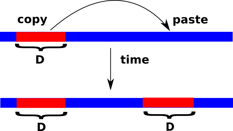
Figure 1: The figure represents random duplications as they appear in the synthetic sequence. A random sequence of the fixed length $D$ (red bar) is chosen from the chromosome (blue bar) and copied into another randomly chosen place of the chromosome thus producing a pair of exact matches. Simultaniously point substitutions are applied to the whole chromosome with some rate. Length distributons of such pairs (with restrictions layed by mummer) is computed and analyzed throughout the paper.

We consider a synthetic chromosome (blue bar in fig. 1) represented as a string of $L$ bases chosen from a finite alphabet; in natural genomes the alphabet consists of four bases A, G, C, and T. The distance between bases is a length scale denoted by $a$; for natural genomes it is close to $1\AA$.

Within our models a subsequence of length $D$ (red bar in fig. 1) is chosen randomly within the chromosome and is substituted for a sequence of length $D$ at another randomly chosen position in the chromosome (fig. 1). These duplications are assumed to occur with the rate $\lambda$ measured per time unit, per base. Simultaniously point substitutions are applied to the system with the rate $\mu$ per time unit, per base.

The sequence feature that we study is the set of repeated sequences within the chromosome. For finding all pairs of exact matches in the synthetic sequence we apply mummer. Mummer searches for maximal repeats or maxmersfootnote2 which are akin to supermaxmersfootnote3-1 mentioned in the previos section and used in koroteev_arxiv in the sense that computation of both sets is based on some maximality condition. However, the set of exact matches computed by mummer is larger than the set of supermaxmers of the same length as the definition of the latter includes additional restrictions. Then the observations show that the output of these computations is noticeably different if we compare the length distributions obtained in the models ardnt and koroteev_arxiv . Our aim here is the model capable to reproduce the simulated length distributions obtained with mummer without any additional restriction as well as an equation for the simulated length distributions. In the discussion below it is always implied that mummer is used with the option -maxmatch which according to the mummer manual produces computations of exact matches ‘regardless of their uniqueness’mummer_manual . The Appendix section also contains more rigorous definitions of various types of repeats. However for the purposes of the analytic derivation suggested below it is sufficient to think that the equations aim to reproduce the length distributions constructed for the set of repeats obtained by mummer, a standard tool in comparative analysis of long DNA.

III Analytic treatment

Let the number of pairs of duplicates of the length $m$ at time moment $t$ is $g_{2}(t,m)$. We assume that new duplication events occur with the rate $\lambda$ per base, per time unit; at the same time the chromosome undergoes point mutation events occurring with the rate $\mu$ per base, per time unit. We first write down the evolutionary (balance) equation for the average number of pairs of duplicates $g_{2}$, which was derived in koroteev_arxiv ; it has the form

$$\frac{\Delta g_{2}}{\Delta t}=-2\left[(m+D-a)\frac{a\lambda}{D}+\mu m\right]g_{2}(t,m)+$$

$$+4\left(\frac{a^{2}\lambda}{D}+a\mu\right)\sum_{k=m+1}^{D}g_{2}(t,k)+L\frac{a\lambda}{D}\delta_{c}(D-m).$$ (1)

The main difference between this equation and the equation of koroteev_arxiv is notation (we use $g_{2}$ here instead of $f$). In addition, there is no prefactor $2$ in the last term of the equation because in koroteev_arxiv we studied the number of duplicated sequences while here we look at the number of pairs of duplicates; thus, the source produces one pair of duplicates at each time step. We also confine ourselves to the equation for the monoscale source using Kronecker delta function $\delta_{c}(D-m)$; different source terms are also possible and will be presented elsewhere. Thus the equation (1) is provided for the reference and connection to the subsequent discussion.

We will then focus on the stationary version of the equation implying that when $t\to\infty$ $g_{2}(t,m)\to g_{2}(m)$ (this can be demonstrated by analytic calculation)

$$0=-2\left[(m+D-a)\frac{a\lambda}{D}+\mu m\right]g_{2}(m)+$$

$$+4\left(\frac{a^{2}\lambda}{D}+a\mu\right)\sum_{k=m+1}^{D}g_{2}(k)+L\frac{a\lambda}{D}\delta_{c}(D-m).$$ (2)

Now in the same way as we looked at pairs of identical duplicates we can look at triplets, quadruplets, etc. of identical sequences and write down the corresponding equations for them. For $i$-plets we will have the following stationary equation

$$0=-i\left[(m+D-a)\frac{a\lambda}{D}+\mu m\right]g_{i}(m)+2i\left(\frac{a^{2}\lambda}{D}+a\mu\right)\sum_{k=m+1}^{D}g_{i}(k)$$

$$+(i-1)\left(\frac{a\lambda}{D}(D-m+a)\right)g_{i-1}(m)+2(i-1)\frac{a^{2}\lambda}{D}\sum_{k=m+1}^{D}g_{i-1}(k),\;i>2$$ (3)

We see that unlike the equation for duplicates containing the source term with the delta function in it, other equations also have sources of new $i$-plets ; these sources are $i-1$-plets and expressed by the last two terms in (3). One produces $i$-plicates of $i-1$-plicates of the same length $m$ (the first term in the second line of (3)); the other generates $i$-plicates of longer $i-1$-plicates by copying and pasting their parts of the length $m$ (the second term in the second line of (3)), i.e., new duplicates, $g_{2}(m)$ generated by the source, in turn produce triplicates $g_{3}(\tilde{m})$, where $\tilde{m}\leq m$, triplicates produce quadruplicates $g_{4}$ etc. The first term in the first line of (3) is responsible for the destruction of sequences by new duplications and point mutations; coefficients represent the corresponding rates. The second term in the first line of (3) shows that longer sequences are turned into shorter ones, again, by duplications and point mutations. The general mechanism has much in common with models studied in fragmentation theoryben-naim . This similarity is also discussed below.

Thus for each $m=1\ldots D$ we have a set of equations for various sets of identical repeats (maxmers). As it was demonstrated in koroteev_arxiv the equation for $g_{2}$ fits well to the length distribution of supermaxmers computed for the synthetic chromosome after applying evolutionary duplication-mutation dynamics described above. Equations for different types of repeats, to our knowledge, were not obtained earlier. We refer to this set of equations as chain because as it is easily seen functions $g_{i}$ represented in the $i$-equation are related to the “adjacent” functions $g_{i-1}$ and $g_{i+1}$.

Using these equations we can obtain the equation corresponding to the length distributions of exact matches computed by mummer as follows. We sum up all the equations for $g_{i}$, $i=1,2,\ldots$ and find a new equation for the function $G(m)=\sum ig_{i}(m)$; the equation has the form

$$-(\zeta+2)mG(m)+2aG(m)+2(\zeta+2)a\sum_{n>m}G(n)+$$

$$+L\delta_{c}(D-m)=0,$$ (4)

where $\zeta=D\mu/a\lambda$ is a dimensionless parameter.

Now we can compare the results of the simulations with the solutions of (4); the comparison is represented in fig. 2.

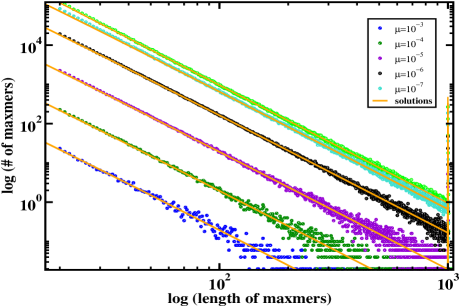
Figure 2: Curves represent stationary length distributions obtained from simulations of duplication-mutation dynamics described in the previous section with a monoscale source for various base substitution rates $\mu$ and corresponding analytic solutions (orange) of (4). The chromosome length $L=10^{6}$; source length $D=10^{3}$, duplication rate $\lambda=10^{-4}$; for simulations we always take $a=1$. Length distributions for the same dynamics computed by mummermummer were obtained using the following options -maxmatch -n -b -l 20. The results were then averaged over $10^{2}$ realizations.

Additional comparisons for different sets of parameters are given in supplemental figures (see Supplemental materials).

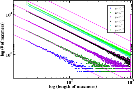
Figure 3: Curves represent stationary length distributions obtained from simulations of duplication-mutation dynamics with a monoscale source for various base substitution rates $\mu$ and corresponding analytic solutions (magenta curves) of eq. (5) of ardnt . All parameters for the simulations and the equation are the same as for fig. 2. The results of simulations were averaged over $10^{2}$ realizations.

Let us now compare solutions of the equation presented in ardnt with the simulations of the same duplication-mutation dynamics. For that we used equation (5) of supplemental materials of ardnt . Comparisons are represented in fig. 3. The solutions of ardnt provide a good agreement for sufficiently large mutation rates compared to the duplication rate $\lambda$ but fail to reproduce the amplitude of the length distributions for different regimes. In this regime saturation is observed wrt. the amplitude of the length distributions which is reproduced by solutions (4) as seen in fig. 2 and supplemental figures 1 and 2footnote6 .

One then can easily understand the qualitative correspondence of length distributions observed in ardnt and koroteev_arxiv for high mutation rates: the growth of mutation rate $\mu$ evidently affects $g_{i}(m)$ for larger $i$ as the growth of $i$ means more sequences in the set which are destroyed faster affected by mutations. Thus the main contribution to $G(m)$ for high mutation rates comes from $g_{2}(m)$ , i.e., $G(m)\sim g_{2}(m)$ as $\zeta\to\infty$ and the dynamics is described by (2) in the main order. Also it is instructive to note that the situation $\mu\gg\lambda$ generally implies $\zeta\gg 1$ and one can neglect in (4) all terms compared to those containing $\zeta$ and the source term with delta function to keep the algebraic tail, hence $L/a$ has to grow as $\sim\zeta$ to keep the same order of the source term $\delta_{c}(D-m)$, otherwise the tail disappears as it is seen from fig. 2 for large $\mu$: here $\zeta$ is growing but the length $L$ remains fixed. However this is not applicable even for $\zeta\sim 1$. On the other hand, if $\mu\ll\lambda$ then $\zeta\to 0$ and we can write down the equation corresponding to the limit of absent mutations as $\zeta$ becomes negligible compared to $1$.

$$-2mG(m)+2aG(m)+4a\sum_{n>m}G(n)+L\delta_{c}(D-m)=0.$$ (5)

If $D$ is fixed as in figs. 2, 3, then the limit amplitude of the algebraic tail is controlled by the only parameter $L$ and all distributions with decreasing $\zeta$ asymptotically have the saturation line; this line establishes an upper boundary for fitting the model to the natural sequence. This also can be seen from the exact solution of (5) that has the form

$$G(m)=\left\{\begin{aligned} \frac{aDL}{(m-a)m(m+a)},\;&m<D\\ \frac{L}{2(D-a)},\;&m=D\end{aligned}\right.$$

with obvious main order term $\sim 1/m^{3}$ as $a\ll m$. The solution is applicable if $a\ll D\ll L$; otherwise finite size effects turn out to be strong.

The existence of saturation also can be viewed from the continuum limit of the dynamics under consideration. Introducing dimensionless variables

$$\bar{a}=\frac{a}{D},\;\bar{m}=\frac{m}{D},\;\bar{L}=\frac{L}{D},$$

so that $D$ corresponds to $1$, we see that the dimensionless size of the lattice $\bar{a}\ll 1$ and hence $\bar{a}\to 0$. We then denote $\bar{m}=x$ and taking into account that $L/D\gg 1$, we also take $\bar{L}\to\infty$; other parameters may vary. Then $\bar{L}\delta_{c}(1-x)$ turns into Dirac delta and the equation (4) takes the form

$$-(\zeta+2)xG(x)+2(\zeta+2)\int_{x}^{\infty}G(y)dy+\delta(1-x)=0.$$

This equation corresponds to the stationary form of eq. (1) in ben-naim . Its solution is

$$G(x)=\frac{1}{\zeta+2}\left[\frac{\delta(1-x)}{x}+\frac{2}{x^{3}}\right].$$ (6)

The function has the exponent $-3$ for all $x\in(0,1)$. It is seen that the apmplitude of the distribution $G(x)$ is controlled by the parameter $1/(\zeta+2)$, while the slope remains the same, but in new variables $\zeta$ has the form $\mu/\lambda\bar{a}$ and as in the continuum limit $\bar{a}\to 0$ the tail $-3$ vanishes unless at least $\mu/\lambda\sim\bar{a}$. For small $\zeta$ the dependence of the amplitude on the parameters $\mu$ and $\lambda$ disappears which corresponds to the observed saturation.

IV Comparison to natural data

For the comparison of our results with natural data we take C. elegans chromosome 2, for which we show the length distribution of exact matches on fig. 4.

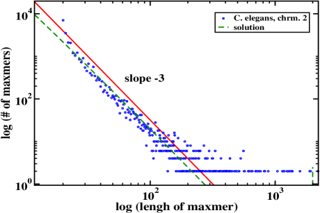
Figure 4: The length distribution for repeat-masked C. elegans chromosome $2$ was computed using mummer with the options -maxmatch -n -b -l 20; self-hits were removed from the distribution. The length of the chromosome is $\sim 10^{7}$. The dotted curve represents the solution of eq. (4) for the parameters computed for the natural chromosome $D=2000$, $\mu=2\times 10^{-2}$, and $\lambda=2\times 10^{-2}$.

As all synthetic sequences when processed with mummer do not contain “self-hits”, i.e., identical sequences located exactly in the same positions for both copies of the chromosome, the self-hits were also removed from the mummer output for the natural sequence. To estimate the parameters of our model for this chromosome we use the estimate for the duplication rate $0.0208$ per gene, per $1$my(million years) or $\approx 400$ duplications occur in genes per $1$mylynch , as the number of genes in the C. elegans genome is estimated to be around $2\times 10^{4}$choi , or $\beta_{0}=40$ per $1$my for chromosome $2$ of length $\sim 10^{7}$ bases (as the length of the whole genome is taken to be $\sim 10^{8}$ bases); for the rate per base $\lambda_{0}$ we have $\beta_{0}/L_{0}$, where $L_{0}$ are bases in the C. elegans chromosome $2$ belonging to genes. It is known that genes cover around $50\%$ of the whole genome in C. elegans, hence $L_{0}\approx 5\times 10^{6}$. We assume that the duplication rate for non-coding parts of the chromosome $\lambda=\lambda_{0}\sim 10^{-5}$ per base, per $1$my. Then we find that $\lambda L=100$ duplications occur in coding and non-coding parts of C. elegans chromosome 2 per $1$my.

For the mutation rate in C. elegans we accept the estimate $\approx 2\times 10^{-2}$ per base, per $1$mydrake ; one generation $=$ four days. To map the parameters of the natural chromosome to the model we use the estimate for the algebraic tail of the length distribution $2D^{2}\lambda/(\mu m^{3})$. This estimate follows from the prefactor in (6) if we take into account that $x\approx\bar{m}=m/D$ and $a=1$. The amplitude of the distribution for any specific $m$ is estimated directly from the plot. In addition, it is necessary to take into account that $\lambda=\lambda_{model}$ from (6) is related to the duplication rate in the natural chromosome $\lambda_{nat}=10^{-5}$ as $\lambda_{model}=D\lambda_{nat}/a$. From all previous estimates we obtain $D\approx 2000$ and $\lambda_{model}=2\times 10^{-2}$. These estimates yield the solution of eq. (4) shown in fig. 4. The exact matches of the length $>200$ observed in the fig. 4 imply that the realistic source of duplications should have non-zero variance unlike the delta source studied here. However, as it was shown in koroteev_miller2011 , such source does not influence the form of the tail for length distribution.

V Discussion

The solutions of the duplication-mutation dynamics presented in the paper raise a number of questions. For the explanation of heavy algebraic tails observed in length distributions of natural sequences we used the solutions of the equations for $t\to\infty$. In connection with biology it should not be unserstood as an effort to say that natural sequences are in fact in a stationary state. First, the models studied here include only two processes having some analogies with processes in natural DNA. Therefore it would not be correct to interpret them as the models of how natural sequences have been varying in their history de facto. For example, in koroteev_miller2011 we demonstrated that long range correlations detected in natural DNA were not found in the synthetic sequences obtained by means of these models; i.e., the length distributions merely reflect some important evolutionary features of natural DNA neglecting other features. Second, it is necessary to stress that basic assumptions of the model imply uniform mutation and duplication rates both in time and in space while in natural genomes these quantities may vary depending, e.g., on the function of a DNA region. Nevertheless the correspondence of the solutions to the model and natural data demonstrates that the equations detect essential details of the data. On the other hand, it is hardly possible to indicate a characteristic time scale for all eukariotic sequences on which significant evolutionary changes occurred to form the modern genomes. Therefore, as the time for natural sequences is restricted by the present moment, we do not have sufficient evidence to map this time moment to a specific time moment of the model and the most plausible assumption is to map it to the stationary state of the model attained for $t\to\infty$ (in the units of the model). This assumption is confirmed by observations that stationary length distributions of the model reproduce the length distributions of natural sequences. However, this should be rather understood as a sojourn of a non-stationary solution in the neighbourhood of the stationary one sufficiently long time compared to a characteristic time scale in the system rather than a “fixation” of natural genomes in stationary states and thus the stationary system approximates well the natural DNA while the latter still may remain non-stationary. Obviously, if a natural chromosome demonstrates noticeable deviations from algebraic tail or other deviations from stationary solution, the assumption of non-stationarity becomes possible and has to be studied separately.

The equations (4) have several features deserving to be stressed. First of all, the equations we derived for $G(m)$ allow the length distributions of exact matches computed by mummer in a broad range of parameters to be reproduced correctly. That means, in part, that histograms computed by counting pairs of maximal exact matches with mummer can be understood as $\sum ig_{i}(m)$ i.e., they represent a cummulative sum of all sequences of duplicates, triplicates, etc. It is worth noting that the mummer output does not compute functions $g_{i}(m)$ directly and thus the question of interpretation of $g_{i}$ in terms of biologically meaningful sequences remains open: we observe only some cumulative effect of distributions for $g_{i}(m)$. On the other hand, the correspondence of functions $g_{2}(m)$ to the length distribution of supermaxmers indicates a potential way to resolve this issue: if functions $g_{2}(m)$ were interpreted as supermaxmers then the candidates for $g_{3}(m)$, $g_{4}(m)$ etc. could be so called ‘local maxmers’taillefer2014 ; footnote5 . At the same time the observed correspondence of mummer output and the function $G(m)$ suggests we have an analytic interpretation for the length distributions computed by mummer for natural sequences: the length distributions for natural sequences exhibiting algebraic behaviour with the exponent $-3$ can be understood in terms of equations (3) and (4) and their solutions.

The representation $G(m)=\sum_{i}ig_{i}(m)$ also indicates that the function $G(m)$ for each $m$ can be thought of as average number of sequences $\bar{i}$ if $g_{i}(m)$ implies a non-normalized distribution function of the number of sequences per one exact match over $i$. The equation (4) has the form of a fragmentation equation with an input and thus can be construed as stationary fragmentation equation of these average quantities $G(m)$.

We also proposed a hierarchy of equations for $g_{i}$; the first of these equations, i.e, for $g_{2}$, was derived in koroteev_arxiv and we see that the equations of ardnt and koroteev_arxiv as well as those presented here treat different subjects focusing on various restrictions imposed on exact matches; in part, the work in koroteev_arxiv deals with the collection of ‘supermaxmers’, specific pairs of exact repeats computed with additional conditions of maximality which are discussed intaillefer2014 (see Appendix 1); they are important as the equations for them not only account for the observed algebraic behaviour in length distributions of natural DNA sequences but demonstrate, in part, non-algebraic length distributions also observed both in simulations and natural DNA and also because their definition provides them with a natural biological interpretationtaillefer2014 . They are accounted for by equation (2) and demonstrate obvious discrepancy from the length distribution of exact matches (suppl. fig. 3). Our equation (4) treats all pairs of exact matches neglecting their uniqueness and reproduces their length distributions. Then $G(m)$ in our interpretation may be represented as a sum of ‘supermaxmers ’for which the biological interpretation was already discussed and other sets of sequences obtained by natural extension of the concept of supermamxers; in this sense, we expect that such an interpretation of $g_{i}(m)$, $m>2$ will appear soon.

The author is acknowledged to Kun Gao for helpful discussion.

VI Appendix 1. To the definition of excat matches

In the appendix we provide more rigorous definitions of maximal repeats or matches which were used in the paper but which allow to distinguish the results presented here from those obtained earlier. There may be several approaches to the definition of exact matches and supermaximal repeats (cf. taillefer2014 ); our approach construes the sequence as a set and thus all definitions are given in terms of sets and subsets.

§1. Consider a finite sequence of objects $x_{i}$, $i=1,2\ldots L$, $L<\infty$. For each element of the sequence there is a pair $\{i,x_{i}\}$, where $i$ is the number of an element in the sequence; hence, we have a set of pairs $\{i,x_{i}\}_{i=1}^{L}$. We denote this set by $X$. By $X_{k}$ we denote a subset of $X$ consisting of $k$ pairs $\{i,x_{i}\}$corresponding to $k$ consecutive elements of the sequence. In the case of DNA sequences the sequence of the length $L$ corresponds to the whole chromosome, or whole genome or even any long DNA sequence.

§2. The configuration space is defined by possible values of $x_{i}$. In general situation we can assume that this space $S$ is the same for all sites of the sequence and $S=\{0,1,2,\ldots,N-1\}$. Thus, we have $N^{L}$ possible states of the system. Consider also the set $Y$ of all arbitrary $N$-ary sequences containing $1\leq l\leq L$ elements. This is a finite set with the cardinal number $\left|Y\right|=\sum_{k=1}^{L}N^{k}=N(N^{L}-1)/(N-1)$. Elements of this set will be denoted by $y_{k}$ where index $k$ implies the number of elements the corresponding sequence. The elements of $y_{k}$ are denoted $y_{k}=(y^{1}_{k},y^{2}_{k},\ldots,y^{k}_{k})$. For DNA sequences the configuration space has the form $S=\{A,C,G,T\}$.

Example. Let the configuration space be binary, i.e., $S=\{0,1\}$. Consider the sequence $\mathfrak{X}=\{10101010\}$ for which $L=8$. The set $X$ is represented as follows

$$X=\{\{1,1\},\{2,0\},\{3,1\},\{4,0\},\{5,1\},\{6,0\},\{7,1\},\{8,0\}\}.$$

For this set one of the $X_{3}$s is given by $\{\{2,0\},\{3,1\},\{4,0\}\}$. The set $Y$ consists of all binary sequences containing $l$ elements, $1\leq l\leq 8$. An example of an arbitrary $y_{4}$ is furnished by an arbitrary binary sequence of $4$ elements.

§3. We say that the element $y_{k}\in Y$ intersects with the sequence $X$ if $\exists a:1\leq a\leq L-k$ such that $y^{j}_{k}=x_{a+j-1}$, $j=1,2,\ldots k$. In our example the element $y_{4}=\{1010\}$ intersects with $X$ three times. The subsets of $X$ corresponding to these intersections are given by $X^{1}_{4}=\{\{1,1\},\{2,0\},\{3,1\},\{4,0\}\}$, $X^{2}_{4}=\{\{3,1\},\{4,0\},\{5,1\},\{6,0\}\}$, $X^{3}_{4}=\{\{5,1\},\{6,0\},\{7,1\},\{8,0\}\}$.

Let the element $y_{k}\in Y$ intersected with $X$ and the intersection is given by the set $\{X^{1}_{k},X^{2}_{k},\ldots X^{r}_{k}\}$. We denote that by $y_{k}=\{X^{1}_{k},X^{2}_{k}\ldots X^{r}_{k}\}$ where $X^{j}_{k}\subset X,\forall j$.

Definition 1. The element $y_{k}=\{X^{1}_{k},X^{2}_{k}\ldots X^{h}_{k}\}\in Y$ is referred to as sub-maximal k-mer if $h>1$.

Definition 1^′. Each pair of sets $(X^{i}_{k},X^{j}_{k})$, $i\neq j$ of $y_{k}$ is referred to as exact match.

Definition 2. Exact match $(X^{i}_{k},X^{j}_{k})$, $i\neq j$ is referred to as maximal exact match if at least one of $X^{i}_{k},X^{j}_{k}\notin X^{s}_{k+p}$ $\forall p\geq 1$ and $\forall s$ such that $X^{s}_{k+p}\in y_{k+p}=\{X^{1}_{k+p},\ldots X^{b}_{k+p}\}$ where $y_{k+p}$ is a sub-maximal $k+p$-mer.

Example.

Consider the sequence

$$TGGT\underline{GGTTA}ATTCACA\underline{GGTTA}CA\underline{GGTTA}GGG$$

Its subsequence $GGTTA$ is a sub-maximal $5$-mer with $h=3$. Each pair of three sequences of it forms an exact match. On the other hand, a maximal exact match is formed by any pair except that, containing the sequences $2$ and $3$ as both these sequences turn out to be immersed into longer sub-maximal maxmer $ACAGGTTA$. This can be expressed in other words by saying that maximal exact matches can not be extended even by one symbols to the left or to the right to remain in the same time exact matches.

§4. For further purposes we should notice that a sub-maximal $k$-mer can be contained into another submaximal $k+p$-mer, $p>0$ in the sense that it may occur that $\forall$ $X^{i}_{k}$ there exists $X^{j}_{k+p}$: $X^{i}_{k}\subset X^{j}_{k+p}$. This observation motivates the following definition.

Definition 3. The sub-maximal $k$-mer $y_{k}=\{X^{1}_{k},X^{2}_{k},\ldots X^{h}_{k}\}\in Y$ is referred to as local maximal k-mer if for any sub-maximal maxmer $y_{k+p}=\{X^{1}_{k+p},\ldots X^{b}_{k+p}\}$, where $p\geq 1$ $\exists X^{i}_{k}\in y_{k}$ such that $X^{i}_{k}\bar{\subset}X^{j}_{k+p}\in y_{k+p}$, $j=1\ldots b$.

Definition 4. A local maximal k-mer is referred to as a super maximal k-mer if the conditions of definition 3 are valid for all $X^{i}_{k}\in y_{k}$.

In the example above the subsequence $ACAGGTA$ represents a supermaximal $7$-mer, while three sequences $GGTTA$ yield a local maxmer, as only the first such sequence can not be extended while two other sequences can be extended to supermaximal maxmer $ACAGGTA$.

It is seen that relations of maximal exact matches and supermaximal and local maximal maxmers are not straightforward. One may roughly say that the set of all supermaximal repeats would be a subset of all maximal exact matches. However insignificant deviations from this inclusion can appear because we define maximal exact matches as pairs of elements while supermaxmers even for DNA sequences can consist of three sequences; but such supermaxmers are so rare that their influence is negligible and in a zeroth approximation we can rely on the relation indicated above. The connections to local maxmers are more subtle: from the example above it is clear that maximal exact matches are often “chosen” as pairs from local maxmers containing many sequences. Though it is correct that supermaximal and local maxmers suggest more non-trivial division of repeats in the chromosome, maximal exact matches as we defined them above provide an independent measure of non-local correlations in DNA.

VII Appendix 2. To the definition of length distribution.

§5. Based on the previous definitions of various repeats we provide more rigorous treatment of the length distribution.

Definition 5. The number of $X^{j}_{k}$ containing in sub-maximal k-mer is referred to as index of the sub-maximal k-mer with respect to the set $X$ and is denoted by ${\rm In}_{X}(y_{k})$.

Thus ${\rm In}_{X}(y_{k})=h$ (cf. definition 1). This obviously would correspond to introducing some indicator function on the set $Y$. According to the definition 1, $\min_{y\in Y}{\rm In}_{X}(y_{k})=2$. In addition, the function ${\rm In}_{X}(y_{k})$ is non-negative and finite-valued. If the element $y_{k}$ is not a sub-maximal k-mer, then we put ${\rm In}_{X}(y_{k})=0$. The index is defined similarly for all types of repeats introduced in §§3,4.

§6. Let us introduce an equivalence relation on $Y$. Two elements of $Y$ are equivalent if they are both sub-maximal $k$-mers wrt. $X$. Thus, the set $Y$ is partitioned into classes of equivalent elements. The set obtained by means of factorization of $Y$ with respect to this equivalence relation is denoted by $Y^{X}_{F}$. Thus, each element $y^{F}_{k}\in Y^{X}_{F}$ consists of all sequences $y\in Y$ of $k$ elements intersecting to $X$ and included to some (sub)maximal $k$-mer.

The notion of index is easily redefined for arbitrary equivalence classes (not only for sub-maximal k-mer but for maximal exact matches or supermaxmers). These definitions are straightforward and we omit them.

Definition 5’. If $y^{(1)}_{k},y^{(2)}_{k}\ldots,y^{(p)}_{k}\in Y$ are equivalent with respect to the equivalence relation $F$, then the index of the corresponding element $y^{F}_{k}\in Y^{X}_{F}$ is given by

$${\rm In}(y^{F}_{k})=\sum_{i=1}^{p}{\rm In}_{X}(y^{(i)}_{k}).$$ (7)

§7. Example. We can consider the notion of index in application specifically to supermaxmers. In this case the configuration space is $S=\{A,T,C,G\}$ and supermaximal maxmers can contain $2,3$ or $4$ sequences. Thus, according to definition 5 the corresponding indexes are equal to $2,3$ and $4$. The space $Y^{X}_{F}$ is obtained by establishing the equivalence of all supermaxmers, which have the same number of elements.

The complete number of elements containing in $y^{F}_{k}\in Y^{X}_{F}$ is given by (7). As each $y\in Y$ belongs to at least one $y^{F}_{k}$, then $Y$ is partitioned into equivalence classes with respect to supermaximal sequences. Consequently ${\rm In}(y^{F}_{k})$ can be computed for any $y^{F}_{k}$. Then we can introduce the following definition.

Definition 6. The function $n(k)={\rm In}(y^{F}_{k})$, $y^{F}_{k}\in Y^{X}_{F}$, $k=1,2,\ldots$ is referred to as empirical length distribution on $Y$ wrt. $X$.

§8. It is important to notice that the equivalence relation is constructed for studying some correlation properties of m-ary sequences, e.g., genomes, which do not depend on a concrete structure or content of these sequences but which would incorporate physical length as one of the governing parameters. In this context it should be understood that there are many other ways to construct an equivalence relation or, in physical terms, coarse graining on $Y$. However, these definitions typically neglect the physical length. The simplest way is to include only supermaximal $k$-mers and neglect local ones. To give a less obvious and exotic example we may say that two elements of $Y$ are equivalent if, provided that configuration space is $S=\{0,1\}$, they contain equal fractions of 1s. This is especially easy to envisage for binary sequences but also may be reasonable for arbitrary m-ary sequences. In part, the similar construction was applied in lee to produce so called $k$ spectra of genomes. As genetic ’alphabet’ consists of $4$ letters the authors consider $k$-mers with respect to the fraction of (A+T) content. In our terms that means introducing a different equivalence relation on the set $Y$ than one mentioned above. On the other hand, we may consider the trivial equivalence relation when any $y\in Y$ is equivalent only to itself. This situation is ubiquitously exploited, e.g., in genomics where one can take a specific “functional” sequence and ask whether its copies are found in different genomes. In this situation the content of the sequence is not eliminated because the assumed functionality implies that any nucleotide may be important. The interesting example of manipulations with this limiting case of self-equivalency is given in lee .

Supplemental Materials: On a chain of fragmentation equations for duplication-mutation dynamics in DNA sequences

VIII Supplemental figures

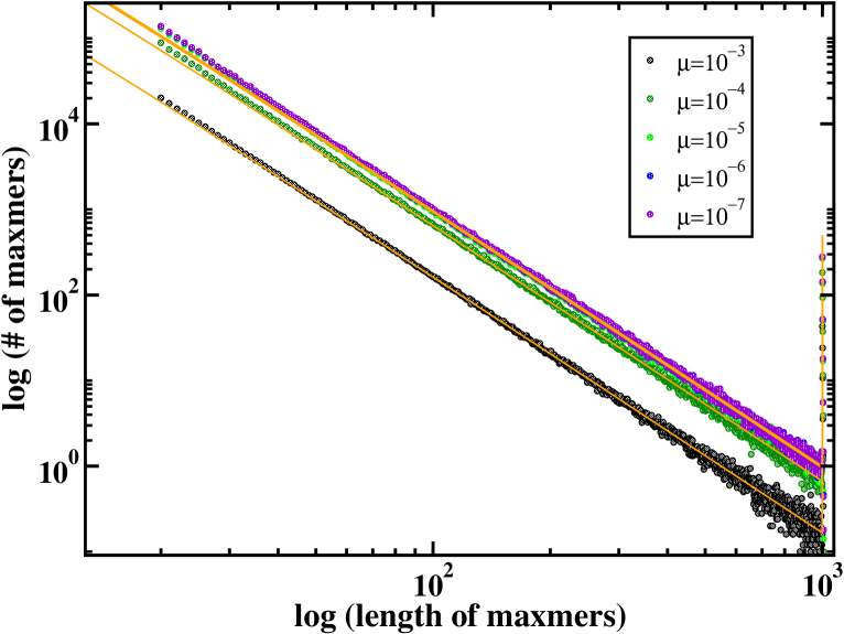
Figure S1: Comparisons of simulations with solutions of equation (4) of the main text. The parameters are: $L=10^{6}$, $D=10^{3}$, $\lambda=10^{-1}$. Empirical length distributions were computed with the same switches of mummer as indicated in the caption for figure 1 of the main text. The distributions were averaged over $100$ realizations.

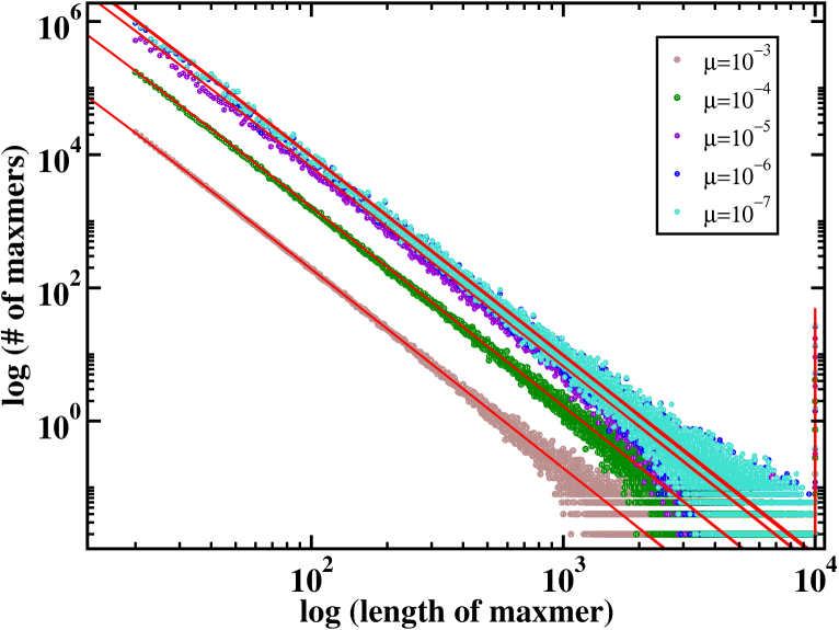
Figure S2: Parameters of the model are: $L=10^{6}$, $D=10^{4}$, $\lambda=10^{-1}$. All other parameters and options are the same as in figure 1 of the main text and supplemental figure 1.

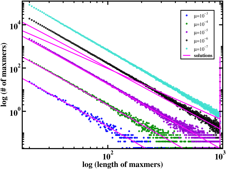
Figure S3: Length distributions obtained with duplication-mutation dynamics using mummer with the parameters -n -b -l 20. Parameters of the model are: $L=10^{6}$, $D=10^{3}$, $\lambda=10^{-4}$ and correspond to those indicated in the fig. 1 of the main text. Magenta curves represent the solutions of the equation (2) of the main text.

References

- (1) M.V. Koroteev, J. Miller. Phys. Rev. E 84, 061919 (2011)
- (2) F. Massip, P.F. Arndt, Phys. Rev. Lett. 110, 148101 (2013).
- (3) M.V. Koroteev, J. Miller. Fragmentation dynamics of DNA sequence duplication, preprint. arXiv:1304.1409v1
- (4) The applications of length distributions in genomics have a long history (see sawyer ; altschul ). For the purposes of this paper a length distribution of matches or maxmers can be thought of as a histogram which has the length of maxmer on -axis and the number of pairs (or triplets etc.) of identical matches on -axis. We normally plot all length distributions in double log scale. An approach demonstrating relations of length distributions to various types of repeats is developped in koroteev2015 .
- (5) S. Sawyer. Mol. Biol. Evol. 6(5), (1989).
- (6) S.F. Altschul, W. Gish, W. Miller, E.W. Myers, D.J. Lipman. J. Mol. Biol. 215(3), (1990).
- (7) M.V. Koroteev. arXiv:1501.04078.
- (8) W. Salerno, P. Havlak, J. Miller, Proc. Nat. Acad. Sci. USA, 103:13121 (2006).
- (9) J. Miller, IPSJ SIG Technical Report No. 2009-BIO-17(7):1 (2009).
- (10) K. Gao and J. Miller, PLoS One 6(7), (2011).
- (11) There are multiple terms in the literature for exact copies of parts of DNA sequences; sometimes they are simply referred to as exact matches, in other cases it is thought to be important that exact matches are not contained in longer exact matches: in the latter case the term maxmers is used. Exact matches also can be referred to as exact repeats.
- (12) E. Taillefer, J.Miller. J. Bioinformatics Comp. Biol. 12(1), 2014.
- (13) E. Taillefer and J. Miller, in Proceedings of International Conference on Natural Computation, Shanghai, China, 2011, Vol. 3 (IEEE, New York, 2011), pp. 1480–1486.
- (14) S. Kurtz, A. Phillippy, A.L. Delcher, M. Smoot, M. Shumway, C. Antonescu, and S.L. Salzberg, Genome Biology (2004), 5:R12.
- (15) both types of repeats include a condition of maximality of exact matches; this condition, however, turns out to be insufficient to obtain similar length distributions.
- (16) http://mummer.sourceforge.net/manual/#maximal
- (17) E. Ben-Naim, P.L. Krapivsky, Phys. Lett. A, 293(48), 2000. See also E. Ben-Naim, P.L. Krapivsky, J. of Statistical Mechanics theory and experiment, DOI: 10.1088/1742-5468/2005/10/L10002, 2005.
- (18) In the context of fig. 3 it is necessary to stress that computations of ardnt are different from those presented here as the authors of ardnt use additional post-processing of mummer output as it is seen from the page 2 of supplemental materials of ardnt . Therefore fig. 3 does not try to argue with the conclusions of ardnt but only that these are different dynamics.
- (19) M. Lynch, J.S. Conery. Science, 290, 1151(2000).
- (20) J. Choi, A. Newmann. Develop. Biol., 296(2006), 537-544
- (21) J.W. Drake, B. Charlesworth, D. Charlesworth, J.F. Crow. Genetics, 1998 Apr148(4):1667-86. p.1673 Table 5.
- (22) Resolution of this issue will become possible when the software for computation of local maxmers will have been publicly available. The task of local maxmers computation and analysis is nontrivial and is out of the scope of the paper.
- (23) S.-G. Kong, W.-L. Fan, H.-D. Chen, J. Wigger, A.E. Torda, and H.-C. Lee, Phys. Rev. E 79, 061911(2009)