Optimizing information flow in small genetic networks.
IV. Spatial coupling

Abstract

We typically think of cells as responding to external signals independently by regulating their gene expression levels, yet they often locally exchange information and coordinate. Can such spatial coupling be of benefit for conveying signals subject to gene regulatory noise? Here we extend our information-theoretic framework for gene regulation to spatially extended systems. As an example, we consider a lattice of nuclei responding to a concentration field of a transcriptional regulator (the “input”) by expressing a single diffusible target gene. When input concentrations are low, diffusive coupling markedly improves information transmission; optimal gene activation functions also systematically change. A qualitatively new regulatory strategy emerges where individual cells respond to the input in a nearly step-like fashion that is subsequently averaged out by strong diffusion. While motivated by early patterning events in the Drosophila embryo, our framework is generically applicable to spatially coupled stochastic gene expression models.

I Introduction

Signals encoded by spatial or temporal concentration profiles of certain proteins play a crucial role in communicating information within and between cells. Such signals are established and read out by a vast variety of gene regulatory networks. In this process, however, information flow is limited by the randomness associated with gene regulatory interactions—essentially chemical reactions between different species of signaling molecules and DNA—taking place at very low copy numbers van Kampen (1981). While we increasingly understand distinct strategies of noise control in biological systems Tsimring (2014); Lo et al. (2015); Zhang et al. (2012); Eldar et al. (2004, 2002), it remains largely unclear how nature orchestrates these strategies to maximize information flow.

A recent proposal takes the idea of “information flow” in biological networks seriously, as formalized by Shannon’s information theory, and hypothesizes that at least some of the structure of genetic regulatory networks could be derived mathematically, by maximizing information transmission that such networks can sustain subject to biophysically realistic constraints Tkačik and Walczak (2011). The feasibility of information as the metric of network performance was recently established by demonstrating that morphogen patterns in early fly development transmit information with an accuracy close to the physical limits Tkačik et al. (2008a); Dubuis et al. (2013a). Theoretically, this optimization principle was applied to study information flow in different paradigmatic gene-regulatory scenarios, including single and multiple target genes regulated by a single input Tkačik et al. (2008b, 2009); Walczak et al. (2010), feed-forward cross-regulation Walczak et al. (2010), autoactivation Tkačik et al. (2012), multistate promotor-switching Rieckh and Tkačik (2014), and time-dependent inputs Tostevin and ten Wolde (2009, 2010); de Ronde et al. (2010); Mugler et al. (2010); Selimkhanov et al. (2014). These attempts yielded important insights into optimal strategies with which single cells can reliably respond to external stimuli. The issue that to-date has not received attention, however, is that many cells or nuclei can respond to a spatially distributed signal collectively, by exchanging information among themselves, e.g., via diffusion of signaling proteins. Prominent examples are the specification of emerging body tissues during embryo development Jaeger (2011); Jaeger et al. (2012); Rushlow and Shvartsman (2012); Restrepo et al. (2014); Wartlick et al. (2009); Meinhardt (1982), the aggregation response in colonies of amoebae Gregor et al. (2010); Kamino et al. (2011), and collective chemosensing in cell colonies and tissues Sun et al. (2012, 2013). Importantly, spatial aspects not only add another layer of complexity to the distributions of input and output signals of gene-regulatory networks; they can also markedly alter noise levels—and thus information capacity—through spatial averaging Erdmann et al. (2009); Sokolowski et al. (2012); Little et al. (2013); Garcia et al. (2013); Mugler et al. (2014); Tikhonov et al. (2014). A truly predictive theoretical framework therefore must take into account the spatial setting, where multiple regulatory networks can read out the inputs at various locations and exchange information between themselves locally.

Here we extend the existing theory of optimal gene regulatory networks to such a spatial setting. We construct a spatial-stochastic model of gene regulation that takes into account diffusive coupling between neighboring reaction volumes and the relevant sources of noise. We derive simple expressions for the stationary means and variances of input-activated local protein levels as a function of their regulatory parameters and diffusion rate. From this we compute information transmission in various spatial scenarios and systematically explore how transmission can be optimized by changing key system parameters. As a motivating example, we study a model variant representative of the bicoid-hunchback system in early fruit fly embryogenesis, which enables differentiating cells to acquire position-dependent fates with high reliability and reproducibility in spite of stochasticity in the underlying biophysical processes Houchmandzadeh et al. (2002); Gregor et al. (2007a, b); Dubuis et al. (2013b); Little et al. (2013); Petkova et al. (2014); Manu et al. (2009); de Lachapelle and Bergmann (2010). Our approach thus specifically optimizes positional information, a notion that has been extensively discussed throughout developmental biology Wolpert (1969, 1994, 1996, 2011); Hironaka and Morishita (2012), but only recently rigorously formalized in mathematical terms, using information theory Tkačik et al. (2015); the proposed formalism, however, generalizes to other spatially coupled gene regulatory setups.

We find that spatial coupling can markedly improve information transmission when the dominant source of noise in gene regulation is on the “input side,” e.g., due to the random arrival of the regulatory molecules (transcription factors) to their binding sites on the DNA. This is in accordance with the known fact that spatial averaging can remove super-Poissonian contributions to the noise Erdmann et al. (2009); Sokolowski et al. (2012). Moreover, with diffusion the maximal information capacity reached upon optimization becomes increasingly invariant to the spatial details of the input signal. Finally, in a defined noise regime that we detail below, we observe the emergence of a novel optimal regulatory strategy where diffusion generates graded, and thus informative, spatial profiles of regulated genes despite their sharp, threshold-like activation by the regulatory inputs.

II Methods

Here we construct a model in which we can analytically calculate how much information expression levels of diffusible proteins encode locally about the position itself, if these proteins are expressed in response to a concentration field of regulatory input molecules. The outline of our approach is as follows. We (i) define a generic spatial-stochastic model of gene regulation that explicitly accounts for diffusive signaling between adjacent volumes which collectively interpret a spatially distributed input signal (Section II.1). Starting from a set of coupled Langevin equations, in Section II.2 we (ii) derive general analytic expressions for the stationary means and variances of the regulated protein levels, and provide intuitive insight for the role of diffusion prior to specifying any gene regulatory details. We then (iii) impose realistic expressions for the gene regulatory function and noise, based on well-established biochemical models (Section II.3). Section II.4 illustrates how we (iv) quantify the encoding of positional information, using information theory and the stationary moments derived in (ii). Finally, we vary the parameters of the model to find the optimal regulatory strategies in the spatially coupled setup, which we present in the “Results” Section III.

II.1 Spatial-stochastic model of gene regulation

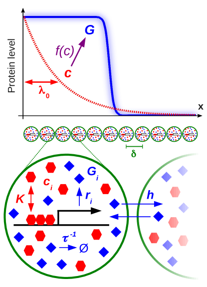
Figure 1: Model schematic. The spatial-stochastic model of gene regulation consists of a discrete set of identical reaction volumes (indicated by $i$) arranged in a regular lattice with lattice spacing $\delta$. While here for clarity we only draw a 1D lattice, we also study a 2D model with periodic boundary conditions, and our framework supports arbitrary coordination numbers. The volumes collectively sense a spatial signal $c(x)$ which maps the position $x$ to an input concentration $c$ (red), creating a spatial distribution of output proteins $G$ (blue). Each volume contains an identical promotor activated with probability $f(c_{i})$, where $f(c)$ is the regulatory function and $c_{i}$ the activator concentration in volume $i$. This results in a local production rate $r_{i}=r_{\rm max}f(c_{i})$ and local levels $G_{i}$ of the product protein. $G$ proteins are degraded with a rate $1/\tau$ and can hop to the neighboring volumes with a rate $h=D/\delta^{2}$, where $D$ is their diffusion coefficient. The regulatory function $f(c)$ is characterized by the activation threshold $K$ and the regulatory cooperativity $H$, as detailed in Section II.3.

Figure 1 shows a schematic of the spatially coupled gene regulation model that we study throughout this paper. We consider a two-dimensional lattice of $N_{x}\times N_{y}$ reaction volumes with equal spacing $\delta$ between the volumes. In this work, we particularly focus on a cylindrical geometry of the lattice, with periodic boundary conditions along the circumference ($y$-direction), and reflective boundary conditions in axial ($x$-) direction. While this geometry deliberately mimics the syncytial state of the developing embryo of the fruit fly Drosophila, our model could be easily adapted to any arbitrary discrete arrangement of equally spaced reaction volumes. We will initially consider the special case $N_{y}=1$ as the “1D model,” while referring to the case $N_{y}>1$ as the “2D model.”

Each volume contains the promotor of an identical gene controlled by a single transcription factor, whose concentration we denote by $c$. The copy number of proteins expressed from this gene of interest will be denoted by $G$, while $g=G/N_{\rm max}$ will refer to the copy number normalized by the maximal average expression level $N_{\rm max}$ at full induction. At the core of our model is the regulatory function $f(c)$ which determines how the activator concentration $c$ maps to the effective synthesis rate of $G$ proteins. We will also refer to $c$ as the “input,” and to $G$ and $g$ as the “output.” For simplicity we treat transcription and translation as a single production step with maximal production rate $r_{\rm max}$ reached at full activation. $G$ molecules are degraded with a constant rate $1/\tau$, where $\tau$ is the average protein lifetime. In addition, each volume can exchange the product molecules $G$ with its neighboring volumes via diffusion. Here, we approximate this exchange with an effective “hopping rate” $h=D/\delta^{2}$, where $D$ is the diffusion coefficient of $G$ molecules.

Denoting the position of volume $i$ by $\mathbf{x}_{i}$, we can write down a stochastic equation for the combined production-degradation-diffusion process in volume $i$ as follows:

$$\partial_{t}G_{i} =r_{\rm max}f(c(\mathbf{x}_{i}))-\frac{1}{\tau}G_{i}$$

$$\qquad\qquad-\frac{D}{\delta^{2}}\sum_{n\in N(i)}(G_{i}-G_{n})+\sum_{k}\Gamma_{ik}\eta_{k}$$ (1)

Here $G_{i}$ denotes the number of $G$ proteins in the volume, while the first and second term in the equation describe their production and degradation, respectively. The third term is a discretized Laplacian accounting for the diffusive exchange of $G$ molecules between volume $i$ and its nearest-neighbor volumes $n\in N(i)$. Function $c(\mathbf{x})$ maps positions $\mathbf{x}_{i}$ to local transcription factor concentrations $c_{i}$. In this work we consider the case in which $c(\mathbf{x})$ is invariant in $y$-direction, i.e. $c_{i}\equiv c(\mathbf{x}_{i})=c(x(i))$; we specify the functional form of $c(x)$ at the end of this section. The noise term $\sum_{k}\Gamma_{ik}\eta_{k}$ comprises all noise sources $\eta_{k}$ that act on the protein level $G_{i}$, including those outside of volume $i$. We assume that all fluctuations are well represented by non-multiplicative, zero-mean Gaussian white noise, and compute the relevant noise powers $\Gamma_{ik}$ below.

II.2 Means and variances with spatial coupling

The set of coupled Langevin equations [Eq. (1)] is a special case of what is known as the “N-unit generalized Langevin model” Hasegawa (2006, 2007) in other contexts. To compute the steady-state means and variances we employ a technique based on Itō calculus which allows to convert the set of coupled stochastic equations for the variables $G_{i}$ into a set of ODEs for their moments that hold exactly. This can be performed for an arbitrary discrete coupling network, and even for the case of multiplicative noise (not considered here) Rodriguez and Tuckwell (1996); Hasegawa (2006, 2007).

We can write down the equations of motion for the mean of the normalized local output $g_{i}=G_{i}/N_{\rm max}$ and the (co)variances of its fluctuations $\delta g_{i}\equiv g_{i}-\langle g_{i}\rangle$ as follows Rodriguez and Tuckwell (1996); Hasegawa (2006, 2007):

$$\partial_{t}\langle g_{i}\rangle =\langle F(g_{i},c_{i})\rangle-h\sum_{n_{i}\in N(i)}\big{\langle}g_{i}-g_{n_{i}}\big{\rangle}$$ (2)

$$\partial_{t}\langle\delta g_{i}\delta g_{j}\rangle =\langle\delta g_{i}F(g_{j},c_{j})\rangle+\langle\delta g_{j}F(g_{i},c_{i})\rangle$$

$$\quad+h\left\langle\delta g_{i}\sum_{n_{j}\in N(j)}(g_{n_{j}}-g_{j})\right\rangle$$

$$\quad+h\left\langle\delta g_{j}\sum_{n_{i}\in N(i)}(g_{n_{i}}-g_{i})\right\rangle$$

$$\quad+\sum_{k}\langle\Gamma_{ik}\Gamma_{jk}\rangle$$ (3)

Here the function $F(g_{i},c_{i})=\frac{1}{\tau}\left(f(c_{i})-g_{i}\right)$ groups the production and degradation terms and depends on the regulatory function $f(c)$. The $n_{i}$- and $n_{j}$-sums run over the nearest-neighbor volumes of $i$ and $j$, respectively. Note that in the $k$-sum running over all noise sources in the system usually most terms will be zero.

The hitherto arbitrary noise powers $\Gamma_{ik}$ can be written out more explicitly by listing all noise sources that affect volume $i$ in the following way:

$$\sum_{k}\Gamma_{ik}\eta_{k}= \mathcal{G}_{i}(c_{i},\mathbf{g})\gamma_{i}$$

$$-\sum_{n\in N(i)}\mathcal{D}_{(i\rightarrow n)}\xi_{(i\rightarrow n)}+\sum_{n\in N(i)}\mathcal{D}_{(n\rightarrow i)}\xi_{(n\rightarrow i)}$$ (4)

Herein $\gamma_{i}$ is the noise in the combined process of random regulation, production and degradation, and $\xi_{(i\rightarrow j)}$ the noise caused by random hopping from volume $i$ to $j$. A crucial step in specifying the expression above is to write the noise powers of the incoming and outgoing hopping processes with different signs, because each hopping event causing a negative fluctuation in the volume of origin always causes a positive fluctuation in the volume of arrival. The hopping thus is a birth process when seen from the volume of arrival, and a death process when seen from the volume of origin. This intuitive argument can be derived more rigorously from the Langevin equation following the method portrayed by Gillespie Gillespie (2000), and is quantitatively confirmed by stochastic simulations, employing (e.g.) the next-subvolume method Hattne et al. (2005); Elf and Ehrenberg (2004).

Using Eq. (4) we can rewrite the noise term $\sum_{k}\langle\Gamma_{ik}\Gamma_{jk}\rangle$ in Eq. (3) for the variances (case $i=j$) and nearest-neighbor covariances (case $i\in N(j)$) as follows:

$$\sum_{k}\left\langle\Gamma_{ik}\Gamma_{jk}\right\rangle =\langle\mathcal{G}_{i}^{2}(c,\mathbf{g})\rangle+\sum_{n\in N(i)}\langle\mathcal{D}_{(i\rightarrow n)}^{2}+\mathcal{D}^{2}_{(n\rightarrow i)}\rangle$$

$$\equiv\mathcal{N}^{2}_{ii}\qquad\qquad\qquad\qquad\text{for }i=j$$ (5)

$$\sum_{k}\left\langle\Gamma_{ik}\Gamma_{jk}\right\rangle =\underset{\text{hopping }(i\rightarrow j)}{\underbrace{\left\langle\Gamma_{i\kappa}\Gamma_{j\kappa}\right\rangle}}+\underset{\text{hopping }(j\rightarrow i)}{\underbrace{\left\langle\Gamma_{i\kappa^{\prime}}\Gamma_{j\kappa^{\prime}}\right\rangle}}$$

$$=-\langle\mathcal{D}^{2}_{(i\rightarrow j)}\rangle-\langle\mathcal{D}^{2}_{(j\rightarrow i)}\rangle$$

$$\equiv\mathcal{N}^{2}_{ij}\qquad\qquad\qquad\qquad\text{for }i\in N(j)$$ (6)

To obtain the stationary means and covariances of the protein number $g_{i}$, we solved Eqs. (2) and (3) in steady state by setting their left sides to zero ($\partial_{t}\langle..\rangle=0$). After substituting $g_{i}=\langle g_{i}\rangle+\delta g_{i}$, we regroup covariances $\langle\delta g_{i}\delta g_{j}\rangle$ and means $\langle g_{i}\rangle$ and relate them to the respective quantities in the neighboring volumes (see Appendix A). In this context, we introduce the pragmatic assumption that only concentrations in volumes that are nearest neighbors on the lattice have significant correlations, i.e., we enforce

$$\langle\delta g_{i}\delta g_{j}\rangle=0\qquad\quad\text{for }j\notin N(i)$$ (7)

While this “short correlations assumption” markedly facilitates both analytical progress and computation speed, and yields formulas that are intuitive to interpret, our results only change marginally when the assumption is released (see Section III.4). For brevity, in the following we write

$$\bar{g}_{i}\equiv\langle g_{i}\rangle,\qquad\sigma^{2}_{i}\equiv\langle\delta g_{i}^{2}\rangle,\qquad C_{ij}\equiv\langle\delta g_{i}\delta g_{j}\rangle$$ (8)

for the steady-state means, variances and covariances, respectively. Treating the cases $i=j$ and $i\in N(j)$ in Eq. (3) separately, we arrive at the following set of coupled equations for these quantities (cf. Appendix A):

$$\bar{g}_{i} =\frac{\tau}{1+2d\Delta}\left(r_{i}+h\sum_{n_{i}\in N(i)}\bar{g}_{n_{i}}\right)$$

$$\equiv Tr_{i}+\Lambda^{2}\sum_{n_{i}\in N(i)}\bar{g}_{n_{i}}$$ (9)

$$\sigma^{2}_{i} =\Lambda^{2}\sum_{n_{i}\in N(i)}C_{in_{i}}+\frac{T}{2}\mathcal{N}_{ii}^{2}$$ (10)

$$C_{ij} =\frac{\Lambda^{2}}{2}\left(\sigma^{2}_{i}+\sigma^{2}_{j}\right)+\frac{T}{2}\mathcal{N}_{ij}^{2}$$ (11)

Here we abbreviate normalized production rate $r_{i}=f(c_{i})/\tau$; $d$ is the lattice dimension, or half of the coordination number of a reaction volume. We introduce the dimensionless diffusion constant $\Delta\equiv D/D_{0}$, which is equal to the diffusion constant measured in the “natural” unit $D_{0}=\delta^{2}/\tau$; note that $\Delta=h\tau$. We will also refer to $\Delta$ as the “spatial coupling.”

The above equations define two “effective parameters”: (i), an “effective residence time” $T=\tau/(1+2d\Delta)$, reflecting the fact that with diffusion proteins are taken out from the reaction volume faster than through regular degradation in the absence of diffusion; and (ii), the (dimensionless) “mixing parameter” $\Lambda=\sqrt[+]{hT}=\sqrt[+]{DT}/\delta=\sqrt{\Delta/(1+2d\Delta)}$, which equals the distance travelled via diffusion during the time $T$, measured in units of the lattice spacing $\delta$. These quantities capture the essential effect of diffusive coupling between the stochastic processes in neighboring reaction volumes: With increasing coupling ($\Delta>0\Rightarrow\Lambda^{2}>0$), the mean output level $\bar{g}_{i}$ is increasingly set by the mean levels in the neighboring volumes $\bar{g}_{n_{i}}$, whereas the contribution of the local production to the apparent copy number in the volume is reduced ($T<\tau$). An analogous interpretation holds for $\sigma_{i}^{2}$ if $\frac{1}{2}\mathcal{N}_{ii}^{2}$ is interpreted as a “noise production” term.

We verified that Eqs. (9), (10) and (11) correctly reproduce the known result that all super-Poissonian noise is attenuated in the “Poissonian limit,” meaning that (in non-normalized units) the variance becomes equal to the mean for inifinitely strong coupling $\Delta\rightarrow\infty$ Erdmann et al. (2009); Sokolowski et al. (2012). This holds both in 1D and 2D, and with or without short-correlations assumption.

Equations (9), (10) and (11) can be solved for the variables $\bar{g}_{i}$, $\sigma_{i}^{2}$ and $C_{ij}$ after specifying the detailed forms of the regulatory function and noise strength and imposing meaningful boundary conditions. If the regulatory function and noise do not contain terms nonlinear in the variables of interest, Eqs. (9), (10) and (11) form a set of coupled linear equations that can be solved by simple matrix inversion. Also notice that we may use Eq. (11) to simplify Eq. (10) further if we are only interested in solving for the variances $\sigma^{2}_{i}$ (as in this work); we show the respective formulas for the 1D and 2D model in Appendix B.

II.3 Regulatory function and gene expression noise

To describe the probability of the promotor being in its active state given that the concentration of the transcription factor is $c$, we choose a simple Hill-type regulation model:

$$f(c)=\frac{c^{H}}{c^{H}+K^{H}},$$ (12)

where $H$ is the Hill coefficient, quantifying the cooperativity of the activation process, and $K$ the activation threshold, i.e. the concentration at which half-activation occurs, $f(K)=1/2$.

To complete our analytical model we need to accurately specify the noise powers $\langle\mathcal{G}^{2}_{i}\rangle$ and $\langle\mathcal{D}^{2}_{(i\rightarrow j)}\rangle$ appearing in the noise terms $\mathcal{N}_{ii}^{2}$ and $\mathcal{N}_{ij}^{2}$. In steady state, all of these noise powers only depend on the mean levels of the transcription factor ($\{c_{i}\}$) and product ($\{\bar{g}_{i}\}$).

Let us first specify the power of the regulation/production/degradation noise, $\langle\mathcal{G}^{2}_{i}\rangle$, which has two contributions: super-Poissonian “input noise” $\langle\mathcal{G}^{2}_{TF,i}\rangle$ originating from random arrival of regulatory transcription factors, and Poissonian “output noise” $\langle\mathcal{G}^{2}_{PD,i}\rangle$ from the production and degradation of the gene product. The input noise is a function of the transcription factor concentration and is well-approximated by Tkačik et al. (2008c, 2009); Tkačik and Bialek (2009)

$$\langle\mathcal{G}^{2}_{TF,i}\rangle=\left[r_{\rm max}^{2}\left(\frac{\partial f(c)}{\partial c}\right)^{2}\frac{2c}{D_{c}l_{c}}\right]_{c=c_{i}}$$ (13)

where $D_{c}$ is the diffusion coefficient of the transcription factors, $l_{c}$ the typical size of a transcription factor binding site and $c_{i}$ the local activator concentration. The above formula describes fluctuations of $G_{i}$ in absolute units; to obtain the noise power $\langle\hat{\mathcal{G}}_{TF,i}\rangle$ of fluctuations in the normalized output $g_{i}$, $\langle\mathcal{G}^{2}_{TF,i}\rangle$ has to be normalized as well by $N_{\rm max}^{2}=(r_{\rm max}\tau)^{2}$:

$$\langle\hat{\mathcal{G}}^{2}_{TF,i}\rangle =\frac{\langle\mathcal{G}^{2}_{TF,i}\rangle}{N_{\rm max}^{2}}=\frac{1}{N_{\rm max}\tau}\left[\left(\frac{\partial f(c)}{\partial c}\right)^{2}\frac{2cN_{\rm max}}{D_{c}l_{c}\tau}\right]_{c=c_{i}}$$

$$=\frac{1}{N_{\rm max}\tau}\left[\left(\frac{\partial f(c)}{\partial c}\right)^{2}2cc_{0}\right]_{c=c_{i}}$$ (14)

In the last step, $c_{0}\equiv N_{\rm max}/(D_{c}l_{c}\tau)$ defines a typical concentration scale for our problem; in the following we will measure concentrations in units of $c_{0}$.

The output noise in absolute units can be written as the sum of production and degradation rate, as for a regular birth/death process:

$$\langle\mathcal{G}^{2}_{PD,i}\rangle=r_{\rm max}f(c_{i})+\frac{1}{\tau}\langle G_{i}\rangle$$ (15)

Note that in general $\langle G_{i}\rangle\neq r_{\rm max}f(c_{i})\tau$ due to the diffusive coupling. Also note that bursty production (not considered in this work) could be easily incorporated into the model via a prefactor $\phi$ (Fano factor) in the production term: $r_{\rm max}f(c_{i})\rightarrow\phi r_{\rm max}f(c_{i})$. In normalized units the production/degradation noise reads:

$$\langle\hat{\mathcal{G}}^{2}_{PD,i}\rangle=\frac{\langle\mathcal{G}^{2}_{PD,i}\rangle}{N_{\rm max}^{2}}=\frac{1}{N_{\rm max}\tau}\left(f(c_{i})+\bar{g}_{i}\right)$$ (16)

In our model, diffusive hopping of a molecule is identical with its degradation in the volume of origin and simultaneous production of a molecule in the volume of arrival. The corresponding noise powers $\mathcal{D}^{2}_{(i\rightarrow j)}$ thus are given by the rate of particle loss through diffusive hopping from the volume of origin, which in steady state is given by the mean copy number in that volume times the hopping rate, and can be normalized in the same way as the other noise powers:

$$\langle\mathcal{D}^{2}_{(i\rightarrow j)}\rangle=\frac{D}{\delta^{2}}\langle G_{i}\rangle,\quad\;\langle\hat{\mathcal{D}}^{2}_{(i\rightarrow j)}\rangle=\frac{\langle\mathcal{D}^{2}_{(i\rightarrow j)}\rangle}{N_{\rm max}^{2}}=\frac{\Delta}{N_{\rm max}\tau}\bar{g}_{i}$$

Adding up all contributions, we obtain for the (normalized) combined noise powers $\mathcal{N}^{2}_{ij}$ and $\mathcal{N}^{2}_{ii}$:

$$\mathcal{N}^{2}_{ij} =-\langle\mathcal{D}^{2}_{(i\rightarrow j)}\rangle-\langle\mathcal{D}^{2}_{(j\rightarrow i)}\rangle=-\frac{\Delta}{N_{\rm max}\tau}\left(\bar{g}_{i}+\bar{g}_{j}\right)$$ (18)

$$\mathcal{N}^{2}_{ii} =\langle\mathcal{G}^{2}_{PD,i}\rangle+\langle\mathcal{G}^{2}_{TF,i}\rangle+\sum_{n\in N(i)}\langle\mathcal{D}_{(i\rightarrow n)}^{2}+\mathcal{D}^{2}_{(n\rightarrow i)}\rangle$$

$$=\frac{1}{N_{\rm max}\tau}\bBigg@{3}(f(c_{i})+\bar{g}_{i}+\left[\left(\frac{\partial f(c)}{\partial c}\right)^{2}2cc_{0}\right]$$

$$\hskip 95.3169pt+\Delta\sum_{n\in N(i)}\left(\bar{g}_{i}+\bar{g}_{n}\right)\bBigg@{3})$$ (19)

II.4 Quantifying positional information

Building on our previous work Tkačik et al. (2008b, a, 2009); Walczak et al. (2010); Tkačik et al. (2012), we quantify the amount of information that the noisy output signal $g(x)$ carries about the position $x$ using the mutual information $I(x;g)$ between the input and output Shannon (1948); Kolmogorov (1965), a central quantity of Shannon’s information theory Shannon (1948):

$$I(x;g)=\int dx\,P_{x}(x)\int dg\,P(g|x)\log_{2}\left[\frac{P(g|x)}{P_{g}(g)}\right]$$ (20)

In the information-theoretic picture introduced here, the information channel is defined by a set of sampling units (cells or nuclei at a particular position) that implement the same gene regulatory network. These sampling units read out the input signal $c$ with a distribution that is jointly determined by the shape of the concentration field, $c(x)$, and the spatial distribution of the sampling units, $P_{x}(x)$. In response to these inputs, the regulatory networks locally express the output gene $g$ at the corresponding level, producing an output distribution $P_{g}(g)$ across the ensemble of sampling units.

The mutual information can be rewritten as a difference between the entropy of the output distribution $S[P_{g}(g)]=-\int dg\,P_{g}(g)\log_{2}P_{g}(g)$ and the average entropy of the conditional distribution of $g$ at fixed position $x$:

$$I(x;g)=S[P_{g}(g)]-\int dx\,P_{x}(x)S[P(g|x)]$$ (21)

When only the local distribution of outputs $P(g|x)$ is known, $P_{g}(g)$ can be straightforwardly constructed from $P(g|x)$ and $P_{x}(x)$:

$$P_{g}(g)=\int dx\,P_{x}(x)P(g|x)$$ (22)

In our discrete model we assume uniform spacing of the sampling positions $x_{i}\in[0,N_{x}\delta]$, i.e. $P_{x}(x_{i})=1/N_{x}$. Equations (21) and (22) then respectively become:

$$I(x;g) =-\int dg\,P_{g}(g)\log_{2}P_{g}(g)$$

$$\qquad+\frac{1}{N_{x}}\sum_{i=1}^{N_{x}}\int dg\,P(g|x_{i})\log_{2}P(g|x_{i})$$ (23)

$$P_{g}(g) =\frac{1}{N_{x}}\sum_{i=1}^{N_{x}}P(g|x_{i})$$ (24)

$I(x;g)$ is therefore fully characterized by the conditional output distribution $P(g|x_{i})$. Since here we only consider non-multiplicative white noise, $P(g|x_{i})$ is Gaussian:

$$P(g|x_{i})=\frac{1}{\sqrt{2\pi\sigma_{g}^{2}(x_{i})}}\exp\left(-\frac{\left(g-\bar{g}(x_{i})\right)^{2}}{2\sigma_{g}^{2}(x_{i})}\right)$$ (25)

The information $I(x;g)$ is therefore fully determined by the (local) means and variances of the conditional distributions $P(g|x_{i})$.

In our previous work Tkačik et al. (2008b, a, 2009); Walczak et al. (2010); Tkačik et al. (2012), we have computed the maximum achievable information transmission (channel capacity) by optimizing over the distribution of input signals, relying on the “small noise approximation” to make the problem analytically tractable. Here, in contrast, the spatial setting has led us to choose a uniform distribution of sampling points, $P_{x}(x)$. While this relieves us of the need to use the small noise approximation, to fully specify the problem we still need to select the function $c(x)$ that maps the input of the regulatory network to spatial positions. Motivated by the developmental example of the fruit fly, here we choose an exponential function Houchmandzadeh et al. (2002); Gregor et al. (2007a):

$$c(x)=c_{\rm max}e^{-x/\left(\lambda\gamma_{0}\right)},$$ (26)

where $c_{\rm max}$ controls the maximum achievable input, $\gamma_{0}\equiv L/5\equiv N_{x}\delta/5$ is the decay length of a typical exponential morphogen gradient relative to the system size $L$ Houchmandzadeh et al. (2002); Gregor et al. (2007a); Bollenbach et al. (2008), and $\lambda$ a variable dimensionless scaling factor (the precise value of $\gamma_{0}$ is insignificant; we could opt for any convenient length unit). This choice generates a family of input profiles parametrized by $c_{\rm max}$ and $\lambda$, and we will explore various settings for these parameters to maximize the positional information encoded by the expression level $g$.

We can now assemble the different components of the model. By inserting the regulation and noise terms [Eqs. (12), (18) and (19)] into the steady-state solutions of the coupled stochastic equations [Eqs. (9), (10), (11)] we obtain two coupled linear equation systems for mean expression levels $\bar{g}_{i}$ and (co)variances $C_{ij}$ and $\sigma^{2}_{i}$ which we can solve given the selected boundary conditions. Using Eq. (23) we can then compute the mutual information $I(x;g)$. When computing the stochastic moments, we can vary the parameters of the input function, the regulation and the spatial coupling, and thus compute $I(x;g)$ as a function of its key determinants. The baseline set of parameters that we used for numerical computation is presented in Appendix D.

III Results

In order to elucidate how spatial coupling alters the capacity of encoding positional information in the downstream gene $g$, we optimized the mutual information $I(x;g)$ over the parameters of our model: the dissociation constant, $K$, and the Hill coefficient of regulation, $H$; the (normalized) diffusion constant of the gene product, $\Delta$; and the length scale of the input gradient, $\lambda$. As is known from previous work, the key parameter that qualitatively determines the shape of the optimal solutions is the ratio of the output to input noise, which is set by a dimensionless maximal input concentration, $C=c_{\rm max}/c_{0}$ Tkačik et al. (2009); in general, $C\gg 1$ is the regime of dominant output noise, while $C\ll 1$ is the regime of dominant input noise, as defined in Section II.3. We thus explored the optimal solutions as a function of $C$ in what follows.

For computational efficiency we initially studied the 1D model with short-correlations assumption (SCA), and later compared to the 2D models with and without SCA, finding only minor differences (see Section III.4).

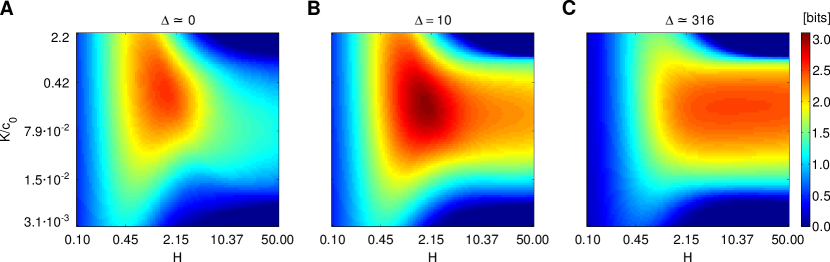
Figure 2: Information planes for different values of the spatial coupling, $\Delta$. Shown is the mutual information $I(x;g)$ as a function of the Hill coefficient $H$ and the activation threshold $K$, (A) with negligible spatial coupling, $\Delta\simeq 0$; (B) with intermediate spatial coupling, $\Delta=10$; and (C) with very strong spatial coupling, $\Delta\simeq 316$. The data shown is for the 1D model with short-correlations assumption.

III.1 Spatial coupling can enhance information transmission

We first assessed how introducing diffusive coupling changes the information capacity of the system in the space of regulatory parameters $K$ and $H$. To establish the baseline for comparison, we started with the case without spatial coupling, $\Delta\simeq 0$, fixing $C=1$ and input gradient length $\lambda=1$. Figure 2A shows the “information plane” for this case, i.e., the mutual information $I(x;g)$ as a function of the Hill coefficient $H$ and the activation threshold $K$. Consistently with our previous studies Tkačik et al. (2008b, 2009), the information plane displays a clear optimal choice of $H$ and $K$ that maximizes information transmission. The optimum results from a nontrivial compromise between evenly spreading the whole dynamic range of the output signal along the $x$-axis, which ideally requires low Hill coefficients and half-activation at the system center ($x=L/2,K=c(L/2)$), and a system-wide minimization of the noise; the latter generally favors activation at high input concentrations (to avoid large fluctuations at low $c$) and thus higher $K$.

Figures 2B and 2C show the same information plane, but now at increasing values for the spatial coupling $\Delta$. The first observation is that with nonzero $\Delta$ information can be increased relative to the baseline at the optimal choice of $H$ and $K$, but that the information drops again when the diffusive coupling is too strong, indicating that there exists a nontrivial optimal value for $\Delta$ that maximizes information. The second observation relates to the concomitant change in the optimal parameters $\{K^{*},H^{*}\}$ as the diffusive coupling is increased. In particular, increasing the diffusion constant shifts the optimum towards higher $H$ and lower $K$. The third observation is that strong diffusion also increases the capacity away from the optimum in the regime of high $H$, creating a flat plateau where the precise value of $H$ is not crucial for attaining high information transmission.

All these observations can be understood intuitively: The increase in capacity for nonzero diffusion is due to the trade-off between the ability of diffusive spatial averaging to reduce noise (thus increasing the transmission), and smoothing out the response profile (thus decreasing the transmission) Erdmann et al. (2009); Sokolowski et al. (2012). The shift in optimal regulatory parameters is a direct consequence of these two effects: the detrimental effect of smoothing out the response profile can be partially compensated for by choosing higher optimal Hill coefficients, while noise reduction allows the optimal $K$ to move towards lower concentrations to better utilize the dynamic range. The plateau in information at high diffusion results from the ability of the diffusion to flatten sharp, nearly step-like gene activation profiles at high $H$ (limited to at most 1 bit of positional information for $H\rightarrow\infty$ and $\Delta\rightarrow 0$) into smooth spatial gradients that can convey more positional information.

III.2 Spatial coupling is most beneficial when input noise is dominant

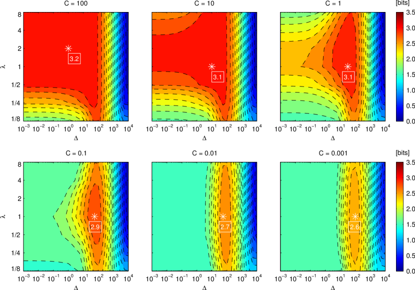
Figure 3: Information transmission as a function of the spatial coupling $\Delta$ and the input gradient length $\lambda$ for various values of maximal input concentration, $C$. For comparison, the same scale is used for all contour maps. White stars mark the overall maximum of $I(x;g)$ in each respective panel; white boxes show the corresponding optimal amount of transmitted information (in bits). Each datapoint was obtained by optimizing $I(x;g)$ over the regulatory parameters $H$ and $K$ for the given set of $C$, $\Delta$ and $\lambda$. The data shown is for the 1D model with short-correlations assumption.

After understanding the optimal behavior of information as a function of regulatory parameters $H,K$ at fixed $C=1$, $\lambda=1$, and $\Delta$, we systematically varied the diffusive coupling $\Delta$ and the input gradient length scale $\lambda$ for several different values of $C$. For each choice of $(\Delta,\lambda)$ parameters, we separately mapped out the information as a function of $H$ and $K$ to find the optimal values $(H^{*},K^{*})$ and the corresponding maximal information transmission.

Figure 3 summarizes this exploration and shows the information capacity as a function of $\Delta$ and $\lambda$ for a series of 6 different $C$ values. White stars mark the maximal capacity for the given $C$, i.e., the capacity for jointly optimal choice of $H$, $K$, $\Delta$ and $\lambda$.

The panel for $C=1$ demonstrates two beneficial effects of diffusion on information capacity: increasing $\Delta$ from very low values to $\Delta\lesssim 100$ increases $I(x;g)$ and simultaneously enlarges the range of $\lambda$ over which high capacity can be reached. This effect is even more pronounced when $C<1$: at very low $C$ the beneficial values for the diffusion constant $\Delta$ are strongly constrained to a narrow interval, and the resulting capacity gain at optimal $\Delta$ with respect to low $\Delta$ increases markedly. In contrast, when $C$ is high, diffusive coupling does not convey a large benefit in information transmission. This is due to the fact that diffusion can only remove super-Poissonian parts of the noise Erdmann et al. (2009); Sokolowski et al. (2012). In our model, super-Poissoninan noise is the input noise, which plays a minor role for $C\gg 1$, thereby limiting the potential role of diffusion. We note that super-Poissonian fluctuations could also occur on the output side (e.g., when gene expression is bursty and multiple protein copies are produced from each mRNA), in which case diffusive coupling could be beneficial even for $C\gg 1$. As expected, for all $C$, the information capacity drops to zero at very high $\Delta$ independently of all other parameters, because in that limit all output profiles become flat and thus uninformative.

Figure 4: Information capacity for varying maximal input concentration, $C$. Shown is the optimized information capacity as a function of $C=c_{\rm max}/c_{0}$ with optimal diffusive coupling ($I^{*}(C)$, solid blue line) and without diffusive coupling ($I_{0}(C)$, dashed blue line). At small $C$, non-Poissonian input noise is dominant, while Poissonian output noise dominates for large $C$. The blue-shaded area depicts the maximal gain in information capacity from diffusive coupling: spatial coupling enhances information capacity most efficiently when input noise dominates. The dashed vertical lines mark the $C$ values corresponding to the three cases displayed in Fig. 5.

We systematically explored how diffusion affects the optimal information transmission as a function of $C$ in Fig. 4, by comparing the optimally coupled spatial model to a model where diffusion is set to zero. Because the information transmission is largely invariant to $\lambda$ and for most values of $C$ peaks in a very broad plateau at $\lambda=1$, we fixed $\lambda=1$ for this comparison, while optimizing over all other parameters (separately for the spatially coupled system and the system with $\Delta\simeq 0$). Clearly, in the low-$C$ regime optimal diffusive coupling can enhance information capacity by more than a bit, while for $C\gtrsim 100$ the noise composition is strongly dominated by Poissonian output noise such that diffusion cannot further improve information throughput.

Instead of varying $C$ by changing the maximal input concentration $c_{\rm max}$, we also varied $C$ via $N_{\rm max}$, thus altering output noise at constant levels of input noise. In that case we observe the same behavior, i.e. significant capacity enhancement by diffusion in the low-$C$ regime, with the small difference that now the capacity increases with decreasing $C\sim 1/N_{\rm max}$, as presented in more detail in Appendix E.

III.3 Spatial coupling enables a novel regulatory strategy at high input noise

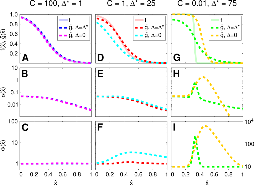
Figure 5: Comparison of optimal output profiles for different values of the maximal input concentration, $C$. (A-C) Dominant output noise, $C=100$, blue lines. (D-F) Balanced noise, $C=1$, red lines. (G-I) Dominant input noise, $C=0.01$, green lines. For every value of $C$, the normalized mean output profile $\bar{g}(\hat{x})$ (dashed lines) and the optimal activation profile $f(\hat{x})$ (faint solid lines) are shown in the top row; the noise in gene expression is shown as the standard deviation $\sigma(\hat{x})$ in the middle row; and the Fano factor $\Phi(\hat{x})=N_{\rm max}\sigma^{2}(\hat{x})/\bar{g}(\hat{x})$, is shown in the bottom row. All profiles are shown as a function of the normalized position, $\hat{x}=x/L$. The corresponding quantities for the optimal spatially uncoupled ($\Delta\simeq 0$) system are shown in complementary colors (see plot legends).

Spatial coupling affects both the noise level of the output gene as well as the shape of its output profile. We wondered how these two effects combine to affect the information transmission. Figure 5 shows the optimal mean output profile $\bar{g}(\hat{x})$, the underlying activation profile $f(\hat{x})$, and two measures of the noise in gene expression, the standard deviation $\sigma^{2}(\hat{x})$ and the Fano factor $\Phi(\hat{x})=N_{\rm max}\hat{\sigma}^{2}(\hat{x})/\bar{g}(\hat{x})$, as a function of position $\hat{x}\equiv x/L\in[0,1]$. We plot these quantities for three values of $C$, representative of the input-noise-dominated regime ($C=0.01$), the regime in which input and output noise are approximately balanced ($C=1$), and the output-noise-dominated regime ($C=100$). In each plot we directly compare the system in which the diffusion constant is optimized along with all other parameters, vs. the system that is optimal at zero spatial coupling.

For $C=100$, input noise levels are so low that the total noise is dominated by purely Poissonian output noise throughout the whole system ($\Phi(\hat{x})\simeq 1$). Therefore, strong spatial coupling would fail to decrease the noise further and would merely fade out the mean output profile. Consequently, the optimal diffusion constant $\Delta^{*}=1$ is low, and the spatially coupled system only differs marginally from the uncoupled system.

For $C=1$ in the uncoupled system, input noise becomes more prominent as a fraction of the total noise, such that $\Phi(\hat{x})>1$ for $\hat{x}\gtrsim 0.3$ (cyan colored line in Fig. 5F); in line with this, the activation threshold is shifted towards higher input concentrations (i.e. smaller $\hat{x}$) at the expense of reducing the dynamic range. In the coupled system the optimal diffusion constant is markedly higher ($\Delta^{*}=25$) than at $C=100$, and the resulting spatial averaging can almost completely remove the additional non-Poissonian noise contributions ($\Phi(\hat{x})\simeq 1$). This allows the optimal activation threshold $K$ to shift towards lower input concentrations in order to attain a similarly large dynamic range as for $C=100$.

At $C=0.01$, when input noise is exceedingly dominant, we observe the emergence of a qualitatively new regulatory strategy in the spatially coupled system. For both spatially coupled and uncoupled systems, low $C$ favors sharp activation profiles with high Hill coefficients $H$. For the spatially uncoupled system, the optimal activation threshold $K^{*}$ moves towards central positions. In contrast, in the optimal spatially coupled system, the optimal activation threshold $K^{*}$ moves closer towards $\hat{x}=0$ where input noise is smaller, and the optimal Hill coefficient makes the activation nearly step-like. Without spatial coupling, this strategy could not be optimal, because it would be limited to at most one bit—in the region where the activation profile is flat, positions could not be discriminated based on the gene expression level $g$. Optimal diffusion can, however, smooth out this step-like activation to generate a graded gene expression profile and restore position discriminability at essentially all positions. Simultaneously, optimal diffusion transforms the noise in an interesting way, as can be seen in Fig. 5H and I. The step-like activation curve suppresses the super-Poissonian input noise everywhere except for the narrow interval of $x$ around the transition point where the super-Poisson component has a very sharp and tall peak; but this can very effectively be removed by the strong diffusive spatial averaging. In sum, at low $C$, the optimal strategy is to use very sharp activation profiles, since they act as a “filter” for input noise (which must go to zero at zero or saturated gene expression); the strong optimal diffusion then smoothes out the step-like activation into a graded response and removes much of the remaining input noise around the very localized transition region at $c\approx K^{*}$.

Usually, the effect of diffusion on information transmission is understood to be a tradeoff between the beneficial effect of noise averaging and detrimental effect of smoothing the profile, but here it seems that smoothing the step-like activation profile is also beneficial for the information flow. To check that this is indeed a qualitatively different optimal regulatory strategy, we performed a systematic study of the optimal regulatory parameters between $C=0.1$ and $C=0.01$. We found that here two regulatory strategies compete, as evidenced by two local maxima in the $(K,H)$ information planes for this range of $C$ values: one favors relatively low Hill coefficients, $H^{*}\simeq 1$, and high activation thresholds $K^{*}$; the other favors high $H^{*}$ and lower $K^{*}$. For $C=0.01$ and $10\lesssim\Delta\lesssim 30$ both regulatory strategies lead to almost equal information capacities, but for $\Delta\gtrsim 30$ steep activation combined with fast diffusion is preferable. Figure S2 in Appendix F illustrates this phenomenon.

III.4 Full solution in 2D geometry differs only marginally from an approximate solution in 1D

All results presented in the previous sections were obtained using the 1D model with short-correlations assumption (SCA). To assess how representative they are of the fully detailed model, we compared the 1D model with SCA to the 2D model with SCA, and finally to the 2D model that retains more than only nearest-neighbor correlations (see Appendix B for the formulas in the first two cases and Appendix C for the latter case).

Figure S3 in Appendix G compares the information planes $I(\Delta,\lambda)$ for the three cases at $C=1$. The results suggest that the influence of lateral spatial coupling present in the 2D model is minor. Particularly in the range of spatial couplings $\Delta$ around the information maximum, where the system is operating close to the hard bound set by irreducible Poissonian noise, the difference between information capacities in 1D and 2D is almost negligible. Inclusion of 2D couplings mainly increases $I(x;g)$ values away from the optimal range of parameters, thus effectively enlarging the region of parameter space in which the system can attain close-to-optimal information transmission. This again is most prominent for the low $C$ regime, as expected, but still limited to a small fraction ($\lesssim 10\%$) of the total capacity (data not shown). The effect of incorporating longer-ranged correlations is minor as well: the information planes for the 2D model with and without SCA are almost indistinguishible.

Overall, this demonstrates that the 1D model with short-correlations assumption is a good approximation of the fully detailed model. In the given context, the strength of spatial coupling appears more relevant than its topology.

IV Discussion

We developed a generic framework to compute information flow through spatially coupled gene regulatory networks at steady state. As the simplest example, we considered how a spatially varying concentration field (“input profile”) is read out collectively by a regular 1D or 2D lattice of sampling units that are interacting by local diffusion of the gene product. A directly applicable example could be cells (or nuclei) in a developing multicellular organism that respond to the morphogen field by expressing developmental genes whose products can be exchanged between neighboring cells. We emphasize that our framework is generic in that effects due to spatial coupling in any chosen geometry can be worked out before assuming any particular gene regulatory function and writing down the relevant noise power spectra, as is evident from Eqs. (9), (10) and (11). This makes the framework widely applicable to a broad range of biological problems in which spatially distributed information is collectively sensed by a set of discrete sampling units and encoded into a spatial output.

The theory presented here is a direct continuation of our previous work on quantifying information flow in gene regulatory networks at increasing levels of realism Tkačik et al. (2008b, 2009); Walczak et al. (2010); Tkačik et al. (2012); Rieckh and Tkačik (2014). In our previous approaches, however, we were striving for analytical approximations that would permit computing the channel capacity, that is, performing analytical optimization over all possible distributions of input signals, $P_{c}(c)$; this led us to adopt the “small noise approximation.” Here, in contrast, we assumed a particular geometry (with a uniform distribution over sampling units, $P_{x}(x)$) and a particular functional form of the input concentration field, $c(x)$; the latter can depend on parameters which one can optimize, but we do not perform functional optimization over all possible $c(x)$. While these restrictions may appear stronger than in our previous work, they also allow us to move to a truly spatially discrete setup (that has a natural minimal spatial scale of a cell or nucleus, as is the case in reality), and permit to relax the small noise approximation, which is no longer assumed in this work. We also note that a parametric choice of $c(x)$ is not as restrictive as it might appear initially. First, one could choose a rich enough parametric form (basis set) for $c(x)$ that ensures spatial smoothness but otherwise allows optimization in a full space of plausible profiles. Second, it is intuitively clear that monotonic functions encode positional information better than non-monotonic, or even constant functions, strongly narrowing the range of functional forms over which optimization should take place. Third, while we focused on exponential gradients which can be easily parametrized by only two parameters, exponential profiles actually are widespread throughout biology Kicheva et al. (2007); Wartlick et al. (2009); Bollenbach et al. (2008); de Lachapelle and Bergmann (2010); Restrepo et al. (2014).

Several previous approaches assessed how diffusive coupling alters the precision of spatial protein patterns driven by spatially distributed inputs Erdmann et al. (2009); Sokolowski et al. (2012); Holloway et al. (2011). While similar in spirit to ours, these works employed measures of “regulatory precision” such as the output pattern steepness and sharpness, which—unlike mutual information—do not capture the problem in its full richness: these measures quantify precision only locally, on parts of the output signal, and moreover, make implicit assumptions about which feature of the output (boundary steepness, boundary position, etc.) is informative. Information theory removes this arbitrariness Tkačik et al. (2015), and permits extensions beyond the simple cases studied here. Similar approaches have recently been suggested for specific biological systems Mugler et al. (2014); Tikhonov et al. (2014); Taillefumier and Wingreen (2014).

In our example application we studied how spatial coupling alters optimal information flow in a single-input/single-output gene regulatory network motivated by the bicoid-hunchback system, which is a part of the gap gene network in early fruit fly development Jaeger (2011); Jaeger et al. (2012). The main outcome of this analysis is that diffusive coupling enhances information capacity by removing super-Poissonian components of the noise, in line with previous work Erdmann et al. (2009); Sokolowski et al. (2012); this effect is large when input noise is non-negligible ($C\leq 1$). When diffusion plays a large role in an optimal system, the activation functions can deviate substantially from the resulting output gene expression profiles. At the extreme, the activation functions can become step-like with very high Hill coefficients, while the gene expression profile still smoothly changes over its full dynamic range; this strategy, optimal at low $C$, where both spatial noise averaging and profile smoothing due to diffusion act jointly to increase information, is qualitatively different from the $C$ regime where profile smoothing is detrimental and trades off against noise averaging.

In our setup, super-Poissoninan contributions to noise are fully accounted for by the input noise, but in reality this need not be the case. There are super-Poissonian contributions to noise that arise at the output, for instance, due to bursty production of proteins when the gene is activated. The simplest case is when mRNA expression is rate limiting, but then each mRNA can lead to a burst in the number of translated proteins. The theory can be simply extended to these cases by introducing a burst size into the relevant noise power spectra. Importantly, this would imply that diffusion can be effective at noise reduction (and thus beneficial for information transmission) also in the regime where $C\geq 1$. In support of this, recently another model linking mRNA expression and protein production with diffusion based on stochastic branching theory has shown that deviations from Poissonian statistics in typical biological conditions are expected only for rather large burst sizes ($\gtrsim 50$) Cottrell et al. (2012).

Recently, the field has made progress in detailed understanding of input-side noise in gene regulation due to stochastic diffusive arrivals of regulatory molecules to their binding sites Kaizu et al. (2014); Paijmans and ten Wolde (2014). This has led to a revision of the previously suggested functional form for the Berg-Purcell limit Berg and Purcell (1977); Bialek and Setayeshgar (2005) that we use in Eq. (13). Furthermore, we have also taken the simplest (Hill-type) regulatory function as our model for gene regulation, rather than picking a richer and potentially more realistic choice, such as the Monod-Wyman-Changeux form. These refinements will be included into our model in the future, but there is no reason to expect that they could change any qualitative outcome of our analyses.

It is interesting to speculate about the predictive power of optimization-based approaches applied to biological systems. In neuroscience, the principle of “efficient coding” which states that neural sensory systems devote their limited resources to maximize the information flow, in bits, from the naturalistic stimuli into the spiking neural representation Tkačik and Bialek (2014), has proven enormously successful since the end of 1950s when it was first suggested by Barlow Barlow (1961). In signaling and gene regulation, similar ideas are much younger. On the other hand, the number of distinct genes or signaling proteins involved in the networks of interest is much smaller than the number of neurons; furthermore, molecular processes and the physical limits to sources of noise in gene regulation might be more easily understood than in neuroscience, where even a single neuron is a very complex object. It appears feasible that for small genetic networks the optimization problem would be tractable upon combining all phenomenology that until now we have analyzed separately: multiple, interacting genes, driven by one or more inputs, potentially with arbitrary feedback, all major relevant sources of noise, spatial coupling, and readout constraints Tkačik et al. (2008b, 2009); Walczak et al. (2010); Tkačik et al. (2012); Rieckh and Tkačik (2014). A major goal would also be the ability to relax the steady-state assumptions, by considering either readout at particular time points (out of steady state), or the information between full state trajectories Tostevin and ten Wolde (2009, 2010); de Ronde et al. (2010); Mugler et al. (2010); Selimkhanov et al. (2014). Such a predictive theory, from which optimal networks could be derived mathematically, could then be realistically confronted with well-studied networks that can be quantitatively measured, e.g., the gap gene network active during Drosophila development Jaeger (2011); Jaeger et al. (2012); Dubuis et al. (2013b). It is intriguing to think that even in the molecular world the need to pay for abstract bits of information—in the currency of time or energy—led nature to choose particular regulatory networks, and perhaps poised them at special operating points Krotov et al. (2014).

V Acknowledgements

The authors thank A. Mugler, I. Nemenman, T. Gregor, M. Tikhonov, P.R. ten Wolde and K. Kaizu for fruitful discussions.

Appendix A Calculation of stationary means and (co)variances

Considering Eq. (2) in steady state immediately yields:

$$\langle F(g_{i},c_{i})\rangle=f(c_{i})-\frac{1}{\tau}\langle g_{i}\rangle$$

$$=h\sum_{n_{i}\in N(i)}\langle g_{i}-g_{n_{i}}\rangle=2dh\langle g_{i}\rangle-h\sum_{n_{i}\in N(i)}\langle g_{n_{i}}\rangle$$

This simply reflects the steady-state balance between production (and degradation) and diffusive in-/outflux in volume $i$. Grouping $\langle g_{i}\rangle$ terms on one side gives

$$\langle g_{i}\rangle =\frac{\tau}{1+2dh\tau}\left(f(c_{i})+h\sum_{n_{i}\in N(i)}\langle g_{n_{i}}\rangle\right)$$

$$\Leftrightarrow\quad\bar{g}_{i} =Tf(c_{i})+\Lambda^{2}\sum_{n_{i}\in N(i)}\bar{g}_{n_{i}}$$ (28)

where in the last step we abbreviate $\bar{g}_{i}\equiv\langle g_{i}\rangle$, $T\equiv\tau/\left(1+2dh\tau\right)$, $\Lambda^{2}\equiv hT$, as in the main text.

To simplify the steady-state expression for the covariances resulting from Eq. (3) it is instructive to treat its different parts separately. For the terms correlating the fluctuations in volume $i$ with the production/degradation process in volume $j$ we have (note that $\langle\delta g_{i}\rangle=0$ by construction):

$$\langle\delta g_{i}F(g_{j},c_{j})\rangle =\langle\delta g_{i}\rangle f(c_{j})-\frac{1}{\tau}\langle\delta g_{i}g_{j}\rangle$$

$$=-\frac{1}{\tau}\langle\delta g_{i}\left(\langle g_{j}\rangle+\delta g_{j}\right)\rangle=-\frac{1}{\tau}\langle\delta g_{i}\delta g_{j}\rangle$$ (29)

Hence,

$$\langle\delta g_{i}F(g_{j},c_{j})\rangle+\langle\delta g_{j}F(g_{i},c_{i})\rangle=-\frac{2}{\tau}\langle\delta g_{i}\delta g_{j}\rangle$$ (30)

because $\langle\delta g_{i}\delta g_{j}\rangle\equiv\langle\delta g_{j}\delta g_{i}\rangle$.

Similarly, we can rewrite the term that correlates $\delta g_{i}$ with the diffusive “neighbor fluxes” of $g_{j}$

$$h\left\langle\delta g_{i}\sum_{n_{j}\in N(j)}(g_{n_{j}}-g_{j})\right\rangle$$

$$=h\left\langle\delta g_{i}\sum_{n_{j}\in N(j)}\left(\langle g_{n_{j}}\rangle+\delta g_{n_{j}}-\langle g_{j}\rangle-\delta g_{j}\right)\right\rangle$$

$$=h\left(\sum_{n_{j}\in N(j)}\langle\delta g_{i}\rangle\langle g_{n_{j}}\rangle+\langle\delta g_{i}\delta g_{n_{j}}\rangle\right)$$

$$\qquad\qquad\qquad\qquad\qquad-2dh\left(\langle\delta g_{i}\rangle\langle g_{j}\rangle-\langle\delta g_{i}\delta g_{j}\rangle\right)$$

$$=h\left(\sum_{n_{j}\in N(j)}\langle\delta g_{i}\delta g_{n_{j}}\rangle\right)-2dh\langle\delta g_{i}\delta g_{j}\rangle$$ (31)

and analogously for the term in which $i$ and $j$ are exchanged.

Reinserting (30) and (31) into the right side of Eq. (3), collecting covariance terms $\langle\delta g_{i}\delta g_{j}\rangle$ on the left side, and multiplying by $\tau/2$ we obtain:

$$\left(1+2dh\tau\right)\langle\delta g_{i}\delta g_{j}\rangle$$

$$=\frac{h\tau}{2}\left(\sum_{n_{j}\in N(j)}\langle\delta g_{i}\delta g_{n_{j}}\rangle+\sum_{n_{i}\in N(i)}\langle\delta g_{j}\delta g_{n_{i}}\rangle\right)$$

$$\qquad\qquad\qquad\qquad\qquad\qquad\quad+\frac{\tau}{2}\sum_{k}\left\langle\Gamma_{ik}\Gamma_{jk}\right\rangle$$

$$\Leftrightarrow\quad C_{ij}=\frac{\Lambda^{2}}{2}\left(\sum_{n_{j}\in N(j)}C_{in_{j}}+\sum_{n_{i}\in N(i)}C_{jn_{i}}\right)$$

$$\qquad\qquad\qquad\qquad\qquad\qquad\quad+\frac{T}{2}\sum_{k}\left\langle\Gamma_{ik}\Gamma_{jk}\right\rangle$$ (32)

where $C_{ij}\equiv\langle\delta g_{i}\delta g_{j}\rangle$. The above equation couples the covariance $C_{ij}$ to the covariances $C_{in_{j}}$ and $C_{jn_{i}}$; these represent the correlations between the protein number in volume $i$ and the neighbor volumes $n_{j}$ of $j$, and the analogous quantity with $i$ and $j$ exchanged, respectively. Hence, even if $i$ and $j$ are nearest neighbors on the lattice, the expressions summing $C_{in_{j}}$ and $C_{jn_{i}}$ over $n_{j}$ and $n_{i}$, respectively, will contain correlations between next-nearest neighbor volumes. While the equation system defined by Eq. (32) can be solved for the whole set of covariances $C_{ij}$ upon imposing suitable boundary conditions, this can be numerically expensive for larger spatial lattices and large parameter sweeps as part of optimization runs. In this work, the quantity of interest is the variance $C_{ii}$ in volume $i$, such that the calculation of longer-ranged correlations is not strictly required.

Considering the cases $i=j$ and $\nu\in N(i)$ ($\nu$ being one of the nearest neighbors of $i$) in Eq. (32) separately reveals the following interdependence between the variance $\sigma^{2}_{i}\equiv C_{ii}$ and the nearest-neighbor covariance $C_{i\nu}$:

$$\sigma^{2}_{i} =\Lambda^{2}\sum_{\nu\in N(i)}C_{i\nu}+\frac{T}{2}\sum_{k}\left\langle\Gamma_{ik}^{2}\right\rangle$$ (33)

$$C_{i\nu} =\frac{\Lambda^{2}}{2}\left(\sum_{n_{\nu}\in N(\nu)}C_{in_{\nu}}+\sum_{n_{i}\in N(i)}C_{\nu n_{i}}\right)$$

$$\qquad\qquad\qquad\qquad\qquad+\frac{T}{2}\sum_{k}\left\langle\Gamma_{ik}\Gamma_{\nu k}\right\rangle$$ (34)

Next-nearest correlations now only appear in Eq. (34), which can be significantly simplified by an approximation that we call the “short-correlations assumption” (SCA): If the next-nearest-neighbor covariances are assumed to be small compared to the nearest-neighbor covariances and single-point variances, we can ignore them and set

$$C_{in_{\nu}}=0\qquad\forall n_{\nu}\neq i$$

$$C_{\nu n_{i}}=0\qquad\forall n_{i}\neq\nu$$ (35)

because then the only neighbor of $\nu$ that has some significant correlation with $i$ is $i$ itself, and vice versa. In that case, the only remaining terms of the sums in Eq. (34) are $C_{ii}=\sigma^{2}_{i}$ and $C_{\nu\nu}=\sigma^{2}_{\nu}$, respectively:

$$C_{i\nu} =\frac{\Lambda^{2}}{2}\left(\sigma^{2}_{ii}+\sigma^{2}_{\nu\nu}\right)+\frac{T}{2}\sum_{k}\left\langle\Gamma_{ik}\Gamma_{\nu k}\right\rangle$$ (36)

Specifying further the noise powers $\sum_{k}\left\langle\Gamma_{ik}^{2}\right\rangle$ in (33) and $\sum_{k}\left\langle\Gamma_{ik}\Gamma_{\nu k}\right\rangle$ in (36) as described in Section II.2 yields formulas (10) and (11).

Appendix B Simplified variance formulae

In our framework, computation of the mutual information $I(x;g)$ only requires the means $\bar{g}_{i}$ and variances $\sigma^{2}_{i}$. This enables us to reduce the number of coupled equations to be solved by direct insertion of (11) into (10), thus eliminating $C_{ij}$. For the 1D model with short-correlations assumption (SCA), after some algebraic steps this yields

$$\sigma^{2}_{i} =\frac{\Delta^{2}}{\left(1+2\Delta\right)^{2}-\Delta^{2}}\frac{1}{2}\left(\sigma^{2}_{i-1}+\sigma^{2}_{i-1}\right)$$

$$\quad+\frac{1}{N_{\rm max}}\bBigg@{3}\{\frac{1+2\Delta}{\left(1+2\Delta\right)^{2}-\Delta^{2}}\times$$

$$\qquad\qquad\qquad\quad\left(\frac{f(c_{i})+\bar{g}_{i}}{2}+\left[\left(\frac{\partial f}{\partial c}\right)^{2}cc_{0}\right]_{c_{i}}\right)$$

$$\qquad+\frac{\Delta}{\left(1+2\Delta\right)+\Delta}\frac{1}{2}\left(\bar{g}_{i-1}+2\bar{g}_{i}+\bar{g}_{i+1}\right)\bBigg@{3}\}$$ (37)

where we have rewritten prefactor combinations containing $T$ and $\Lambda^{2}$ in terms of the spatial coupling $\Delta$.

The analogous formula for the 2D model with SCA reads

$$\sigma^{2}_{(ij)} =\frac{\Delta^{2}}{\left(1+4\Delta\right)^{2}-2\Delta^{2}}\frac{1}{2}\sum_{n_{(ij)}}\sigma^{2}_{n_{(ij)}}$$

$$\quad+\frac{1}{N_{\rm max}}\bBigg@{3}\{\frac{1+4\Delta}{\left(1+4\Delta\right)^{2}-2\Delta^{2}}$$

$$\qquad\qquad\quad\times\left(\frac{f(c_{(ij)})+\bar{g}_{(ij)}}{2}+\left[\left(\frac{\partial f}{\partial c}\right)^{2}cc_{0}\right]_{c_{(ij)}}\right)$$

$$\qquad+\frac{\Delta\left(1+3\Delta\right)}{\left(1+4\Delta\right)^{2}-2\Delta^{2}}\frac{1}{2}\left[4\bar{g}_{(ij)}+\sum_{n_{(ij)}}\bar{g}_{n_{(ij)}}\right]\bBigg@{3}\}$$

where we indicate volumes of the two-dimensional lattice with a 2D index $(ij)$, and the $n_{(ij)}$-sums run over the four nearest neighbor volumes of $(ij)$.

Appendix C Full solution without short-correlations assumption

For completeness, here we also state the formula defining the linear system for the coupled covariances in the full two-dimensional model without short-correlations assumption, again indicating volumes by the two-dimensional index $(ij)$:

$$C_{(ij)(kl)} =\frac{1}{2}\frac{1}{1+4\Delta}\Bigg{\{}\hat{\mathcal{N}}^{2}_{(ij)(kl)}$$

$$\qquad\qquad+\Delta\Big{[}\quad C_{(ij)(k-1,l)}+C_{(ij)(k+1,l)}$$

$$\phantom{\qquad\qquad\Delta\Big{[}\quad}+C_{(ij)(k,l-1)}+C_{(ij)(k,l+1)}$$

$$\phantom{\qquad\qquad\Delta\Big{[}\quad}+C_{(i-1,j)(kl)}+C_{(i+1,j)(kl)}$$

$$\phantom{\qquad\qquad\Delta\Big{[}\quad}+C_{(i,j-1)(kl)}+C_{(i,j+1)(kl)}\Big{]}\Bigg{\}}$$

where the normalized noise term $\hat{\mathcal{N}}^{2}_{(ij)(kl)}$ is only non-zero if the volumes indicated by $(ij)$ and $(kl)$ are identical, i.e. $(ij)\equiv(kl)$, or nearest neighbors, i.e. $(kl)\in N((ij))$, and takes one of the following forms, respectively:

$$\hat{\mathcal{N}}^{2}_{(ij)(kl)}=\hat{\mathcal{N}}^{2}_{(ij)(ij)}$$

$$=\hat{\mathcal{G}}^{2}_{(ij)}+\sum_{n_{(ij)}}\left(\hat{\mathcal{D}}^{2}_{[(ij)\rightarrow n_{(ij)}]}+\hat{\mathcal{D}}^{2}_{[n_{(ij)}\rightarrow(ij)]}\right)$$

$$\text{if }(ij)\equiv(kl)$$

$$\hat{\mathcal{N}}^{2}_{(ij)(kl)}=-\left(\hat{\mathcal{D}}^{2}_{[(ij)\rightarrow(kl)]}+\hat{\mathcal{D}}^{2}_{[(kl)\rightarrow(ij)]}\right)$$

$$\text{if }(kl)\in N((ij))$$

$$\hat{\mathcal{N}}^{2}_{(ij)(kl)}\equiv 0\qquad\qquad\qquad\qquad\,\text{else}$$ (40)

Here $n_{(ij)}$ runs over the four nearest-neighbors of volume $(ij)$. The normalized noise powers $\hat{\mathcal{G}}^{2}_{(ij)}$ and $\hat{\mathcal{D}}^{2}_{[(ij)\rightarrow(kl)]}$ derive from the expressions presented in Section II.3:

$$\hat{\mathcal{G}}^{2}_{(ij)}=\frac{1}{N_{\rm max}}\left(f(c_{(ij)})+\bar{g}_{(ij)}+\left[\left(\frac{\partial f}{\partial c}\right)^{2}2cc_{0}\right]_{c_{(ij)}}\right)$$

$$\hat{\mathcal{D}}^{2}_{[(ij)\rightarrow(kl)]}=\frac{\Delta}{N_{\rm max}}\bar{g}_{(ij)}$$ (41)

Eq. (LABEL:eqCovariancesNoSCA) in principle allows for calculation of covariances between volumes that are arbitrarily far apart. In practice, because of the finiteness of the lattice, the spatial correlations still have to be truncated at a certain distance and boundary conditions applied in order to obtain a closed system that consists of as many equations as variables.

Appendix D Standard parameters

Quantity	Symbol	Value
Lattice spacing	$\delta$	8.33 $\mu m$
No. of nuclei in $x$-direction	$N_{x}$	60
– resulting system length	$L$	500 $\mu m$
Internal activator diffusion constant	$D_{c}$	3.16 $\mu m^{2}/s$
Activator binding site length	$l_{c}$	0.01 $\mu m$
Product protein lifetime	$\tau$	240 $s$
Std. max. mean product copy no.	$N_{\rm max}^{0}$	444
– resulting typ. concentration	$c_{0}$	58.5 $\mu m^{-3}$
		($\simeq 35~{}nM$)
– resulting typ. diffusion constant	$D_{0}$	0.29 $\mu m^{2}/s$
Std. input gradient length	$\gamma_{0}$	100 $\mu m$
Std. input gradient amplitude	$c_{\rm max}$	$=c_{0}$

Table 1: The standard parameter values of our model.

In our derivations most system parameters can be combined into two natural scales, a typical concentration $c_{0}$ (cf. Section II.3) and a typical diffusion constant $D_{0}$ (cf. Section II.2), and we measure concentrations and diffusion in these scales throughout our theory. To obtain numerical solutions, however, concrete numbers have to be assigned to these quantities.

Since our example application represents the bicoid-hunchback system in early Drosophila development, we opted for the following choice for the baseline values of the parameters in Table 1: First we chose lattice parameters that roughly correspond to the geometry of the Drosophila syncytium Gregor et al. (2007a, b); in particular, this defines the lattice spacing $\delta$. We then chose a typical value for the product protein lifetime $\tau$, which defines the typical diffusion scale $D_{0}=\delta^{2}/\tau$.

To set the value for $c_{0}$, we took advantage of the fact that in the bicoid-hunchback system the activator (i.e. Bicoid) concentration at midembryo has been measured experimentally Houchmandzadeh et al. (2002); Gregor et al. (2007a). This lead us to set $c_{0}$ equal to the extrapolated maximal value of the measured in-vivo gradient at its source ($x=0$). In other words, at $C=c_{\rm max}/c_{0}=1$ the input function $c(x)$ in our model corresponds to the experimentally measured Bicoid gradient. Finally, to define a standard value for the maximal mean output $N_{\rm max}$, which is a key determinant of the noise powers and variances (cf. Eqs. (18), (19), (37), (LABEL:eqVarianceSimplified2D) and (41)) but to-date unknown, we chose typical values for the internal activator diffusion constant $D_{c}$ and the binding site length $l_{c}$; from this, we calculated the standard value $N_{\rm max}^{0}=c_{0}D_{c}l_{c}\tau$. When varying $C$ away from the baseline setting, we changed either $c_{\rm max}$ while holding $N_{\rm max}$ (and thus $c_{0}$) constant, or by varying $N_{\rm max}$ and keeping $c_{\rm max}$ unchanged, as described in Appendix E.

Table 1 demonstrates that all baseline parameter values are well within a biologically realistic regime.

Appendix E Varying $C$ via $N_{\rm max}$

Figure S1: Information capacity for varying noise type ratios, varied via $N_{\rm max}$. Shown is the optimized information capacity as a function of the noise type ratio $C=c_{\rm max}/c_{0}$ with optimal diffusive coupling ($I^{*}(C)$, solid blue line) and without diffusive coupling ($I_{0}(C)$, dashed blue line). $C$ was varied via $N_{\rm max}$. At small $C$ values, non-Poissonian input noise is dominant, while Poissonian output noise dominates for large $C$. The blue-shaded area depicts the maximal gain in information capacity from diffusive coupling.

In our model, the noise type ratio $C=c_{\rm max}/c_{0}=c_{\rm max}/N_{\rm max}\cdot(D_{c}l_{c}\tau)$ can be varied in multiple ways. In addition to altering the importance of non-Poissonian input noise via $c_{\rm max}$, we also studied the case in which the contribution of Poissonian output noise is varied via $N_{\rm max}$ while $c_{\rm max}$ is held constant.

The main difference to the case in which $c_{\rm max}$ is scaled is that now information capacities decrease with increasing $C$, as this means decreasing $N_{\rm max}$ and thus enhancing output noise. The highest information capacity then is attained in the limit $C\rightarrow 0$, i.e. $N_{\rm max}\rightarrow\infty$. In the uncoupled system, $I(x;g)$ saturates for $C\rightarrow 0$ towards a value dictated by the amount of (in this case) irreducible input noise, set by $c_{\rm max}$. With spatial coupling, optimal $I(x;g)$ values in the low-$C$ regime are markedly higher, in accordance with the finding that spatial averaging can only enhance information capacity when input noise is dominant. As expected, for $C\rightarrow 0$, i.e. negligible output noise, and sufficiently strong spatial coupling, i.e. strongly attenuated input noise, the capacity approaches the hard bound of the noise-free limit given by the finite number of sampling points $N_{x}$ along the $x$-axis, $I_{N_{x}}^{\rm max}=\log_{2}(N_{x})$.

Appendix F Double maximum

In Fig. S2 we show three different information planes for noise-type ratio $C=0.01$ and increasing values of the spatial coupling $\Delta$ ($\Delta=1$, $\Delta=10$ and $\Delta=100$). The heat maps demonstrate the emergence of distinct optimal regulatory strategies for $\Delta>1$: for sufficiently strong diffusion ($\Delta=10$), very steep activation curves ($H\gg 1$) at lower activation thresholds $K$ result in similar information transmission as less steep activation curves ($H\simeq 1$) at slightly higher $K$. For $\Delta=100$, steep activation performs better than the other strategy. This effect is seen most clearly in the 2D model (with SCA), but also appears in the 1D model at slightly different values of $C$ and $\Delta$.

Figure S2: Emergence of a second maximum in the information plane. Here we plot for $C=0.01$ and standard input gradient length, i.e. $\lambda=1$, the the positional information $I(x;g)$ as a function of the regulatory parameters $H$ and $K$ for increasing strength of spatial coupling: (A) $\Delta=1$, (B) $\Delta=10$, and (C) $\Delta=100$. White stars mark local maxima, white boxes show the corresponding amount of information in bits. The data shown is for the 2D model with SCA.

Appendix G Model comparison

Figure S3: Comparison of $I(x;g)$ for increasingly detailed versions of the spatial-stochastic model at $C=1$. The reference plot for the 1D model with SCA (left) is identical to the information plane for $C=1$ in Fig. 3. The same information plane is shown for the 2D model with SCA (middle), and for the full 2D model that retains next-nearest neighbor correlations (right).

In Fig. S3 we demonstrate how including increasing detail affects our results for a paradigmatic case ($C=1$, $\lambda=1$). The different panels show the same information plane for the 1D model with SCA, the 2D model with SCA and the 2D model without SCA, which retains longer-ranged correlations with next-nearest neighbor volumes.

References

- van Kampen (1981) N. G. van Kampen, Stochastic processes in physics and chemistry (North Holland, Amsterdam, 1981).
- Tsimring (2014) L. S. Tsimring, Rep Prog Phys 77, 026601 (2014).
- Lo et al. (2015) W.-C. Lo, S. Zhou, F. Y.-M. Wan, A. D. Lander, and Q. Nie, J R Soc Interface 12, 20141041 (2015).
- Zhang et al. (2012) L. Zhang, K. Radtke, L. Zheng, A. Q. Cai, T. F. Schilling, and Q. Nie, Mol Syst Biol 8, 613 (2012).
- Eldar et al. (2004) A. Eldar, B.-Z. Shilo, and N. Barkai, Curr Op Gen Dev 14, 435 (2004).
- Eldar et al. (2002) A. Eldar, R. Dorfman, D. Weiss, H. Ashe, B.-Z. Shilo, and N. Barkai, Nature 419, 304 (2002).
- Tkačik and Walczak (2011) G. Tkačik and A. M. Walczak, J Phys Condens Matter 23, 153102 (2011).
- Tkačik et al. (2008a) G. Tkačik, C. G. Callan, and W. Bialek, Proc Natl Acad Sci USA 105, 12265 (2008a).
- Dubuis et al. (2013a) J. O. Dubuis, G. Tkačik, E. F. Wieschaus, T. Gregor, and W. Bialek, Proc Natl Acad Sci USA 110, 16301 (2013a).
- Tkačik et al. (2008b) G. Tkačik, C. G. Callan, and W. Bialek, Phys Rev E 78, 011910 (2008b).
- Tkačik et al. (2009) G. Tkačik, A. M. Walczak, and W. Bialek, Phys Rev E 80, 031920 (2009).
- Walczak et al. (2010) A. M. Walczak, G. Tkačik, and W. Bialek, Phys Rev E 81, 041905 (2010).
- Tkačik et al. (2012) G. Tkačik, A. M. Walczak, and W. Bialek, Phys Rev E 85, 041903 (2012).
- Rieckh and Tkačik (2014) G. Rieckh and G. Tkačik, Biophys J 106, 1194 (2014).
- Tostevin and ten Wolde (2009) F. Tostevin and P. R. ten Wolde, Phys Rev Lett 102, 218101 (2009).
- Tostevin and ten Wolde (2010) F. Tostevin and P. R. ten Wolde, Phys Rev E 81, 061917 (2010).
- de Ronde et al. (2010) W. H. de Ronde, F. Tostevin, and P. R. ten Wolde, Phys Rev E 82, 031914 (2010).
- Mugler et al. (2010) A. Mugler, A. M. Walczak, and C. H. Wiggins, Phys Rev Lett 105, 058101 (2010).
- Selimkhanov et al. (2014) J. Selimkhanov, B. Taylor, J. Yao, A. Pilko, J. Albeck, A. Hoffmann, L. Tsimring, and R. Wollman, Science 346, 1370 (2014).
- Jaeger (2011) J. Jaeger, Cell Mol Life Sci 68, 243 (2011).
- Jaeger et al. (2012) J. Jaeger, Manu, and J. Reinitz, Curr Op Gen Dev 22, 533 (2012).
- Rushlow and Shvartsman (2012) C. A. Rushlow and S. Y. Shvartsman, Curr Op Genetics of system biology, 22, 542 (2012).
- Restrepo et al. (2014) S. Restrepo, J. Zartman, and K. Basler, Curr Biol 24, R245 (2014).
- Wartlick et al. (2009) O. Wartlick, A. Kicheva, and M. González-Gaitán, Cold Spring Harb Perspect Biol 1, a001255 (2009).
- Meinhardt (1982) H. Meinhardt, Models of Biological Pattern Formation (Academic Press, London, 1982).
- Gregor et al. (2010) T. Gregor, K. Fujimoto, N. Masaki, and S. Sawai, Science 328, 1021 (2010).
- Kamino et al. (2011) K. Kamino, K. Fujimoto, and S. Sawai, Dev Growth Differ 53, 503 (2011).
- Sun et al. (2012) B. Sun, J. Lembong, V. Normand, M. Rogers, and H. A. Stone, Proc Natl Acad Sci USA 109, 7753 (2012).
- Sun et al. (2013) B. Sun, G. Duclos, and H. Stone, Phys Rev Lett 110, 158103 (2013).
- Erdmann et al. (2009) T. Erdmann, M. Howard, and P. R. ten Wolde, Phys Rev Lett 103, 258101 (2009).
- Sokolowski et al. (2012) T. R. Sokolowski, T. Erdmann, and P. R. ten Wolde, PLoS Comput Biol 8, e1002654 (2012).
- Little et al. (2013) S. C. Little, M. Tikhonov, and T. Gregor, Cell 154, 789 (2013).
- Garcia et al. (2013) H. Garcia, M. Tikhonov, A. Lin, and T. Gregor, Curr Biol 23, 2140 (2013).
- Mugler et al. (2014) A. Mugler, M. D. Brennan, A. Levchenko, and I. Nemenman (talk at 8th q-bio Conference, Sante Fe, New Mexico, USA, and personal communication, 2014).
- Tikhonov et al. (2014) M. Tikhonov, S. C. Little, T. Gregor, and W. Bialek (talk at 8th q-bio Conference, Sante Fe, New Mexico, USA, and personal communication, 2014).
- Houchmandzadeh et al. (2002) B. Houchmandzadeh, E. Wieschaus, and S. Leibler, Nature 415, 798 (2002).
- Gregor et al. (2007a) T. Gregor, E. F. Wieschaus, A. P. McGregor, W. Bialek, and D. W. Tank, Cell 130, 141 (2007a).
- Gregor et al. (2007b) T. Gregor, D. W. Tank, E. F. Wieschaus, and W. Bialek, Cell 130, 153 (2007b).
- Dubuis et al. (2013b) J. O. Dubuis, R. Samanta, and T. Gregor, Mol Syst Biol 9, 639 (2013b).
- Petkova et al. (2014) M. D. Petkova, S. C. Little, F. Liu, and T. Gregor, Current Biology 24, 1283 (2014).
- Manu et al. (2009) Manu, S. Surkova, A. V. Spirov, V. V. Gursky, H. Janssens, A.-R. Kim, O. Radulescu, C. E. Vanario-Alonso, D. H. Sharp, M. Samsonova, and J. Reinitz, PLoS Biol 7, 591 (2009).
- de Lachapelle and Bergmann (2010) A. M. de Lachapelle and S. Bergmann, Mol S 6, 351 (2010).
- Wolpert (1969) L. Wolpert, J Theor Biol 25, 1 (1969).
- Wolpert (1994) L. Wolpert, Dev Genet 15, 485 (1994).
- Wolpert (1996) L. Wolpert, Trends in Genetics 12, 359 (1996).
- Wolpert (2011) L. Wolpert, J Theor Biol 269, 359 (2011).
- Hironaka and Morishita (2012) K. Hironaka and Y. Morishita, Curr Op Gen Dev 22, 553 (2012).
- Tkačik et al. (2015) G. Tkačik, J. O. Dubuis, M. D. Petkova, and T. Gregor, Genetics 199, 39 (2015).
- Hasegawa (2006) H. Hasegawa, J Phys Soc Jpn 75, 033001 (2006), arXiv:cond-mat/0512429.
- Hasegawa (2007) H. Hasegawa, Physica A 374, 585 (2007).
- Rodriguez and Tuckwell (1996) R. Rodriguez and H. C. Tuckwell, Phys Rev E 54, 5585 (1996).
- Gillespie (2000) D. T. Gillespie, J Chem Phys 113, 297 (2000).
- Hattne et al. (2005) J. Hattne, D. Fange, and J. Elf, Bioinformatics 21, 2923 (2005).
- Elf and Ehrenberg (2004) J. Elf and M. Ehrenberg, Syst Biol (Stevenage) 1, 230 (2004), PMID: 17051695.
- Tkačik et al. (2008c) G. Tkačik, T. Gregor, and W. Bialek, PLoS ONE 3, e2774 (2008c).
- Tkačik and Bialek (2009) G. Tkačik and W. Bialek, Physical Review E 79, 051901 (2009).
- Shannon (1948) C. E. Shannon, Bell Sys Tech J 27, 379 (1948).
- Kolmogorov (1965) A. Kolmogorov, Problemy Peredachi Informatsii 1, 3 (1965).
- Bollenbach et al. (2008) T. Bollenbach, P. Pantazis, A. Kicheva, C. Bökel, M. González-Gaitán, and F. Jülicher, Development 135, 1137 (2008).
- Kicheva et al. (2007) A. Kicheva, P. Pantazis, T. Bollenbach, Y. Kalaidzidis, T. Bittig, F. Jülicher, and M. González-Gaitán, Science 315, 521 (2007).
- Holloway et al. (2011) D. M. Holloway, F. J. P. Lopes, L. da Fontoura Costa, B. A. N. Travençolo, N. Golyandina, K. Usevich, and A. V. Spirov, PLoS Comput Biol 7, e1001069 (2011).
- Taillefumier and Wingreen (2014) T. Taillefumier and N. S. Wingreen, arXiv:1412.7767 [physics, q-bio] (2014).
- Cottrell et al. (2012) D. Cottrell, P. S. Swain, and P. F. Tupper, Proc Natl Acad Sci USA 109, 9699 (2012).
- Kaizu et al. (2014) K. Kaizu, W. de Ronde, J. Paijmans, K. Takahashi, F. Tostevin, and P. R. ten Wolde, Biophys J 106, 976 (2014).
- Paijmans and ten Wolde (2014) J. Paijmans and P. R. ten Wolde, Phys Rev E 90, 032708 (2014).
- Berg and Purcell (1977) H. C. Berg and E. M. Purcell, Biophys J 20, 193 (1977).
- Bialek and Setayeshgar (2005) W. Bialek and S. Setayeshgar, Proc Natl Acad Sci USA 102, 10040 (2005).
- Tkačik and Bialek (2014) G. Tkačik and W. Bialek, arXiv:1412.8752 [cond-mat, physics:physics, q-bio] (2014).
- Barlow (1961) H. B. Barlow, in Sensory Communication, edited by W. A. Rosenbluth (MIT, Cambridge, MA, USA, 1961) pp. 217–234.
- Krotov et al. (2014) D. Krotov, J. O. Dubuis, T. Gregor, and W. Bialek, Proc Natl Acad Sci USA , 201324186 (2014).