Boundary value problems for Willmore curves in $\mathbb{R}^{2}$

Abstract.

In this paper the Navier problem and the Dirichlet problem for Willmore curves in $\mathbb{R}^{2}$ is solved.

1. Introduction

The Willmore functional of a given smooth regular curve $\gamma\in C^{\infty}([0,1],\mathbb{R}^{n})$ is given by

$$W(\gamma):=\frac{1}{2}\int_{\gamma}\kappa_{\gamma}^{2}$$

where $\kappa_{\gamma}$ denotes the signed curvature function of $\gamma$. The value $W(\gamma)$ can be interpreted as a bending energy of the curve $\gamma$ which one usually tends to minimize in a suitable class of admissible curves where the latter is chosen according to the mathematical or real-world problem one is interested in. One motivation for considering boundary value problems for Willmore curves originates from the industrial fabrication process called wire bonding [4]. Here, engineers aim at interconnecting small semiconductor devices via wire bonds in such a way that energy losses within the wire are smallest possible. Typically the initial position and direction as well as the end position and direction of the curve are prescribed by the arrangement of the semiconductor devices. Neglecting energy losses due to the length of a wire one ends up with studying the Dirichlet problem for Willmore curves in $\mathbb{R}^{3}$. In the easier two-dimensional case the Dirichlet problem consists of finding a regular curve $\gamma\in C^{\infty}([0,1],\mathbb{R}^{2})$ satisfying

(1) $$W^{\prime}(\gamma)=0,\qquad\gamma(0)=A,\;\gamma(1)=B,\qquad\frac{\gamma^{\prime}(0)}{\|\gamma^{\prime}(0)\|}=\begin{pmatrix}\cos(\theta_{1})\\ \sin(\theta_{1})\\ \end{pmatrix},\;\frac{\gamma^{\prime}(1)}{\|\gamma^{\prime}(1)\|}=\begin{pmatrix}\cos(\theta_{2})\\ \sin(\theta_{2})\\ \end{pmatrix}$$

for given boundary data $A,B\in\mathbb{R}^{2}$ and $\theta_{1},\theta_{2}\in\mathbb{R}$. Here we used the shorthand notation $W^{\prime}(\gamma)=0$ in order to indicate that $\gamma$ is a Willmore curve which, by definition, is a critical point of the Willmore functional. Our main result, however, concerns the Navier problem for Willmore curves in $\mathbb{R}^{2}$ where one looks for regular curves $\gamma\in C^{\infty}([0,1],\mathbb{R}^{2})$ satisfying

(2) $$W^{\prime}(\gamma)=0,\qquad\gamma(0)=A,\;\gamma(1)=B,\qquad\kappa_{\gamma}(0)=\kappa_{1},\;\kappa_{\gamma}(1)=\kappa_{2}$$

for given $A,B\in\mathbb{R}^{2}$ and $\kappa_{1},\kappa_{2}\in\mathbb{R}$. In the special case $\kappa_{1}=\kappa_{2}=:\kappa$ the boundary value problem (2) was investigated by Deckelnick and Grunau [2] under the restrictive assumption that $\gamma$ is a smooth symmetric graph lying on one side of the straight line joining $A$ and $B$. More precisely they assumed $A=(0,0),B=(1,0)$ as well as $\gamma(t)=(t,u(t))\,(t\in[0,1])$ for some positive symmetric function $u\in C^{4}(0,1)\cap C^{2}[0,1]$. They found that there is a positive number $M_{0}\approx 1.34380$ such that (2) has precisely two graph solutions for $0<|\kappa|<M_{0}$, precisely one graph solution for $|\kappa|\in\{0,M_{0}\}$ and no graph solutions otherwise, see Theorem 1 in [2]. In a subsequent paper [3] the same authors proved stability and symmetry results for such Willmore graphs. Up to the author’s knowledge no further results related to the Navier problem are known. The aim of our paper is to fill this gap in the literature by providing the complete solution theory both for the Navier problem and for the Dirichlet problem. Special attention will be paid to the symmetric Navier problem

(3) $$W^{\prime}(\gamma)=0,\qquad\gamma(0)=A,\;\gamma(1)=B,\qquad\kappa_{\gamma}(0)=\kappa,\;\kappa_{\gamma}(1)=\kappa$$

which, as we will show in Theorem 1, admits a beautiful solution theory extending the results obtained in [2] which we described above. Our results concerning this boundary value problem not only address existence and multiplicity issues but also qualitative information about the solutions are obtained. In [2] the authors asked whether symmetric boundary conditions imply the symmetry of the solution. In order to analyse such interesting questions not only for Willmore graphs as in [2, 3] but also for general Willmore curves we fix the notions of axially symmetric respectively pointwise symmetric regular curves which we believe to be natural.

Definition 1.

Let $\gamma\in C^{\infty}([0,1],\mathbb{R}^{2})$ be a regular curve of length $L>0$ and let $\hat{\gamma}$ denote its arc-length parametrization. Then $\gamma$ is said to be

• axially symmetric if there is an orthogonal matrix $P\in O(2)$ satisfying $\det(P)=-1$ such that $s\mapsto\hat{\gamma}(s)+P\hat{\gamma}(L-s)$ is constant on $[0,L]$,

• pointwise symmetric if $s\mapsto\hat{\gamma}(s)+\hat{\gamma}(L-s)$ is constant on $[0,L]$.

Let us shortly explain why these definitions are properly chosen. First, being axially or pointwise symmetric does not depend on the parametrization of the curve, which is a necessary condition for a geometrical property. Second, the definition from (i) implies $P(\hat{\gamma}(L)-\hat{\gamma}(0))=\hat{\gamma}(L)-\hat{\gamma}(0)$ so that $P$ realizes a reflection about the straight line from $\gamma(0)=\hat{\gamma}(0)$ to $\gamma(1)=\hat{\gamma}(L)$. Hence, (i) may be considered as a natural generalization of the notion of a symmetric function. Similarly, (ii) extends the notion of an odd function. Since our results describe the totality of Willmore curves in $\mathbb{R}^{2}$ we will need more refined ways of distinguishing them. One way of defining suitable types of Willmore curves is based on the observation (to be proved later) that the curvature function of the arc-length parametrization of such a curve is given by

(4) $$\kappa_{a,b}(s)=\sqrt{2}a\operatorname{cn}(as+b)\qquad a\geq 0,\;-T/2\leq b<T/2.$$

Here, the symbol $\operatorname{cn}$ denotes Jacobi’s elliptic function with modulus $1/\sqrt{2}$ and periodicity $T>0$, cf. [1], chapter 16. In view of this result it turns out that the following notion of a $(\sigma_{1},\sigma_{2},j)$-type solution provides a suitable classification of all Willmore curves except the straight line (which corresponds to the special case $a=0$ in (4)).

Definition 2.

Let $\gamma\in C^{\infty}([0,1],\mathbb{R}^{2})$ be a Willmore curve of length $L>0$ such that the curvature function of its arc-length parametrization is $\kappa_{a,b}$ for $a>0$ and $b\in[-T/2,T/2)$. Then $\gamma$ is said to be of type $(\sigma_{1},\sigma_{2},j)$ if we have

$$\operatorname{sign}(b)=\sigma_{1},\qquad\operatorname{sign}(b+aL)=\sigma_{2},\qquad jT\leq aL<(j+1)T.$$

Here, the sign function is given by $\operatorname{sign}(z):=1$ for $z\geq 0$ and $\operatorname{sign}(z)=-1$ for $z<0$. Roughly speaking, a Willmore curve is of type $(\sigma_{1},\sigma_{2},j)$ if its curvature function runs through the repetitive pattern given by the $\operatorname{cn}$-function more than $j$ but less than $j+1$ times and is increasing or decreasing at its initial point respectively end point according to $\sigma_{1}=\pm 1$ respectively $\sigma_{2}=\pm 1$. This particular shape of the curvature function of a Willmore curve clearly induces a special shape of the Willmore curve itself as the following examples show.

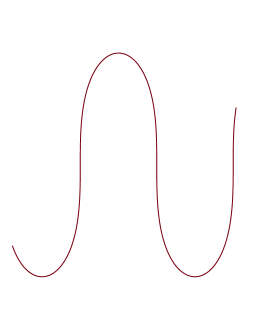
(a) $\sigma_{1}=1,\sigma_{2}=-1,j=1$

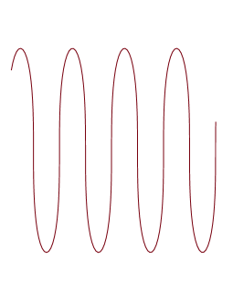
(b) $\sigma_{1}=-1,\sigma_{2}=-1,j=3$

Figure 1. Willmore curves of type $(\sigma_{1},\sigma_{2},j)$

In order to describe the entire solution set $\mathcal{F}$ of the symmetric Navier problem (3) we introduce the solution classes $\mathcal{F}_{0},\mathcal{F}_{1},\ldots$ by setting $\mathcal{F}_{k}:=\mathcal{F}_{k}^{+}\cup\mathcal{F}_{k}^{-}$ and

(5) $$\begin{aligned} \mathcal{F}_{0}^{\pm}&:=\Big{\{}(\gamma,\kappa)\in C^{\infty}([0,1],\mathbb{R}^{2})\times\mathbb{R}:\;\kappa=0,\;\gamma\text{ is the straight line through }A,B\\ &\qquad\qquad\text{or }0\leq\pm\kappa<\infty,\;\gamma\text{ is a }(\mp 1,\pm 1,0)-\text{type solution of \eqref{Gl Navier BVP symm}}\Big{\}},\\ \mathcal{F}_{k}^{\pm}&:=\Big{\{}(\gamma,\kappa)\in C^{\infty}([0,1],\mathbb{R}^{2})\times\mathbb{R}:\;0\leq\pm\kappa<\infty\text{ and }\gamma\text{ is a solution of \eqref{Gl Navier BVP symm}}\\ &\qquad\qquad\text{of type }(\pm 1,\mp 1,k-1)\text{ or }(\mp 1,\pm 1,k)\text{ or }(1,1,k)\text{ or }(-1,-1,k)\Big{\}}.\end{aligned}$$

In our main result Theorem 1 we show amongst other things that every solution of the symmetric Navier problem (3) belongs to precisely one of these sets, in other words we show $\mathcal{F}=\bigcup_{k\in\mathbb{N}_{0}}\mathcal{F}_{k}$ where the union of the right hand side is disjoint. In this decomposition the sets $\mathcal{F}_{1},\mathcal{F}_{2},\ldots$ will turn out to be of similar ”shape” whereas $\mathcal{F}_{0}$ looks different, see figure 2.

Figure 2. An illustration of $\mathcal{F}_{0}$ and $\mathcal{F}_{1}$

Due to space limitations we only illustrated the union of $\mathcal{F}_{0}=\mathcal{F}_{0}^{+}\cup\mathcal{F}_{0}^{-}$ and $\mathcal{F}_{1}=\mathcal{F}_{1}^{+}\cup\mathcal{F}_{1}^{-}$ but the dashed branches emanating from $A_{6},A_{7}$ are intended to indicate that $\mathcal{F}_{1}$ connects to the set $\mathcal{F}_{2}$ which has the same shape as $\mathcal{F}_{1}$ for $(2C,M_{1})$ replaced by $(4C,M_{2})$ and which in turn connects to $\mathcal{F}_{3}$ and so on. Here the real numbers $0<M_{0}<2C<M_{1}<4C<M_{2}<\ldots$ are given by

$$C:=\int_{0}^{1}\frac{4t^{2}}{\sqrt{1-t^{4}}}\,dt,\qquad M_{k}:=\max_{z\in[0,1]}2z\Big{(}kC+2\int_{z}^{1}\frac{t^{2}}{\sqrt{1-t^{4}}}\,dt\Big{)}.$$

The labels $(1,-1,0),(-1,1,0)$, etc. in figure 2 indicate the type of the solution branch which is preserved until one of the bifurcation points $B_{1},B_{2}$ or the trivial solution $A_{1}$ is reached. Let us remark that the horizontal line does not represent a parameter but only enables us to show seven different solutions $A_{1},\ldots,A_{7}$ of (3) for $\kappa=0$ as well as their interconnections in $C^{\infty}([0,1],\mathbb{R}^{2})\times\mathbb{R}$. The solutions $A_{1},A_{2},A_{3}$ belong to $\mathcal{F}_{0}$ whereas $A_{4},A_{5},A_{6},A_{7}$ belong to $\mathcal{F}_{1}$. The above picture indicates that the solution set $\mathcal{F}$ is pathconnected in any reasonable topology. Intending not to overload this paper we do not give a formal proof of this statement but only mention that a piecewise parametrization of the solution sets can be realized using the parameter $z\in[0,1]$ from the proof of Theorem 1. Our result leading to figure 2 reads as follows.

Theorem 1.

Let $A,B\in\mathbb{R}^{2},A\neq B$ and $\kappa\in\mathbb{R}$. Then the following statements concerning the symmetric Navier problem (3) hold true:

• There are

  • precisely three $\mathcal{F}_{0}$-solutions of in case $\kappa=0$,

  • precisely two $\mathcal{F}_{0}$-solutions of in case $0<|\kappa|\|B-A\|<M_{0}$,

  • precisely one $\mathcal{F}_{0}$-solution in case $|\kappa|\|B-A\|=M_{0}$,

  • no $\mathcal{F}_{0}$-solutions in case $|\kappa|\|B-A\|>M_{0}$

• and for all $k\geq 1$ there are

  • precisely four $\mathcal{F}_{k}$-solutions in case $|\kappa|\|B-A\|<2kC$,

  • precisely two $\mathcal{F}_{k}$-solutions in case $2kC\leq|\kappa|\|B-A\|<M_{k}$,

  • precisely one $\mathcal{F}_{k}$-solution in case $|\kappa|\|B-A\|=M_{k}$,

  • no $\mathcal{F}_{k}$-solutions in case $|\kappa|\|B-A\|>M_{k}$.

• The minimal energy solutions of (3) are given as follows:

  • In case $\kappa=0$ the Willmore minimizer is the straight line joining $A$ and $B$.

  • In case $2kC<|\kappa|\|B-A\|\leq M_{k}$ for some $k\in\mathbb{N}_{0}$ the Willmore minimizer is of type $(-\operatorname{sign}(\kappa),\operatorname{sign}(\kappa),k)$.

  • In case $M_{k}<|\kappa|\|B-A\|\leq 2(k+1)C$ for some $k\in\mathbb{N}_{0}$ the Willmore minimizer is the unique solution of type $(\operatorname{sign}(\kappa),-\operatorname{sign}(\kappa),k)$.

• All $(\sigma_{1},\sigma_{2},j)$-type solutions with $\sigma_{1}=-\sigma_{2}$ are axially symmetric. The $(\sigma_{1},\sigma_{2},j)$-type solutions with $\sigma_{1}=\sigma_{2}$ are not axially symmetric and pointwise symmetric only in case $\kappa=0$.

We would like to point out that we can write down almost explicit formulas for the solutions obtained in Theorem 1 using the formulas from our general result which we will provide in Theorem 3 and the subsequent Remark 2 (b). Futhermore let us notice that the proof of Theorem 1 (ii) (b) reveals which of the two $(-\operatorname{sign}(\kappa),\operatorname{sign}(\kappa),k)$-type solutions is the Willmore minimizer. We did not provide this piece of information in the above statement in order not to anticipate the required notation. At this stage let us only remark that in figure 2 the Willmore minimizers from Theorem 1 (ii) (b) lie on the left parts of the branches consisting of $(-\operatorname{sign}(\kappa),\operatorname{sign}(\kappa),0)$-type respectively $(-\operatorname{sign}(\kappa),\operatorname{sign}(\kappa),1)$-type solutions.

Remark 1.

• The numerical value for $M_{0}$ is $1.34380$ which is precisely the threshold value found in Theorem 1 in [2]. The existence result for graph-type solutions from [2] are therefore reproduced by Theorem 1 (i)(b)-(d). Notice that a $(\sigma_{1},\sigma_{2},j)$-type solution with $j\geq 1$ can not be a graph with respect to any coordinate frame. On the other hand, in (i)(a) we found three $\mathcal{F}_{0}$-solutions for $\kappa=0$ which are the straight line and two nontrivial Willmore curves of type $(1,-1,0)$ respectively $(-1,1,0)$. The latter two solutions were not discovered by Deckelnick and Grunau because they are continuous but non-smooth graphs since the slopes (calculated with respect to the straight line joining the end points of the curve) at both end points are $+\infty$ or $-\infty$. Viewed as a curve, however, these solutions are smooth.

• From Theorem 1 (i) one deduces that for all $\kappa$ and all $A\neq B$ there is an infinite sequence of Willmore curves solving (3) whose Willmore energies tends to $+\infty$. Here one uses that the Willmore energies of $\mathcal{F}_{k}-$solutions tend to $+\infty$ as $k\to\infty$. We will see in Theorem 2 that this result remains true in the nonsymmetric case.

• Using the formula for the length of a Willmore curve from our general result Theorem 3 one can show that for any given $A,B\in\mathbb{R}^{2},\kappa\in\mathbb{R}$ satisfying $A\neq B,\kappa\neq 0$ the solution of (3) having minimal length $L$ must be of type $(-\operatorname{sign}(\kappa),\operatorname{sign}(\kappa),j)$ for some $j\in\mathbb{N}_{0}$. More precisely, defining $L^{*}:=T\|B-A\|/(\sqrt{2}C)$ for the periodicity $T$ of $\operatorname{cn}$ (see section 2) one can show $L>L^{*},L=L^{*},L<L^{*}$ respectively if the solution curve is of type $(\sigma_{1},\sigma_{2},j)$ with $\sigma_{1}=-\sigma_{2}=\operatorname{sign}(\kappa),\sigma_{1}=\sigma_{2},\sigma_{1}=-\sigma_{2}=-\operatorname{sign}(\kappa)$. Notice that in the case $\|B-A\|=1$ studied by Linnér we have $L^{*}\approx 2.18844$ which is precisely the value on page 460 in Linnér’s paper [5]. Numerical plots indicate that in most cases the Willmore curves of minimal length have to be of type $(-\operatorname{sign}(\kappa),\operatorname{sign}(\kappa),j)$ where $j$ is smallest possible which, however, is not true in general as the following numerical example shows. In the special case $\|B-A\|=1,\kappa=9.885$ there is a $(-1,1,2)$-type solution generated by $a\approx 7.48526$ having length $L_{1}\approx 2.08043$ and a $(-1,1,3)$-type solution generated by $a\approx 11.65140$ which has length $L_{2}\approx 2.08018$ and we observe $L_{2}<L_{1}$.

• Having a look at figure 2 we find that the set of Willmore minimizers described in Theorem 1 (ii) is not connected as a whole, but it is path-connected within suitable intervals of the parameter $\kappa\|B-A\|$.

In the nonsymmetric case $\kappa_{1}\neq\kappa_{2}$ it seems to be difficult to identify nicely behaved connected sets which constitute the whole solution set. However, we find existence and multiplicity results in the spirit of Remark 1 (b). We can prove the following result.

Theorem 2.

Let $A,B\in\mathbb{R}^{2},\kappa_{1},\kappa_{2}\in\mathbb{R}$ satisfy $A\neq B,\kappa_{1}\neq\kappa_{2}$ and let $\sigma_{1},\sigma_{2}\in\{-1,+1\}$. Then there is a smallest natural number $j_{0}$ such that for all $j\geq j_{0}$ the Navier problem (2) has at least one $(\sigma_{1},\sigma_{2},j)$-type solution $\gamma_{j}$ such that $W(\gamma_{j_{0}})<W(\gamma_{j_{0}+1})<\ldots<W(\gamma_{j})\to+\infty$ as $j\to\infty$. Moreover, we have $j_{0}\leq j_{0}^{*}$ where $j_{0}^{*}$ is the smallest natural number satisfying

$$\|B-A\|^{2}\leq\begin{cases}\frac{4C^{2}(j_{0}^{*}-\frac{1}{2})^{2}}{\max\{\kappa_{1}^{2},\kappa_{2}^{2}\}}+\frac{4(\kappa_{2}-\kappa_{1})^{2}}{\max\{\kappa_{1}^{4},\kappa_{2}^{4}\}}&,\text{if }\sigma_{1}=\sigma_{2}\\ \frac{4C^{2}(j_{0}^{*}-1)^{2}}{\max\{\kappa_{1}^{2},\kappa_{2}^{2}\}}+\frac{4(\kappa_{2}-\kappa_{1})^{2}}{\max\{\kappa_{1}^{4},\kappa_{2}^{4}\}}&,\text{if }\sigma_{1}=-\sigma_{2}.\end{cases}$$

The proof of both theorems will be achieved by using an explicit expression for Willmore curves like the ones used in Linnér’s work [5] and Singer’s lectures [7]. In Proposition 1 we show that the set of Willmore curves emanating from $A\in\mathbb{R}^{2}$ is generated by four real parameters so that solving the Navier problem is reduced to adjusting these parameters in such a way that the four equations given by the boundary conditions are satisfied. The proofs of Theorem 1 and Theorem 2 will therefore be based on explicit computations which even allow to write down the complete solution theory for the general Navier problem (2), see Theorem 3. Basically the same strategy can be pursued to solve the general Dirichlet problem (1). In view of the fact that a discussion of this boundary value problem does not reveal any new methodological aspect we decided to defer it to Appendix B. Notice that even in the presumably simplest special cases $\theta_{2}-\theta_{1}\in\{-\pi/2,0,\pi/2\}$ it requires non-negligible computational effort to prove optimal existence and multiplicity results for (1) like the ones in Theorem 1. We want to stress that it would be desirable to prove the existence of infinitely many solutions of the Navier problem and the Dirichlet problem also in higher dimensions where Willmore curves $\gamma\in C^{\infty}([0,1],\mathbb{R}^{n})$ with $n\geq 3$ are considered. It would be very interesting to compare such a solution theory to the corresponding theory for Willmore surfaces established by Schätzle [6] where the existence of one solution of the corresponding Dirichlet problem is proved.

Let us finally outline how this paper is organized. In section 2 we review some preliminary facts about Willmore curves and Jacobi’s elliptic functions appearing in the definition of $\kappa_{a,b}$, see (4). Next, in section 3, we provide all information concerning the Navier problem starting with a derivation of the complete solution theory for the general Navier problem (2) in subsection 3.1. In the subsections 3.2 and 3.3 this result will be applied to the special cases $\kappa_{1}=\kappa_{2}$ respectively $\kappa_{1}\neq\kappa_{2}$ in order to prove Theorem 1 and Theorem 2. In Appendix A we provide the proof of one auxiliary result (Proposition 1) and Appendix B is devoted to the solution theory for the general Dirichlet problem.

2. Preliminaries

The Willmore functional is invariant under reparametrization so that the arc-length parametrization $\hat{\gamma}$ of a given Willmore curve $\gamma$ is also a Willmore curve. It is known that the curvature function $\hat{\kappa}$ of $\hat{\gamma}$ satisfies the ordinary differential equation

(6) $$-\hat{\kappa}^{\prime\prime}(s)=\frac{1}{2}\hat{\kappa}(s)^{3},$$

in particular it is not restrictive to consider smooth curves only. A derivation of (6) may be found in Singer’s lectures [7]. Moreover, we will use the fact that every regular planar curve $\gamma\in C^{\infty}([0,1],\mathbb{R}^{2})$ admits the representation

(7) $$\begin{aligned} \gamma\sim\hat{\gamma},\qquad\hat{\gamma}(t)=A+Q\int_{0}^{t}\begin{pmatrix}\cos(\int_{0}^{s}\hat{\kappa}(r)\,dr)\\ \sin(\int_{0}^{s}\hat{\kappa}(r)\,dr)\\ \end{pmatrix}\,ds\qquad(t\in[0,L])\end{aligned}$$

where $A$ is a point in $\mathbb{R}^{2}$ and $Q\in SO(2)$ is a rotation matrix. Here we used the symbol $\gamma\sim\hat{\gamma}$ in order to indicate that $\gamma,\hat{\gamma}$ can be transformed into each other by some diffeomorphic reparametrization. In Proposition 1 we will show that a regular curve $\gamma$ is a Willmore curve if and only if the function $\hat{\kappa}$ in (7) is given by $\hat{\kappa}=\kappa_{a,b}$ for $\kappa_{a,b}$ as in (4) with ${a\geq 0},{L>0},{-T/2\leq b<T/2}$. In such a situation we will say that the parameters $a,b,L$ are admissible. Since this fact is fundamental for the proofs of our results we mention some basic properties of Jacobi’s elliptic functions $\operatorname{sn},\operatorname{cn},\operatorname{dn}$. Each of these functions maps $\mathbb{R}$ into the interval $[-1,1]$ and is $T$-periodic where $T:=4\int_{0}^{1}(\tfrac{2}{1-t^{4}})^{1/2}\,dt\approx 7.41630$. We will use the identities $\operatorname{cn}^{4}+2\operatorname{sn}^{2}\operatorname{dn}^{2}=1$ and $\operatorname{cn}^{\prime}=-\operatorname{sn}\operatorname{dn}$ on $\mathbb{R}$ as well as $\arccos(\operatorname{cn}^{2})^{\prime}=\sqrt{2}\operatorname{cn}$ on $[0,T/2]$. Moreover we will exploit the fact that $\operatorname{cn}$ is $T/2$-antiperiodic, i.e. $\operatorname{cn}(x+T/2)=-\operatorname{cn}(x)$ for all $x\in\mathbb{R}$, and that $\operatorname{cn}$ is decreasing on $[0,T/2]$ with inverse function $\operatorname{cn}^{-1}$ satisfying $\operatorname{cn}^{-1}(1)=0$ and $(\operatorname{cn}^{-1})^{\prime}(t)=-(\tfrac{2}{1-t^{4}})^{1/2}$ for $t\in(-1,1)$.

3. The Navier problem

3.1. The general result

The Navier boundary value problem (2) does not appear to be easily solvable since the curvature function $\det(\gamma^{\prime},\gamma^{\prime\prime})|\gamma^{\prime}|^{-3}$ of a given regular smooth curve $\gamma$ does in general not solve a reasonable differential equation. If, however, we parametrize $\gamma$ by arc-length we obtain a smooth regular curve $\hat{\gamma}:[0,L]\to\mathbb{R}^{2}$ whose curvature function $\hat{\kappa}$ satisfies the differential equation $-2\hat{\kappa}^{\prime\prime}=\hat{\kappa}^{3}$ on $[0,L]$ which is explicitly solvable. Indeed, in Proposition 1 we will show that the nontrivial solutions of this differential equation are given by the functions $\kappa_{a,b}$ from (4) so that the general form of a Willmore curve $\gamma$ is given by

(8) $$\begin{aligned} \gamma\sim\hat{\gamma},\qquad\hat{\gamma}(t)&=A+Q\int_{0}^{t}\begin{pmatrix}\cos(\int_{0}^{s}\kappa_{a,b}(r)\,dr)\\ \sin(\int_{0}^{s}\kappa_{a,b}(r)\,dr)\\ \end{pmatrix}\,ds\qquad\text{for all }t\in[0,L]\end{aligned}$$

where $Q\in SO(2)$ is a rotation matrix and $L>0$ denotes the length of $\gamma$. In such a situation we will say that the Willmore curve $\gamma$ is generated by $a,b,L$. As a consequence, a Willmore curve $\gamma$ solves the Navier boundary value problem (2) once we determine the parameters $a,b,L,Q$ such that the equations

(9) $$\hat{\gamma}(L)-\hat{\gamma}(0)=B-A,\qquad\kappa_{a,b}(0)=\kappa_{1},\qquad\kappa_{a,b}(L)=\kappa_{2},$$

are satisfied. Summarizing the above statements and taking into account Definition 2 we obtain the following preliminary result the proof of which we defer to Appendix A.

Proposition 1.

Let $\gamma\in C^{\infty}([0,1],\mathbb{R}^{2})$ be a regular curve. Then the following is true:

• The curve $\gamma$ solves the Navier problem (2) if and only if $\gamma$ is given by (8) for admissible parameters $a,b,L$ and $Q\in SO(2)$ satisfying (9).

• Let $\sigma_{1},\sigma_{2}\in\{-1,+1\},j\in\mathbb{N}_{0}$ be given and assume $\gamma$ satisfies (8). Then $\gamma$ is of type $(\sigma_{1},\sigma_{2},j)$ if and only if there is some $\tilde{b}\in[-T/2,T/2)$ such that

  (10) $$\begin{aligned} b+aL=(j+\lceil(b-\tilde{b})/T\rceil)T+\tilde{b},\qquad\operatorname{sign}(b)=\sigma_{1},\qquad\operatorname{sign}(\tilde{b})=\sigma_{2}.\end{aligned}$$

In Theorem 3 we provide the complete solution theory for the boundary value problem (2) which, due to Proposition 1, is reduced to solving the equivalent problem (9). In order to write down the precise conditions when $(\sigma_{1},\sigma_{2},j)$-type solutions of (2) exist we need the functions

(11) $$\begin{aligned} f_{\sigma_{1},\sigma_{2},j}(\kappa_{1},\kappa_{2},a)&:=\Big{(}j+\Big{\lceil}\frac{\sigma_{1}\operatorname{cn}^{-1}(\frac{\kappa_{1}}{\sqrt{2}a})-\sigma_{2}\operatorname{cn}^{-1}(\frac{\kappa_{2}}{\sqrt{2}a})}{T}\Big{\rceil}\Big{)}\cdot C\\ &-\sigma_{1}\begin{cases}\int_{\frac{\kappa_{1}}{\sqrt{2}a}}^{\frac{\kappa_{2}}{\sqrt{2}a}}\frac{t^{2}}{\sqrt{1-t^{4}}}\,dt&,\text{if }\sigma_{1}=\sigma_{2}\\ \int_{\frac{\kappa_{1}}{\sqrt{2}a}}^{1}\frac{t^{2}}{\sqrt{1-t^{4}}}\,dt+\int_{\frac{\kappa_{2}}{\sqrt{2}a}}^{1}\frac{t^{2}}{\sqrt{1-t^{4}}}\,dt&,\text{if }\sigma_{1}\neq\sigma_{2}\end{cases}\end{aligned}$$

where $\kappa_{1},\kappa_{2}\in\mathbb{R}$ and $a\geq a_{0}:=\max\{|\kappa_{1}|,|\kappa_{2}|\}/\sqrt{2}$.

Theorem 3.

Let $A,B\in\mathbb{R}^{2},A\neq B$ and $\kappa_{1},\kappa_{2}\in\mathbb{R}$ be given, let $\sigma_{1},\sigma_{2}\in\{-1,+1\},{j\in\mathbb{N}_{0}}$. Then all solutions of the Navier problem (2) which are regular curves of type $(\sigma_{1},\sigma_{2},j)$ are given by (8) for $a,b,L$ and the uniquely determined rotation matrix $Q\in SO(2)$ satisfying

(12) $$\begin{aligned} b&=\sigma_{1}\operatorname{cn}^{-1}\Big{(}\frac{\kappa_{1}}{\sqrt{2}a}\Big{)},\qquad\qquad Q^{T}(B-A)=\int_{0}^{L}\begin{pmatrix}\cos(\int_{0}^{s}\kappa_{a,b}(r))\,dr\\ \sin(\int_{0}^{s}\kappa_{a,b}(r))\,dr\\ \end{pmatrix},\\ L&=\frac{1}{a}\Big{(}\Big{(}j+\Big{\lceil}\frac{\sigma_{1}\operatorname{cn}^{-1}(\frac{\kappa_{1}}{\sqrt{2}a})-\sigma_{2}\operatorname{cn}^{-1}(\frac{\kappa_{2}}{\sqrt{2}a})}{T}\Big{\rceil}\Big{)}T+\sigma_{2}\operatorname{cn}^{-1}\Big{(}\frac{\kappa_{2}}{\sqrt{2}a}\Big{)}-\sigma_{1}\operatorname{cn}^{-1}\Big{(}\frac{\kappa_{1}}{\sqrt{2}a}\Big{)}\Big{)}\end{aligned}$$

where $a$ is any solution of

(13) $$\begin{aligned} \|B-A\|^{2}=\frac{2}{a^{2}}f_{\sigma_{1},\sigma_{2},j}(\kappa_{1},\kappa_{2},a)^{2}+\frac{(\kappa_{2}-\kappa_{1})^{2}}{a^{4}}\qquad(a>0,a\geq a_{0})\\ \text{provided}\quad\kappa_{1}=\pm\sqrt{2}a\Rightarrow\sigma_{1}=\pm 1,\quad\kappa_{2}=\pm\sqrt{2}a\Rightarrow\sigma_{2}=\pm 1.\end{aligned}$$

The Willmore energy of such a curve $\gamma$ is given by

$$W(\gamma)=\big{(}a^{4}\|B-A\|^{2}-(\kappa_{2}-\kappa_{1})^{2}\big{)}^{1/2}$$

Proof.

By Proposition 1 we have to find all admissible parameters $a,b,L$ satisfying (10) and a rotation matrix $Q\in SO(2)$ such that the equation (9) holds. We show that all these parameters are given by (12) and (13) and it is a straightforward calculation (which we omit) to check that parameters given by these equations indeed give rise to a $(\sigma_{1},\sigma_{2},j)$-type solution of (9). So let us in the following assume that $a,b,L,Q$ solve (9). Notice that we have $a>0$ by assumption, i.e. $\gamma$ is not the straight line.

First let us remark that the boundary conditions $\kappa_{a,b}(0)=\kappa_{1},\kappa_{a,b}(L)=\kappa_{2}$ imply

(14) $$\operatorname{cn}(b)=\frac{\kappa_{1}}{\sqrt{2}a},\qquad\operatorname{cn}(b+aL)=\frac{\kappa_{2}}{\sqrt{2}a}.$$

so that $|\operatorname{cn}|\leq 1$ gives $\sqrt{2}a\geq\max\{|\kappa_{1}|,|\kappa_{2}|\}$ and thus $a\geq a_{0}$.

1st step: Simplification.  From (9) we infer

$$\|B-A\|^{2} =\|\hat{\gamma}(L)-\hat{\gamma}(0)\|^{2}$$

$$=\Big{\|}\int_{0}^{L}Q\begin{pmatrix}\cos(\int_{0}^{s}\kappa_{a,b}(r)\,dr)\\ \sin(\int_{0}^{s}\kappa_{a,b}(r)\,dr)\\ \end{pmatrix}\,ds\Big{\|}^{2}$$

$$=\Big{\|}\int_{0}^{L}\begin{pmatrix}\cos(\int_{0}^{s}\kappa_{a,b}(r)\,dr)\\ \sin(\int_{0}^{s}\kappa_{a,b}(r)\,dr)\\ \end{pmatrix}\,ds\Big{\|}^{2}$$

(15) $$=\Big{(}\int_{0}^{L}\cos\Big{(}\int_{0}^{s}\kappa_{a,b}(r)\,dr\Big{)}\,ds\Big{)}^{2}+\Big{(}\int_{0}^{L}\sin\Big{(}\int_{0}^{s}\kappa_{a,b}(r)\,dr\Big{)}\,ds\Big{)}^{2}$$

Using the identities

$$\frac{d}{dr}\Big{(}2\arctan\Big{(}\frac{\operatorname{sn}(ar+b)}{\sqrt{2}\operatorname{dn}(ar+b)}\Big{)}\Big{)} =\sqrt{2}a\operatorname{cn}(ar+b)=\kappa_{a,b}(r)\qquad(r\in\mathbb{R}),$$

$$\cos(2\arctan(x)-2\arctan(y)) =\frac{2(1+xy)^{2}}{(1+x^{2})(1+y^{2})}-1\;\;\qquad(x,y\in\mathbb{R}),$$

$$\sin(2\arctan(x)-2\arctan(y)) =\frac{2(1+xy)(x-y)}{(1+x^{2})(1+y^{2})}\qquad\qquad(x,y\in\mathbb{R})$$

we obtain after some rearrangements

(16) $$\begin{aligned} \cos\Big{(}\int_{0}^{s}\kappa_{a,b}(r)\,dr\Big{)}&=\operatorname{cn}(b)^{2}\operatorname{cn}(as+b)^{2}+2\operatorname{sn}(b)\operatorname{dn}(b)\operatorname{sn}(as+b)\operatorname{dn}(as+b),\\ \sin\Big{(}\int_{0}^{s}\kappa_{a,b}(r)\,dr\Big{)}&=-\sqrt{2}\operatorname{sn}(b)\operatorname{dn}(b)\operatorname{cn}(as+b)^{2}+\sqrt{2}\operatorname{cn}(b)^{2}\operatorname{sn}(as+b)\operatorname{dn}(as+b).\end{aligned}$$

In order to proceed with calculating $\|B-A\|^{2}$ we set

(17) $$\alpha:=\int_{0}^{L}\operatorname{cn}(as+b)^{2}\,ds,\qquad\beta:=\int_{0}^{L}\sqrt{2}\operatorname{sn}(as+b)\operatorname{dn}(as+b)\,ds.$$

so that (3.1),(16) yield

(18) $$\begin{aligned} \|B-A\|^{2}&=\Big{(}\operatorname{cn}(b)^{2}\alpha+\sqrt{2}\operatorname{sn}(b)\operatorname{dn}(b)\beta\Big{)}^{2}+\Big{(}-\sqrt{2}\operatorname{sn}(b)\operatorname{dn}(b)\alpha+\operatorname{cn}(b)^{2}\beta\Big{)}^{2}\\ &=\alpha^{2}(\operatorname{cn}(b)^{4}+2\operatorname{sn}(b)^{2}\operatorname{cn}(b)^{2})+\beta^{2}(\operatorname{cn}(b)^{4}+2\operatorname{sn}(b)^{2}\operatorname{dn}(b)^{2})\\ &=\alpha^{2}+\beta^{2}\\ &\stackrel{{\scriptstyle\eqref{Gl metaThm 3}}}{{=}}\frac{1}{a^{2}}\Big{(}\int_{b}^{b+aL}\operatorname{cn}(t)^{2}\,dt\Big{)}^{2}+\Big{(}\Big{[}-\frac{\sqrt{2}}{a}\operatorname{cn}(as+b)\Big{]}^{L}_{0}\Big{)}^{2}\\ &\stackrel{{\scriptstyle\eqref{Gl metaThm 0}}}{{=}}\frac{1}{a^{2}}\Big{(}\int_{b}^{b+aL}\operatorname{cn}(t)^{2}\,dt\Big{)}^{2}+\frac{(\kappa_{2}-\kappa_{1})^{2}}{a^{4}}.\end{aligned}$$

In order to derive equation (13) it therefore remains to show

(19) $$\frac{1}{\sqrt{2}}\int_{b}^{b+aL}\operatorname{cn}(t)^{2}\,dt=f_{\sigma_{1},\sigma_{2},j}(\kappa_{1},\kappa_{2},a).$$

2nd step: Proving (19).  For notational convenience we define $\tilde{\kappa}_{1}:=\kappa_{1}/(\sqrt{2}a),{\tilde{\kappa}_{2}:=\kappa_{2}/(\sqrt{2}a)}$ so that $a\geq a_{0}$ implies $\tilde{\kappa}_{1},\tilde{\kappa}_{2}\in[-1,1]$. Then (10) and the boundary conditions (14) yield

(20) $$\begin{aligned} b&=\sigma_{1}\operatorname{cn}^{-1}(\tilde{\kappa}_{1}),\qquad\quad\tilde{\kappa}_{1}=\pm 1\Rightarrow\sigma_{1}=\pm 1\\ \tilde{b}&=\sigma_{2}\operatorname{cn}^{-1}(\tilde{\kappa}_{2}),\qquad\quad\tilde{\kappa}_{2}=\pm 1\Rightarrow\sigma_{2}=\pm 1.\end{aligned}$$

Using the shorthand notation $m:=j+\lceil(b-\tilde{b})/T\rceil$ we obtain

$$\;\frac{1}{\sqrt{2}}\int_{b}^{b+aL}\operatorname{cn}(t)^{2}\,dt$$

$$=\frac{1}{\sqrt{2}}\int_{\sigma_{1}\operatorname{cn}^{-1}(\tilde{\kappa}_{1})}^{mT+\sigma_{2}\operatorname{cn}^{-1}(\tilde{\kappa}_{2})}\operatorname{cn}(t)^{2}\,dt$$

$$=\frac{m}{\sqrt{2}}\int_{0}^{T}\operatorname{cn}(t)^{2}\,dt+\frac{1}{\sqrt{2}}\int_{\sigma_{1}\operatorname{cn}^{-1}(\tilde{\kappa}_{1})}^{\sigma_{2}\operatorname{cn}^{-1}(\tilde{\kappa}_{2})}\operatorname{cn}(t)^{2}\,dt$$

$$=2\sqrt{2}m\int_{0}^{T/4}\operatorname{cn}(t)^{2}\,dt+\frac{\sigma_{1}}{\sqrt{2}}\begin{cases}\int_{\operatorname{cn}^{-1}(\tilde{\kappa}_{1})}^{\operatorname{cn}^{-1}(\tilde{\kappa}_{2})}\operatorname{cn}(t)^{2}\,dt&,\text{if }\sigma_{1}=\sigma_{2}\\ -\int_{0}^{\operatorname{cn}^{-1}(\tilde{\kappa}_{1})}\operatorname{cn}(t)^{2}\,dt-\int_{0}^{\operatorname{cn}^{-1}(\tilde{\kappa}_{2})}\operatorname{cn}(t)^{2}\,dt&,\text{if }\sigma_{1}\neq\sigma_{2}\end{cases}$$

$$=2\sqrt{2}m\int_{0}^{1}t^{2}\sqrt{\frac{2}{1-t^{4}}}\,dt-\frac{\sigma_{1}}{\sqrt{2}}\begin{cases}\int_{\tilde{\kappa}_{1}}^{\tilde{\kappa}_{2}}t^{2}\sqrt{\frac{2}{1-t^{4}}}\,dt&,\text{if }\sigma_{1}=\sigma_{2}\\ \int_{\tilde{\kappa}_{1}}^{1}t^{2}\sqrt{\frac{2}{1-t^{4}}}\,dt+\int_{\tilde{\kappa}_{2}}^{1}t^{2}\sqrt{\frac{2}{1-t^{4}}}\,dt&,\text{if }\sigma_{1}\neq\sigma_{2}\end{cases}$$

$$=mC-\sigma_{1}\begin{cases}\int_{\tilde{\kappa}_{1}}^{\tilde{\kappa}_{2}}\frac{t^{2}}{\sqrt{1-t^{4}}}\,dt&,\text{if }\sigma_{1}=\sigma_{2},\\ \int_{\tilde{\kappa}_{1}}^{1}\frac{t^{2}}{\sqrt{1-t^{4}}}\,dt+\int_{\tilde{\kappa}_{2}}^{1}\frac{t^{2}}{\sqrt{1-t^{4}}}\,dt&,\text{if }\sigma_{1}\neq\sigma_{2}\end{cases}$$

$$=f_{\sigma_{1},\sigma_{2},j}(\kappa_{1},\kappa_{2},a).$$

The formulas for $L$ and $W$ follow from (10) and (20):

(21) $$\begin{aligned} L&=\frac{1}{a}\big{(}(j+\lceil(b-\tilde{b})/T\rceil)T+\tilde{b}-b\big{)}\\ &=\frac{1}{a}\Big{(}\Big{(}j+\Big{\lceil}\frac{\sigma_{1}\operatorname{cn}^{-1}(\tilde{\kappa}_{1})-\sigma_{2}\operatorname{cn}^{-1}(\tilde{\kappa}_{2})}{T}\Big{\rceil}\Big{)}T+\sigma_{2}\operatorname{cn}^{-1}(\tilde{\kappa}_{2})-\sigma_{1}\operatorname{cn}^{-1}(\tilde{\kappa}_{1})\Big{)},\\ W&=\frac{1}{2}\int_{\gamma}\kappa_{\gamma}^{2}\;=\;\frac{1}{2}\int_{0}^{L}\kappa_{a,b}(s)^{2}\,ds\;=\;a^{2}\int_{0}^{L}\operatorname{cn}(as+b)^{2}\,ds\\ &\stackrel{{\scriptstyle\eqref{Gl metaThm 3}}}{{=}}a^{2}\cdot\alpha\;\stackrel{{\scriptstyle\eqref{Gl metaThm 6}}}{{=}}\;a^{2}\cdot(\|B-A\|^{2}-\beta^{2})^{1/2}\\ &=\big{(}a^{4}\|B-A\|^{2}-(\kappa_{2}-\kappa_{1})^{2}\big{)}^{1/2}.\end{aligned}$$

$\Box$

Remark 2.

• Reviewing the proof of Theorem 3 one finds that the boundary value problem (2) does not have nontrivial solutions in case $A=B$, i.e. there are no closed Willmore curves. This result has already been obtained by Linnér, cf. Proposition 3 in [5]. In fact, (18) would imply $aL=0$ so that the solution must be the ”trivial curve” consisting of precisely one point.

• For computational purposes it might be interesting to know that the integrals involved in the definition of $Q$ need not be calculated numerically. With some computational effort one finds that $Q$ is the unique rotation matrix satisfying $Qw=B-A$ where the vector $w=(w_{1},w_{2})\in\mathbb{R}^{2}$ is given by

  $$w_{1} =\frac{\kappa_{1}^{2}(a^{4}\|B-A\|^{2}-(\kappa_{2}-\kappa_{1})^{4})^{1/2}+\sigma_{1}(\kappa_{1}-\kappa_{2})(4a^{4}-\kappa_{1}^{4})^{1/2}}{2a^{4}},$$

  $$w_{2} =\frac{-\sigma_{1}((4a^{4}-\kappa_{1}^{4})(a^{4}\|B-A\|^{2}-(\kappa_{2}-\kappa_{1})^{4}))^{1/2}+\kappa_{1}^{2}(\kappa_{1}-\kappa_{2})}{2a^{4}}.$$

  Hence, $Q$ can be expressed in terms of $B-A,w_{1},w_{2}$ only.

3.2. Proof of Theorem 1

3.2.1. Proof of Theorem 1 (i) - Existence results

In order to prove Theorem 1 (i) we apply Theorem 3 to the special case $\kappa_{1}=\kappa_{2}=\kappa$. As before we set $\sqrt{2}a_{0}:=\max\{|\kappa_{1}|,|\kappa_{2}|\}=|\kappa|$. Theorem 3 tells us that $a>0,a\geq a_{0}$ generates a solution of type $(\sigma_{1},\sigma_{2},j)$ if and only if

$$\begin{aligned} \|B-A\|&=\frac{\sqrt{2}}{a}f_{\sigma_{1},\sigma_{2},j}(\kappa,\kappa,a)\\ &=\frac{\sqrt{2}}{a}\Big{(}\Big{(}j+\Big{\lceil}\frac{(\sigma_{1}-\sigma_{2})\operatorname{cn}^{-1}(\frac{\kappa}{\sqrt{2}a})}{T}\Big{\rceil}\Big{)}C-\sigma_{1}\begin{cases}0&,\text{if }\sigma_{1}=\sigma_{2},\\ 2\int_{\frac{\kappa}{\sqrt{2}a}}^{1}\frac{t^{2}}{\sqrt{1-t^{4}}}\,dt&,\text{if }\sigma_{1}\neq\sigma_{2}\end{cases}\Big{)}\\ &=\frac{\sqrt{2}}{a}\cdot\begin{cases}jC&,\text{if }\sigma_{1}=\sigma_{2}\text{ or }(\sigma_{1},\sigma_{2},\frac{\kappa}{\sqrt{2}a})=(-1,1,-1),\\ jC+2\int_{\frac{\sigma_{2}\kappa}{\sqrt{2}a}}^{1}\frac{t^{2}}{\sqrt{1-t^{4}}}\,dt&,\text{if }\sigma_{1}\neq\sigma_{2}\text{ and }(\sigma_{1},\sigma_{2},\frac{\kappa}{\sqrt{2}a})\neq(-1,1,-1)\end{cases}\end{aligned}$$

provided $|\kappa|=\sqrt{2}a$ implies $\sigma_{1}=\sigma_{2}=\operatorname{sign}(\kappa)$. Hence, the above equation is equivalent to
 
 

()_j

$$\|B-A\|=\frac{\sqrt{2}}{a}\cdot\begin{cases}jC&,\text{if }\sigma_{1}=\sigma_{2},\\ jC+2\int_{\frac{\sigma_{2}\kappa}{\sqrt{2}a}}^{1}\frac{t^{2}}{\sqrt{1-t^{4}}}\,dt&,\text{if }\sigma_{1}\neq\sigma_{2}\end{cases}$$

$$\text{provided}\quad|\kappa|=\sqrt{2}a\Rightarrow\sigma_{1}=\sigma_{2}=\operatorname{sign}(\kappa)$$

so that it remains to determine all solutions $a>0,a\geq a_{0}$ of (22)_j. First let us note that there are no $(\sigma_{1},\sigma_{2},0)$-type solutions with $\sigma_{1}=\sigma_{2}$, see (22)₀. Hence, by definition of the sets $\mathcal{F}_{0},\mathcal{F}_{1},\ldots,$ all solutions of the symmetric Navier problem (3) are contained in $\bigcup_{k=0}^{\infty}\mathcal{F}_{k}$ which shows $\mathcal{F}=\bigcup_{k=0}^{\infty}\mathcal{F}_{k}$. In order to prove the existence and nonexistence results stated in Theorem 1 it therefore remains to find all solutions belonging to $\mathcal{F}_{k}=\mathcal{F}_{k}^{+}\cup\mathcal{F}_{k}^{-}$ for any given $k\in\mathbb{N}_{0}$. In the following we will without loss of generality restrict ourselves to the case $\kappa\geq 0$. This is justified since every $(\sigma_{1},\sigma_{2},j)$-type solution of (3) generated by $a,b,L$ gives rise to a $(-\sigma_{1},-\sigma_{2},j)$-type solution of (3) with $\kappa$ replaced by $-\kappa$ which is generated by $a,b-\sigma_{1}T/2,L$. Let us recall that figure 2 might help to understand and to visualize the proof of Theorem 1 (i).

Proof of Theorem 1 (i)(a)-(d):  First we determine all solutions belonging to $\mathcal{F}_{0}^{+}$. All solutions from $\mathcal{F}_{0}^{+}$ with $\kappa=0$ are the straight line from $A$ to $B$ and the solution of type $(-1,1,0)$ which is generated by $a=C(\sqrt{2}\|B-A\|)^{-1}$, see (22). The solutions from $\mathcal{F}_{0}^{+}$ with $\kappa>0$ are of type $(-1,1,0)$ and therefore generated by $a>0,a\geq a_{0}$ such that

(23) $$\kappa\|B-A\|=4z\int_{z}^{1}\frac{t^{2}}{\sqrt{1-t^{4}}}\,dt\qquad\text{where }z=\frac{\kappa}{\sqrt{2}a}\in(0,1),$$

see (22). Notice that $z>0$ is due to the assumption $\kappa>0$ whereas $z\leq 1$ follows from $a\geq a_{0}$ and $z\neq 1$ follows from the last line in (22). The function defined by the right hand side is positive and strictly concave on $(0,1)$ with global maximum $M_{0}$. Hence, we find two, one respectively no solution in $\mathcal{F}_{0}^{+}$ according to $\kappa\|B-A\|$ being smaller than, equal to or larger than $M_{0}$. This proves the assertions (i)(a)-(d) in Theorem 1.

Proof of Theorem 1 (i)(e)-(h):  Now we investigate the solutions belonging to $\mathcal{F}_{k}^{+}$ for $k\geq 1$. From (22) we infer that solutions of type $(\sigma_{1},\sigma_{2},k)$ with $\sigma_{1}=\sigma_{2}$ exist if and only if

$$\sigma_{1}=\sigma_{2}=-1,\;0\leq\kappa\|B-A\|<2kC\quad\text{ or }\quad\sigma_{1}=\sigma_{2}=1,\;0\leq\kappa\|B-A\|\leq 2kC.$$

In both cases the solution is unique and given by $a=\sqrt{2}kC\|B-A\|^{-1}$. (Notice that the special case $\kappa\|B-A\|=2kC$ corresponds to $\kappa=\sqrt{2}a$ so that the last line in (22) is responsable for the slight difference between the cases $\sigma_{1}=\sigma_{2}=-1$ and $\sigma_{1}=\sigma_{2}=1$.)

Next we study the solutions belonging to $\mathcal{F}_{k}^{+}$ which are of type $(1,-1,k-1)$. According to (22) these solutions are generated by all $a>0,a\geq a_{0}$ which satisfy

(24) $$\kappa\|B-A\|=2z\Big{(}(k-1)C+2\int_{-z}^{1}\frac{t^{2}}{\sqrt{1-t^{4}}}\,dt\Big{)}\qquad\text{where }z=\frac{\kappa}{\sqrt{2}a}\in[0,1).$$

Here, $z\in[0,1)$ follows from $a\geq a_{0}$ and the last line in (22). Since the function defined by the right hand side increases from 0 to $2kC$ we have precisely one solution of type $(1,-1,k-1)$ for $0\leq\kappa\|B-A\|<2kC$ and no such solution otherwise.

Finally we study the solutions in $\mathcal{F}_{k}^{+}$ which are of type $(-1,1,k)$. For this kind of solutions equation (22) reads

(25) $$\kappa\|B-A\|=2z\Big{(}kC+2\int_{z}^{1}\frac{t^{2}}{\sqrt{1-t^{4}}}\,dt\Big{)}\qquad\text{where }z=\frac{\kappa}{\sqrt{2}a}\in[0,1).$$

The function given by the right hand side is positive and strictly concave on $[0,1)$ with global maximum $M_{k}$ and which attains the values 0 at $z=0$ and $2kC$ at $z=1$. Hence we find precisely one $(-1,1,k)$-type solution for $0\leq\kappa\|B-A\|\leq 2kC$, two $(-1,1,k)$-type solutions for $2kC<\kappa\|B-A\|<M_{k}$, one $(-1,1,k)$-type solution for $\kappa\|B-A\|=M_{k}$ and no such solution otherwise.

3.2.2. Proof of Theorem 1 (ii) - Willmore curves of minimal Willmore energy

In case $\kappa=0$ the straight line joining $A$ and $B$ is the unique minimal energy solution of (3) so that it remains to analyse the case $\kappa\neq 0$. According to Theorem 1 the energy of a nontrivial $(\sigma_{1},\sigma_{2},j)$-type solution of (3) is given by $W=a^{2}\|B-A\|^{2}$ where $a$ solves (22)_j. Hence, finding the minimal energy solution of (3) is equivalent to finding $\sigma_{1},\sigma_{2}\in\{-1,+1\},j\in\mathbb{N}_{0}$ and a solution $a$ of (22)_j such that $a$ is smallest possible. To this end we will dinstinguish the cases

$$\text{(a)}\;2kC<|\kappa|\|B-A\|\leq M_{k}\quad(k\in\mathbb{N}_{0})\qquad\text{(b)}\;M_{k}<|\kappa|\|B-A\|\leq 2(k+1)C\quad(k\in\mathbb{N}_{0}).$$

First let us note that in the above situation we only have to consider $(\sigma_{1},\sigma_{2},j)$-type solutions where $j$ is smallest possible.

In case (a) there are two $(-\operatorname{sign}(\kappa),\operatorname{sign}(\kappa),k)$-type solutions (belonging to $\mathcal{F}_{k}$) and one $(\operatorname{sign}(\kappa),-\operatorname{sign}(\kappa),k)$-type solution (belonging to $\mathcal{F}_{k+1}$), see figure 2. All other $(\sigma_{1},\sigma_{2},j)$-type solutions satisfy $j\geq k+1$ and need not be taken into account by the observation we made above. According to the formulas (23),(24),(25) the smallest possible $a$ occurs when $\sigma_{1}=-\operatorname{sign}(\kappa),\sigma_{2}=\operatorname{sign}(\kappa)$ and $z:=|\kappa|/(\sqrt{2}a)\in(0,1)$ is the larger solution of (23) in case $k=0$ respectively (25) in case $k\geq 1$.

In case (b) there is one $(\operatorname{sign}(\kappa),-\operatorname{sign}(\kappa),k)$-type solution whereas all other solutions are of type $(\sigma_{1},\sigma_{2},j)$ with $j\geq k+1$. Hence, this Willmore curve has minimal Willmore energy among all solutions of (3).

3.2.3. Proof of Theorem 1 (iii) - Symmetry results

In the following let $R(\tau)\in SO(2)$ denote the orthogonal matrix which realizes a rotation through the rotation angle $\tau\in\mathbb{R}$, i.e.

$$R(\tau):=\begin{pmatrix}\cos(\tau)&-\sin(\tau)\\ \sin(\tau)&\cos(\tau)\\ \end{pmatrix}.$$

With the following Proposition at hand the proof of our symmetry result for the solutions $\gamma:[0,1]\to\mathbb{R}^{2}$ from Theorem 1 is reduced to proving symmetry results of the curvature function $\hat{\kappa}=\det(\hat{\gamma}^{\prime},\hat{\gamma}^{\prime\prime}):[0,L]\to\mathbb{R}$ of its arc-length parametrization ${\hat{\gamma}:[0,L]\to\mathbb{R}^{2}}$. Let us recall that $\hat{\kappa}$ is said to be symmetric in case $\hat{\kappa}(L-s)=\hat{\kappa}(s)$ for all $s\in[0,L]$ and it is called pointwise symmetric (with respect to its midpoint) in case ${\hat{\kappa}(L-s)=-\hat{\kappa}(s)}$ for all $s\in[0,L]$.

Proposition 2.

Let $\gamma:[0,1]\to\mathbb{R}^{2}$ be a twice differentiable regular curve and let ${\hat{\gamma}:[0,L]\to\mathbb{R}^{2}}$ denote its parametrization by arc-length with curvature function $\hat{\kappa}$. Then $\gamma$ is

• axially symmetric if and only if $\hat{\kappa}$ is symmetric,

• pointwise symmetric if and only if $\hat{\kappa}$ is pointwise symmetric.

Proof.

Let us start with proving (i). We first assume that $\hat{\kappa}$ is symmetric, i.e. $\hat{\kappa}(s)=\hat{\kappa}(L-s)$ for all $s\in\mathbb{R}$. We have to prove that there is a $P\in O(2)$ with $\det(P)=-1$ such that $\hat{\gamma}(L-s)+P\hat{\gamma}(s)$ is constant. Indeed, the symmetry assumption on $\hat{\kappa}$ implies

$$\theta+\int_{0}^{L-s}\hat{\kappa}(r)\,dr+\int_{0}^{s}\hat{\kappa}(r)\,dr=\theta+\int_{0}^{L}\hat{\kappa}(r)\,dr=:\theta_{L}\qquad\text{for all }s\in[0,L]$$

and we obtain from (7)

$$\frac{d}{ds}\big{(}\hat{\gamma}(L-s)\big{)} =-\hat{\gamma}^{\prime}(L-s)$$

$$=\begin{pmatrix}-\cos(\theta+\int_{0}^{L-s}\hat{\kappa}(r)\,dr)\\ -\sin(\theta+\int_{0}^{L-s}\hat{\kappa}(r)\,dr)\\ \end{pmatrix}$$

$$=\begin{pmatrix}-\cos(\theta_{L}-\int_{0}^{s}\hat{\kappa}(r)\,dr)\\ -\sin(\theta_{L}-\int_{0}^{s}\hat{\kappa}(r)\,dr)\\ \end{pmatrix}$$

$$=-R(\theta_{L})\begin{pmatrix}\cos(-\int_{0}^{s}\hat{\kappa}(r)\,dr)\\ \sin(-\int_{0}^{s}\hat{\kappa}(r)\,dr)\\ \end{pmatrix}$$

$$=-R(\theta_{L})\begin{pmatrix}1&0\\ 0&-1\\ \end{pmatrix}\begin{pmatrix}\cos(\int_{0}^{s}\hat{\kappa}(r)\,dr)\\ \sin(\int_{0}^{s}\hat{\kappa}(r)\,dr)\\ \end{pmatrix}$$

$$=-R(\theta_{L})\begin{pmatrix}1&0\\ 0&-1\\ \end{pmatrix}R(-\theta)\begin{pmatrix}\cos(\theta+\int_{0}^{s}\hat{\kappa}(r)\,dr)\\ \sin(\theta+\int_{0}^{s}\hat{\kappa}(r)\,dr)\\ \end{pmatrix}$$

$$=-P\hat{\gamma}^{\prime}(s)\qquad\text{where }P:=R(\theta_{L})\begin{pmatrix}1&0\\ 0&-1\\ \end{pmatrix}R(-\theta).$$

Since $P\in O(2)$ satisfies $\det(P)=-1$ we obtain that $\gamma$ is axially symmetric. Vice versa, the condition $\hat{\kappa}(s)=\hat{\kappa}(L-s)$ for all $s\in[0,L]$ is also necessary for $\gamma$ to be axially symmetric since $\hat{\gamma}(L-s)+P\hat{\gamma}(s)=const$ implies $\hat{\gamma}^{\prime}(L-s)=P\hat{\gamma}^{\prime}(s),\hat{\gamma}^{\prime\prime}(L-s)=-P\hat{\gamma}^{\prime\prime}(s)$ and thus

$$\hat{\kappa}(L-s) =\det(\hat{\gamma}^{\prime}(L-s),\hat{\gamma}^{\prime\prime}(L-s))$$

$$=\det(P\hat{\gamma}^{\prime}(s),-P\hat{\gamma}^{\prime\prime}(s))$$

$$=-\det(P)\det(\hat{\gamma}^{\prime}(s),\hat{\gamma}^{\prime\prime}(s))$$

$$=\hat{\kappa}(s)\qquad\text{for all }s\in[0,L].$$

The proof of (ii) is similar. Assuming $\hat{\kappa}(s)=-\hat{\kappa}(L-s)$ for all $s\in[0,L]$ one deduces $\theta=\theta_{L}$ and thus

$$\theta+\int_{0}^{L-s}\hat{\kappa}(r)\,dr-\int_{0}^{s}\hat{\kappa}(r)\,dr=\theta_{L}=\theta\qquad\text{for all }s\in[0,L]$$

which, as above, leads to $\hat{\gamma}(L-s)+\hat{\gamma}(s)=const$. $\Box$

In our proof of Theorem 1 (iii) we will apply Proposition 2 to Willmore curves which, according to Proposition 1, are given by (8). In this context the above result reads as follows.

Corollary 1.

Let $\gamma:[0,1]\to\mathbb{R}^{2}$ be a Willmore curve given by (8). Then $\gamma$ is

• axially symmetric if and only if $aL+2b$ is an even multiple of $T/2$,

• pointwise symmetric if and only if $aL+2b$ is an odd multiple of $T/2$.

Proof.

We apply Proposition 2 to the special case $\hat{\kappa}=\kappa_{a,b}:[0,L]\to\mathbb{R}$ for admissible parameters $a,b,L$. Hence, both (i) and (ii) follow from

$$\kappa_{a,b}(L-s) =\sqrt{2}a\operatorname{cn}(a(L-s)+b)$$

$$=\sqrt{2}a\operatorname{cn}(-a(L-s)-b)$$

$$=\sqrt{2}a\operatorname{cn}(as+b-(aL+2b))$$

and $\operatorname{cn}(z+kt)=(-1)^{k}\operatorname{cn}(z)$ for all $z\in\mathbb{R},k\in\mathbb{Z}$ if and only if $t=T/2$. $\Box$

Proof of Theorem 1 (iii):  Let $\kappa\in\mathbb{R}$, $\sigma_{1},\sigma_{2}\in\{-1,+1\}$ and $j\in\mathbb{N}_{0}$. The proof of Theorem 1 tells us that every $(\sigma_{1},\sigma_{2},j)$-type solution of the symmetric Navier Problem (3) is generated by admissible parameters $a,b,L$ which satisfy equation (10), in particular

$$aL+2b=mT+(\sigma_{2}+\sigma_{1})\operatorname{cn}^{-1}\big{(}\frac{\kappa}{\sqrt{2}a}\big{)}\qquad\text{for some }m\in\mathbb{N}_{0}.$$

In case $\sigma_{1}=-\sigma_{2}$ this implies that $aL+2b$ is an even multiple of $T/2$ which, by Corollary 1 (i), proves that the solution is axially symmetric. In case $\sigma_{1}=\sigma_{2}$ we find that the solution is axially symmetric if and only if $2\sigma_{1}\operatorname{cn}^{-1}\big{(}\tfrac{\kappa}{\sqrt{2}a}\big{)}$ is a multiple of $T$. This is equivalent to $\operatorname{cn}^{-1}\big{(}\tfrac{\kappa}{\sqrt{2}a}\big{)}\in\{0,T/2\}$ and thus to $|\kappa|=\sqrt{2}a$. Due to the restriction $z<1$ in (23),(24),(25) this equality cannot hold true so that these solutions are not axially symmetric. Finally we find that $\gamma$ is pointwise symmetric if and only if $\operatorname{cn}^{-1}\big{(}\tfrac{\kappa}{\sqrt{2}a}\big{)}=T/4$, i.e. if and only if $\kappa=0$.  $\Box$

3.3. Proof of Theorem 2

1st step:  We first show that a minimal index $j_{0}$ having the properties claimed in Theorem 2 exists. To this end let $\sigma_{1},\sigma_{2}\in\{-1,+1\}$ and $k,l\in\mathbb{N}_{0}$ with $k<l$ be arbitrary. Our aim is to show that if a $(\sigma_{1},\sigma_{2},k)$-type solution generated by a solution $a_{k}\in[a_{0},\infty)$ of (13)_k exists then there is a $(\sigma_{1},\sigma_{2},l)$-solution generated by some $a_{l}\in(a_{k},\infty)$ and every such solution satisfies $a_{l}>a_{k}$ (i.e. $a_{0}\leq a_{l}\leq a_{k}$ cannot hold). Once this is shown it follows that there is a minimal index $j_{0}=j_{0}(\sigma_{1},\sigma_{2})$ such that for all $j\geq j_{0}$ a $(\sigma_{1},\sigma_{2},j)$-type solution $\gamma_{j}$ of (2) exists with $W(\gamma_{j_{0}})<W_{\gamma_{j_{0}+1}}<\ldots<W(\gamma_{j})\to\infty$ as $j\to\infty$. The latter statement follows from $a_{j}\to\infty$ as $j\to\infty$. So it remains to prove the statement from above.

For $l>k$ we have

$$\frac{2f_{\sigma_{1},\sigma_{2},l}(a_{k},\kappa_{1},\kappa_{2})}{a_{k}^{2}} +\frac{(\kappa_{2}-\kappa_{1})^{2}}{a_{k}^{4}}>\frac{2f_{\sigma_{1},\sigma_{2},k}(a_{k},\kappa_{1},\kappa_{2})}{a_{k}^{2}}+\frac{(\kappa_{2}-\kappa_{1})^{2}}{a_{k}^{4}}\stackrel{{\scriptstyle\eqref{Gl eq for a}_{k}}}{{=}}\|B-A\|^{2},$$

$$\text{and }\quad\lim_{a\to\infty}\Big{(}\frac{2f_{\sigma_{1},\sigma_{2},l}(a,\kappa_{1},\kappa_{2})}{a^{2}}+\frac{(\kappa_{2}-\kappa_{1})^{2}}{a^{4}}\Big{)}=0$$

so that the intermediate value theorem provides at least one solution $a_{l}\in(a_{k},\infty)$ of (13)_l. In addition, every such solution has to lie in $(a_{k},\infty)$ because $a_{0}\leq a\leq a_{k}$ implies

$$\frac{2f_{\sigma_{1},\sigma_{2},l}(a,\kappa_{1},\kappa_{2})}{a^{2}}+\frac{(\kappa_{2}-\kappa_{1})^{2}}{a^{4}} \geq\frac{2f_{\sigma_{1},\sigma_{2},k}(a_{k},\kappa_{1},\kappa_{2})}{a^{2}}+\frac{(\kappa_{2}-\kappa_{1})^{2}}{a^{4}}$$

$$\geq\frac{2f_{\sigma_{1},\sigma_{2},k}(a_{k},\kappa_{1},\kappa_{2})}{a_{k}^{2}}+\frac{(\kappa_{2}-\kappa_{1})^{2}}{a_{k}^{4}}$$

$$\stackrel{{\scriptstyle\eqref{Gl eq for a}_{k}}}{{=}}\|B-A\|^{2},$$

where equality cannot hold simultaneously in both inequalities. Hence, equation (13)_l does not have a solution in the interval $[a_{0},a_{k}]$ which finishes the first step.

2nd step:  For given $\sigma_{1},\sigma_{2}\in\{-1,+1\}$ let us show $j_{0}\leq j_{0}^{*}$ or equivalently that for all $j\geq j_{0}^{*}$ there is at least one $(\sigma_{1},\sigma_{2},j)$-type solution of the Navier problem (2). So let $j\geq j_{0}^{*}$. Then (11) implies

$$f_{\sigma_{1},\sigma_{2},j}(\kappa_{1},\kappa_{2},a_{0})\geq(j-\frac{1}{2})C\geq(j_{0}^{*}-\frac{1}{2})C \text{if }\sigma_{1}=\sigma_{2},$$

$$f_{\sigma_{1},\sigma_{2},j}(\kappa_{1},\kappa_{2},a_{0})\geq(j-1)C\geq(j_{0}^{*}-1)C \text{if }\sigma_{1}=-\sigma_{2}$$

so that the choice for $j_{0}^{*}$ from Theorem 2 and $\sqrt{2}a_{0}=\max\{|\kappa_{1}|,|\kappa_{2}|\}$ imply

$$\frac{2f_{\sigma_{1},\sigma_{2},j}(\kappa_{1},\kappa_{2},a_{0})^{2}}{a_{0}^{2}} +\frac{(\kappa_{2}-\kappa_{1})^{2}}{a_{0}^{4}}=\frac{4f_{\sigma_{1},\sigma_{2},j}(\kappa_{1},\kappa_{2},a_{0})^{2}}{\max\{\kappa_{1}^{2},\kappa_{2}^{2}\}}+\frac{4(\kappa_{2}-\kappa_{1})^{2}}{\max\{\kappa_{1}^{4},\kappa_{2}^{4}\}}\geq\|B-A\|^{2},$$

$$\text{and }\quad\lim_{a\to\infty}\Big{(}\frac{2f_{\sigma_{1},\sigma_{2},j}(\kappa_{1},\kappa_{2},a)}{a^{2}}+\frac{(\kappa_{2}-\kappa_{1})^{2}}{a^{4}}\Big{)}=0.$$

Hence, the intermediate value theorem provides at least one solution $a\in[a_{0},\infty)$ of equation (13)_j which, by Theorem 3, implies that there is at least one $(\sigma_{1},\sigma_{2},j)$-type solution of the Navier problem (2).   $\Box$

Appendix A – Proof of Proposition 1

Proof of part (i):  In view of the formula (7) for regular curves it remains to prove that for every $\kappa_{0},\kappa_{0}^{\prime}\in\mathbb{R}$ with $(\kappa_{0},\kappa_{0}^{\prime})\neq(0,0)$ the unique solution of the initial value problem

(26) $$-\hat{\kappa}^{\prime\prime}(s)=\frac{1}{2}\hat{\kappa}(s)^{3},\qquad\hat{\kappa}(0)=\kappa_{0},\;\hat{\kappa}^{\prime}(0)=\kappa_{0}^{\prime}$$

is given by $\kappa_{a,b}(s)=\sqrt{2}a\operatorname{cn}(as+b)$ where $a>0,b\in[-T/2,T/2)$ are chosen according to

(27) $$a=\big{(}\frac{1}{4}\kappa_{0}^{4}+{\kappa_{0}^{\prime}}^{2}\big{)}^{1/4},\qquad b=-\operatorname{sign}(\kappa_{0}^{\prime})\operatorname{cn}^{-1}(\frac{\kappa_{0}}{\sqrt{2}a}).$$

Indeed, (27) implies $\kappa_{a,b}(0)=\kappa_{0}$ and the equations $\operatorname{cn}^{\prime}=-\operatorname{sn}\operatorname{dn},\operatorname{cn}^{4}+2\operatorname{sn}^{2}\operatorname{dn}^{2}=1$ give

$$\kappa_{a,b}^{\prime}(0) =\sqrt{2}a^{2}\operatorname{cn}^{\prime}(b)\;=\;-a^{2}\cdot\sqrt{2}\operatorname{sn}(b)\operatorname{dn}(b)\>=\;-a^{2}\operatorname{sign}(b)\sqrt{1-\operatorname{cn}^{4}(b)}$$

$$=a^{2}\operatorname{sign}(\kappa_{0}^{\prime})\sqrt{1-\frac{\kappa_{0}^{4}}{4a^{4}}}\;=\;\operatorname{sign}(\kappa_{0}^{\prime})|\kappa_{0}^{\prime}|$$

$$=\kappa_{0}^{\prime}.$$

In view of unique solvability of the initial value problem (26) this proves the claim.

Proof of part (ii):  This follows from setting $\tilde{b}:=b+aL-mT$ for $m\in\mathbb{N}_{0}$ such that $\tilde{b}\in[-T/2,T/2)$. $\Box$

4. Appendix B – The Dirichlet problem

In this section we want to provide the solution theory for the Dirichlet problem (1). As in our analysis of the Navier problem we first reduce the boundary value problem (1) for the regular curve $\gamma:[0,1]\to\mathbb{R}^{2}$ to the corresponding boundary value problem for its parametrization by arc-length $\hat{\gamma}:[0,L]\to\mathbb{R}^{2}$. Being given the ansatz for $\hat{\gamma}$ from (8) (cf. Proposition 1) one finds that solving (1) is equivalent to finding admissible parameters $a,b,L$ such that

(28) $$\begin{pmatrix}\cos(\theta_{1}+\int_{0}^{L}\kappa_{a,b}(r)\,dr)\\ \sin(\theta_{1}+\int_{0}^{L}\kappa_{a,b}(r)\,dr)\\ \end{pmatrix}=\begin{pmatrix}\cos(\theta_{2})\\ \sin(\theta_{2})\\ \end{pmatrix}\;\text{and}\;\begin{pmatrix}\int_{0}^{L}\cos(\theta_{1}+\int_{0}^{t}\kappa_{a,b}(r)\,dr)\,dt\\ \int_{0}^{L}\sin(\theta_{1}+\int_{0}^{t}\kappa_{a,b}(r)\,dr)\,dt\\ \end{pmatrix}=B-A$$

where we may without loss of generality assume $|\theta_{2}-\theta_{1}|\leq\pi$. In order to formulate our result we introduce the functions $\bar{\alpha}_{j},\bar{\beta}$ and $\bar{z}\in[-1,1]$ as follows:

(29) $$\begin{aligned} \bar{\beta}(z;\eta)&:=z-\bar{z},\qquad\text{where }\bar{z}:=\eta\cos(\theta_{2}-\theta_{1}+\sigma_{1}\arccos(z^{2}))^{1/2},\\ \bar{\alpha}_{j}(z;\eta)&:=\Big{(}j+\Big{\lceil}\frac{\sigma_{1}\operatorname{cn}^{-1}(z)-\sigma_{2}\operatorname{cn}^{-1}(\bar{z})}{T}\Big{\rceil}\Big{)}C-\sigma_{1}\int_{z}^{1}\frac{t^{2}}{\sqrt{1-t^{4}}}\,dt+\sigma_{2}\int_{\bar{z}}^{1}\frac{t^{2}}{\sqrt{1-t^{4}}}\,dt\end{aligned}$$

where $\eta\in\{-1,+1\},j\in\mathbb{N}_{0}$ and $z\in[-1,1]$ is chosen in such a way that $\bar{z}\in[-1,1]$ is well-defined. Moreover we will use the abbreviation $v:=R(-\theta_{1})(B-A)\in\mathbb{R}^{2}$ or equivalently $v=(v_{1},v_{2})$ with

(30) $$\begin{aligned} v_{1}&=\quad\cos(\theta_{1})(B_{1}-A_{1})+\sin(\theta_{1})(B_{2}-A_{2}),\\ v_{2}&=-\sin(\theta_{1})(B_{1}-A_{1})+\cos(\theta_{1})(B_{2}-A_{2}).\end{aligned}$$

The solution theory for the Dirichlet problem then reads as follows:

Theorem 4.

Let $A,B\in\mathbb{R}^{2},A\neq B$ and $\theta_{1},\theta_{2}\in\mathbb{R}$ be given such that $|\theta_{2}-\theta_{1}|\leq\pi$ holds, let $\sigma_{1},\sigma_{2}\in\{-1,+1\},j\in\mathbb{N}_{0}$. Then all solutions $\gamma\in C^{\infty}([0,1],\mathbb{R}^{2})$ of the Dirichlet problem (1) which are regular curves of type $(\sigma_{1},\sigma_{2},j)$ are given by (8) for

(31) $$\begin{aligned} a&=\frac{\sqrt{2}(\bar{\alpha}_{j}(z;\eta)^{2}+\bar{\beta}(z;\eta)^{2})^{1/2}}{\|B-A\|},\\ b&=\sigma_{1}\operatorname{cn}^{-1}(z),\\ L&=\frac{\|B-A\|\big{(}\big{(}j+\big{\lceil}\frac{\sigma_{1}\operatorname{cn}^{-1}(z)-\sigma_{2}\operatorname{cn}^{-1}(\bar{z})}{T}\big{\rceil}\big{)}T-\sigma_{1}\operatorname{cn}^{-1}(z)+\sigma_{2}\operatorname{cn}^{-1}(\bar{z})\big{)}}{\sqrt{2}(\bar{\alpha}_{j}(z;\eta)^{2}+\bar{\beta}(z;\eta)^{2})^{1/2}}\end{aligned}$$

where $z\in[-1,1]$ is any solution of

(32) $$\begin{aligned} &\bar{\beta}(z;\eta)(z^{2}v_{1}-\sigma_{1}\sqrt{1-z^{4}}v_{2})=\bar{\alpha}_{j}(z;\eta)(z^{2}v_{2}+\sigma_{1}\sqrt{1-z^{4}}v_{1})\\ &\text{provided }\qquad 0\leq\sigma_{2}(\theta_{2}-\theta_{1}+\sigma_{1}\arccos(z^{2}))\leq\pi/2\\ &\text{and}\quad z=\pm 1\Rightarrow\sigma_{1}=\pm 1,\quad\bar{z}=\pm 1\Rightarrow\sigma_{2}=\pm 1,\quad z=\bar{z},\sigma_{1}=\sigma_{2}\Rightarrow j\geq 1.\end{aligned}$$

Here, $\bar{\alpha}_{j},\bar{\beta},\bar{z},v$ are given by (29) and (30).

Proof.

As in the proof of Theorem 3 we only show that a $(\sigma_{1},\sigma_{2},j)$-type solution of (1) generated by $a,b,L$ satisfies the conditions stated above, i.e. we will not check that these conditions are indeed sufficient. By Proposition 1 (ii) we may write

(33) $$\begin{aligned} b+aL=mT+\bar{b}\quad\text{for }m=j+\lceil(b-\bar{b})/T\rceil\in\mathbb{N}_{0}\text{ and }\\ b,\bar{b}\in[-T/2,T/2)\quad\text{such that}\quad\operatorname{sign}(b)=\sigma_{1},\;\operatorname{sign}(\bar{b})=\sigma_{2}.\end{aligned}$$

In the following we set $z:=\operatorname{cn}(b),\bar{z}:=\operatorname{cn}(\bar{b})$ so that our conventions $\operatorname{sign}(0)=1$ and $b,\bar{b}\in[-T/2,T/2)$ and $L>0$ imply the third line in (32).

1st step:  Using the first set of equations in (28) we prove the second line in (32) and

(34) $$\bar{z}=\eta\cos(\theta_{2}-\theta_{1}+\sigma_{1}\arccos(z^{2}))^{1/2}\quad\text{for some }\eta\in\{-1,+1\}.$$

Indeed, (28) implies that there is some $l\in\mathbb{Z}$ such that

(35) $$\begin{aligned} \theta_{2}-\theta_{1}+2l\pi&=\int_{0}^{L}\kappa_{a,b}(r)\,dr\\ &=\int_{b}^{b+aL}\sqrt{2}\operatorname{cn}(r)\,dr\\ &\stackrel{{\scriptstyle\eqref{Gl Dirichlet parameters}}}{{=}}m\int_{0}^{T}\sqrt{2}\operatorname{cn}(r)\,dr+\int_{b}^{\bar{b}}\sqrt{2}\operatorname{cn}(r)\,dr\\ &=0-\sigma_{1}\int_{0}^{|b|}\sqrt{2}\operatorname{cn}(r)\,dr+\sigma_{2}\int_{0}^{|\bar{b}|}\sqrt{2}\operatorname{cn}(r)\,dr\\ &=-\sigma_{1}\arccos(\operatorname{cn}^{2}(b))+\sigma_{2}\arccos(\operatorname{cn}^{2}(\bar{b}))\\ &=-\sigma_{1}\arccos(z^{2})+\sigma_{2}\arccos(\bar{z}^{2}).\end{aligned}$$

(Since we have $|\theta_{2}-\theta_{1}|\leq\pi$ and since the right hand side in (35) lies in $[-\pi/2,\pi/2]$ we even know $l=0$.) Rearranging the above equation and applying sine respectively cosine gives

$$\sigma_{2}\sqrt{1-\bar{z}^{4}} =\sin(\sigma_{2}\arccos(\bar{z}^{2}))=\sin(\theta_{2}-\theta_{1}+\sigma_{1}\arccos(z^{2})),$$

$$\bar{z}^{2} =\cos(\sigma_{2}\arccos(\bar{z}^{2}))=\cos(\theta_{2}-\theta_{1}+\sigma_{1}\arccos(z^{2}))$$

which proves the second line in (32) and (34).

2nd step:  Next we use the second set of equations in (28) to derive the first line in (32) and the formulas for $a,b,L$ from (31). Using the addition theorems for sine and cosine we find

(36) $$\begin{aligned} v&=R(\theta_{1})^{T}(B-A)\\ &\stackrel{{\scriptstyle\eqref{Gl Dirichlet BC}}}{{=}}R(\theta_{1})^{T}\begin{pmatrix}\int_{0}^{L}\cos(\theta_{1}+\int_{0}^{t}\kappa_{a,b}(r)\,dr)\,dt\\ \int_{0}^{L}\sin(\theta_{1}+\int_{0}^{t}\kappa_{a,b}(r)\,dr)\,dt\\ \end{pmatrix}\\ &=R(\theta_{1})^{T}R(\theta_{1})\begin{pmatrix}\int_{0}^{L}\cos(\int_{0}^{t}\kappa_{a,b}(r)\,dr)\,dt\\ \int_{0}^{L}\sin(\int_{0}^{t}\kappa_{a,b}(r)\,dr)\,dt\\ \end{pmatrix}\\ &\stackrel{{\scriptstyle\eqref{Gl metaThm 2}}}{{=}}\begin{pmatrix}\operatorname{cn}^{2}(b)&\sqrt{2}\operatorname{sn}(b)\operatorname{dn}(b)\\ -\sqrt{2}\operatorname{sn}(b)\operatorname{dn}(b)&\operatorname{cn}^{2}(b)\\ \end{pmatrix}\begin{pmatrix}\alpha\\ \beta\\ \end{pmatrix}\\ &=\begin{pmatrix}z^{2}&\sigma_{1}\sqrt{1-z^{4}}\\ -\sigma_{1}\sqrt{1-z^{4}}&z^{2}\\ \end{pmatrix}\begin{pmatrix}\alpha\\ \beta\\ \end{pmatrix}\end{aligned}$$

where $\alpha,\beta$ were defined in (17). From (36) we obtain the equations

(37) $$\alpha=z^{2}v_{1}-\sigma_{1}\sqrt{1-z^{4}}v_{2},\qquad\beta=\sigma_{1}\sqrt{1-z^{4}}v_{1}+z^{2}v_{2}.$$

Straightforward calculations give

$$\beta =\frac{\sqrt{2}}{a}\int_{b}^{b+aL}\operatorname{sn}(t)\operatorname{dn}(t)\,dt=\frac{\sqrt{2}}{a}(\operatorname{cn}(b)-\operatorname{cn}(b+aL))=\frac{\sqrt{2}}{a}(z-\bar{z})=\frac{\sqrt{2}}{a}\bar{\beta}(z;\eta)$$

and

$$\alpha =\frac{1}{a}\int_{b}^{b+aL}\operatorname{cn}^{2}(t)\,dt\;=\;\frac{1}{a}\int_{b}^{mT+\bar{b}}\operatorname{cn}^{2}(t)\,dt$$

$$=\frac{1}{a}\Big{(}m\int_{0}^{T}\operatorname{cn}^{2}(t)\,dt-\sigma_{1}\int_{0}^{|b|}\operatorname{cn}^{2}(t)\,dt+\sigma_{2}\int_{0}^{|\bar{b}|}\operatorname{cn}^{2}(t)\,dt\Big{)}$$

$$=\frac{\sqrt{2}}{a}\Big{(}mC-\sigma_{1}\int_{z}^{1}\frac{t^{2}}{\sqrt{1-t^{4}}}\,dt+\sigma_{2}\int_{\bar{z}}^{1}\frac{t^{2}}{\sqrt{1-t^{4}}}\,dt\Big{)}$$

$$=\frac{\sqrt{2}}{a}\bar{\alpha}_{j}(z;\eta)$$

where we have used $m=j+\lceil(b-\bar{b})/T\rceil$ as well as $b=\sigma_{1}\operatorname{cn}^{-1}(z),\bar{b}=\operatorname{cn}^{-1}(\bar{z})$ in order to derive the last equality. Using $\alpha^{2}+\beta^{2}=\|v\|^{2}=\|B-A\|^{2}$ from (36) we get the formula for $a$ from (31) as well as

$$\bar{\beta}(z;\eta)(z^{2}v_{1}-\sigma_{1}\sqrt{1-z^{4}}v_{2})\stackrel{{\scriptstyle\eqref{Gl Dirichlet alphabeta}}}{{=}}\frac{a}{\sqrt{2}}\cdot\alpha\beta\stackrel{{\scriptstyle\eqref{Gl Dirichlet alphabeta}}}{{=}}\bar{\alpha}_{j}(z;\eta)(z^{2}v_{2}+\sigma_{1}\sqrt{1-z^{4}}v_{1})$$

so that the first line in (32) holds true. Finally, the formula $b=\sigma_{1}\operatorname{cn}^{-1}(z)$ immediately follows from $\operatorname{cn}(b)=z,\operatorname{sign}(b)=\sigma_{1}$ and the formula for $L$ is a direct consequence of the formulas for $a,b,\bar{b}$ and $aL=mT+\bar{b}-b$, see (33). $\Box$

Let us finally show how the results of Deckelnick and Grunau [2] can be reproduced by Theorem 4. In [2] the authors analysed the Dirichlet problem for graph-type curves given by $\gamma(t)=(t,u(t))$ where $u:[0,1]\to\mathbb{R}$ is a smooth positive symmetric function. The Dirichlet boundary conditions were given by $u(0)=u(1)=0,u^{\prime}(0)=-u^{\prime}(1)=\beta$ for $\beta>0$ which in our setting corresponds to $A=(0,0),B=(1,0)$ and $\theta_{1}=-\theta_{2}=\arctan(\beta)>0$. They showed that for any given $\beta>0$ this boundary value problem has precisely one symmetric positive solution $u$. This result can be derived from Theorem 4 in the following way. Looking for graph-type solutions of (1) requires to restrict the attention to $(\sigma_{1},\sigma_{2},j)$-type solutions with $j=0$. The symmetry condition and Corollary 1 (i) imply that $aL+2b$ is a multiple of $T$ so that $\sigma_{1}\operatorname{cn}^{-1}(z)+\sigma_{2}\operatorname{cn}^{-1}(\bar{z})$ has to be a multiple of $T$. From this and $\theta_{2}-\theta_{1}=-2\theta_{1}<0$ one can rule out the case $\sigma_{1}=\sigma_{2}$ and further reductions yield ${\sigma_{1}=1},{\sigma_{2}=-1},z=\bar{z}=\eta\cos(\theta_{1})^{1/2}$ for some $\eta\in\{-1,+1\}$. Finally one can check that $\eta=1$ produces a symmetric solution which is not of graph-type in the sense of [2] since the slope becomes $\pm\infty$ at two points and thus $u\notin C^{2}((0,1),\mathbb{R}^{2})$. Hence, $\eta$ must be -1 so that we end up with

$$a=\sqrt{2}\Big{(}C-2\int_{z}^{1}\frac{t^{2}}{\sqrt{1-t^{4}}}\,dt\Big{)},\qquad b=\operatorname{cn}^{-1}(z),\qquad L=\frac{T-2\operatorname{cn}^{-1}(z)}{\sqrt{2}(C-2\int_{z}^{1}\frac{t^{2}}{\sqrt{1-t^{4}}}\,dt)}$$

for $z=-\cos(\theta_{1})^{1/2}$ and one may verify that this choice for $a,b,L$ indeed solves (32) and generates the solution found in [2]. The following Corollary shows that this particular axially symmetric solution is only one of infinitely many other axially symmetric solutions. Moreover we prove that axially non-symmetric solutions exist.

Corollary 2.

Let $A=(0,0),B=(1,0)$ and $\theta_{1}=-\theta_{2}\in(0,\pi/2)$. Then the Dirichlet problem (1) has infinitely many axially symmetric solutions $(\gamma_{1,j})$ and infinitely many axially non-symmetric solutions $(\gamma_{2,j})$ satisfying $W(\gamma_{1,j}),W(\gamma_{2,j})\to\infty$ as $j\to\infty$.

Proof.

The existence of infinitely many axially symmetric solutions $(\gamma_{1,j})_{j\in\mathbb{N}_{0}}$ of (1) follows from Theorem 4, Corollary 1 and the fact that for every $\eta\in\{-1,+1\}$ and every $j\in\mathbb{N}_{0}$ a solution of (32) is given by $\sigma_{1}=1,\sigma_{2}=-1,z=\bar{z}=\eta\cos(\theta_{1})^{1/2}$. The formula for $a$ and $W$ from Theorem 4 implies that these solutions satisfy $W(\gamma_{1,j})\to\infty$ as $j\to\infty$ and $\sigma_{1}\operatorname{cn}^{-1}(z)+\sigma_{2}\operatorname{cn}^{-1}(\bar{z})=0$ implies that $\gamma_{1,j}$ is axially symmetric.

The existence of infinitely many axially non-symmetric solutions $(\gamma_{2,j})$ may be proved for parameters $\sigma_{1}=1,\sigma_{2}=-1,\eta=1$ and all $j\in\mathbb{N}_{0}$ satisfying $j\geq j_{0}$ where $j_{0}\in\mathbb{N}$ is chosen such that the inequality

$$\bar{\beta}(-1;1)\cos(\theta_{1})+\sin(\theta_{1})\bar{\alpha}_{j_{0}}(-1;1)>0$$

holds. Indeed, using $v_{1}=\cos(\theta_{1}),v_{2}=-\sin(\theta_{1})$ in the setting of Theorem 4 it suffices to find a zero of the function

$$f_{j}(z):=\bar{\beta}(z;1)(z^{2}\cos(\theta_{1})+\sqrt{1-z^{4}}\sin(\theta_{1}))-\bar{\alpha}_{j}(z;1)(-z^{2}\sin(\theta_{1})+\sqrt{1-z^{4}}\cos(\theta_{1}))$$

in $(-1,1)$. To this end we apply the intermediate value theorem to $f_{j}$ on the interval $(-1,-z^{*})$ where $z^{*}:=\cos(\theta_{1})^{1/2}$. Calculations and $j\geq j_{0}$ imply

$$f_{j}(-z^{*})=-2\cos(\theta_{1})^{1/2}<0,\qquad f_{j}(-1)=\bar{\beta}(-1;1)\cos(\theta_{1})+\bar{\alpha}_{j}(-1;1)\sin(\theta_{1})>0$$

so that the intermediate value theorem provides the existence of at least one zero in this interval. Hence, $-1<z<-z^{*}<0<\bar{z}<1$ implies that $\sigma_{1}\operatorname{cn}^{-1}(z)+\sigma_{2}\operatorname{cn}^{-1}(\bar{z})$ is not a multiple of $T$ proving that the constructed solutions are not axially symmetric. $\Box$

References

- [1] M.Abramowitz, I.A. Stegun: Handbook of mathematical functions with formulas, graphs, and mathematical tables, National Bureau of Standards Applied Mathematics Series 55 (1964).
- [2] K. Deckelnick, H.-C. Grunau: Boundary value problems for the one-dimensional Willmore equation, Calc. Var. Partial Differential Equations 30 (2007), no. 3, 293–314.
- [3] K. Deckelnick, H.-C. Grunau: Stability and symmetry in the Navier problem for the one-dimensional Willmore equation, SIAM J. Math. Anal. 40 (2008/09), no. 5, 2055–2076.
- [4] C. Koos, C.-G. Poulton, L. Zimmerman, L. Jacome, J. Leuthold, W. Freude: Ideal bend contour trajectories for single-mode operation of low-loss overmoded waveguides, Photonics Technology Letters, IEEE, 2007, 19 (11), pp. 819 - 821.
- [5] A. Linnér: Explicit elastic curves, Ann. Global Anal. Geom. 16 (1998), no. 5, 445–475.
- [6] R. Schätzle: The Willmore boundary problem, Calc. Var. Partial Differential Equations 37 (2010), no. 3-4, 275–302.
- [7] D.A. Singer: Lectures on elastic curves and rods, Curvature and variational modeling in physics and biophysics, AIP Conf. Proc. 1002 (2008), 3–32.