Implications of interface conventions for morphometric thermodynamics

Abstract

Several model fluids in contact with planar, spherical, and cylindrical walls are investigated for small number densities within density functional theory. The dependence of the solid-fluid interfacial tension on the curvature of spherical and cylindrical walls is examined and compared with the corresponding expression derived within the framework of morphometric thermodynamics. Particular attention is paid to the implications of the choice of the interface location, which underlies the definition of the interfacial tension. We find that morphometric thermodynamics is never exact for the considered systems and that its quality as an approximation depends sensitively on the choice of the interface location.

I Introduction

In recent years morphometric thermodynamics has been used to understand the influence of geometric constraints on the thermodynamic properties of fluids Koenig2004 ; Laird2012 ; Evans2014 ; Goos2007 ; Roth2006 . This approach has been motivated by a theorem of integral geometry which is often referred to as “Hadwiger’s theorem” Hadwiger1957 ; Mecke1998 . For example, in Ref. Koenig2004 it has been applied to a fluid of hard spheres bounded by a hard wall. Based on the assumption of being an additive, motion-invariant, and continuous functional of the shape of the walls, the grand canonical potential $\Omega_{\text{eq}}$ of a confined fluid is given, in accordance with Hadwiger’s theorem, by a linear combination of only four geometrical measures which characterize the shape $S$ of the confining walls: volume $\mathcal{V}$, surface area $\mathcal{A}$, integrated mean curvature $C$, and Euler characteristic $Y$:

$$\Omega_{\text{eq}}[S]=-p\mathcal{V}[S]+\gamma_{0}\mathcal{A}[S]+\kappa C[S]+\bar{\kappa}Y[S].$$ (1)

According to Eq. (1) the pressure $p$, the interfacial tension for a planar wall $\gamma_{0}$, and the bending rigidities $\kappa$ and $\bar{\kappa}$, unlike the geometrical measures, do not depend on the shape of the bounding container. This structure turns morphometric thermodynamics into a very attractive tool, because once the thermodynamic coefficients $p,\gamma_{0},\kappa$, and $\bar{\kappa}$ have been determined — preferably by considering simple geometries $S$ — the grand canonical potential can be readily calculated even for systems bounded by complex geometries the shape $S$ of which enters Eq. (1) only via the measures $\mathcal{V},\mathcal{A},C$, and $Y$. This strategy has been used, e.g., in Refs. Evans2014 ; Goos2007 ; Roth2006 in order to calculate solvation free energies of proteins with complex shapes.
As a thermodynamic quantity, which follows from the grand canonical potential, the interfacial tension $\gamma$ acquires the simple morphometric form Koenig2004

$$\gamma=\gamma_{0}+\kappa\bar{H}+\bar{\kappa}\bar{K},$$ (2)

where $\bar{H}=C/\mathcal{A}$ and $\bar{K}=Y/\mathcal{A}$ denote the averaged mean and Gaussian curvatures, respectively, of the confining wall Koenig2004 . In the case of geometries with constant curvatures, i.e., spherical and cylindrical walls with radii of curvature $R$, Eq. (2) can be written as

$$\begin{aligned} \gamma=\begin{cases}\gamma_{0}+\frac{\gamma_{1}}{R}+\frac{\gamma_{2}}{R^{2}},&\text{spherical wall}\\ \gamma_{0}+\frac{\gamma_{1}}{R},&\text{cylindrical wall},\end{cases}\end{aligned}$$ (3)

where $\gamma_{1,2}$ denote coefficients independent of the curvature $1/R$ and where $\gamma_{2}=0$ in the case of cylindrical walls.

On one hand morphometric thermodynamics has already been applied to several physical systems confined to geometries with complex shapes Evans2014 ; Goos2007 ; Roth2006 and it has been found to be in agreement with certain data of hard spheres Bryk2003 ; Koenig2004 ; Laird2012 and of hard rods Groh1999 in contact with hard walls. On the other hand, recently evidences have been provided that a description as in Eq. (2), where the curvature expansion of the interfacial tension for a spherical wall terminates after the quadratic and that of a cylindrical wall after the linear order in $1/R$, could be incomplete Blokhuis2013 ; Urrutia2014 ; Goos2014 .

Here we propose an explanation for the observation that for certain studies morphometric thermodynamics appears to be applicable, whereas it is not for others. To that end, we analyze several model fluids with small number densities in contact with curved walls using density functional theory (DFT) within the second virial approximation (see Sec. II). This technically simple approach allows us to study various kinds of interactions among the fluid particles (Eq. (4)-(6)) with high numerical precision for low densities (see, e.g., Fig. 3). For this reason we abstain from considering fluids with high densities as they occur, e.g., at two-phase coexistence. It turns out that those basic features of morphometric thermodynamics we are aiming at reveal themselves already at low densities for which one can control the numerical accuracy sufficiently in order to address reliably the corresponding issues. Moreover we present exact results for an ideal gas fluid confined by non-hard spherical and cylindrical walls. We focus on the interfacial tension $\gamma$ and compare its curvature dependence with the one predicted from morphometric thermodynamics (Eq. (3), see Sec. III). It turns out that the morphometric form of the interfacial tension is indeed not valid exactly and that its quality as an approximation depends on the choice of the location of the interface underlying the definition of the interfacial tension (see Sec. IV).

II Model

We consider a simple fluid composed of particles which interact via an isotropic pair potential $U(r)$ which is characterized by an energy scale $U_{0}$, a length scale $L$, and, for technical convenience, a cut-off length $L_{c}$ such that $U(r>L_{c})=0$. We focus on three distinct types of pair potentials:

• the square-well ($U_{0}<0$) or square-shoulder ($U_{0}>0$) potential

  $$\beta U(r\leq L_{c})=\beta U_{0}$$ (4)

  with $L=L_{c}$,

• the Yukawa potential ($U_{0}>0$)

  $$\beta U(r\leq L_{c})=\beta U_{0}\frac{L}{r}\exp\left(-\frac{r}{L}\right),$$ (5)

• the Lennard-Jones potential ($U_{0}>0$)

  $$\beta U(r\leq L_{c})=\beta U_{0}\left(\left(\frac{L}{r}\right)^{12}-\left(\frac{L}{r}\right)^{6}\right).$$ (6)

In the following non-uniform number density profiles $\varrho(\mathbf{r})$ of the fluid in contact with walls are studied. To this end density functional theory Evans1979 offers a particularly useful approach. Since the present investigation is focused on low densities, we use the density functional $\Omega[\varrho]$ within the second-virial approximation HansenMcDonald1976 ; Schmidt2002 :

$$\beta\Omega[\varrho] =\int\!\text{d}^{3}r\,\varrho(\mathbf{r})\left(\ln\left(\varrho(\mathbf{r})L^{3}\right)-1-\beta\mu+\beta V^{\text{ext}}(\mathbf{r})\right)$$ (7)

$$\!\!\!\!+\frac{1}{2}\int\!\text{d}^{3}r\!\!\int\!\text{d}^{3}r^{\prime}\,\varrho(\mathbf{r})\varrho(\mathbf{r^{\prime}})\left(1-\exp(-\beta U(|\mathbf{r}-\mathbf{r^{\prime}}|))\right),$$

where $\beta=1/(k_{B}T)$ is the inverse temperature, $V^{\text{ext}}(\mathbf{r})$ is the external potential due to walls, and $\mu$ is the chemical potential $\tilde{\mu}$ shifted by a constant (with respect to $\mathbf{r}$ and $\varrho$) given by the thermal de Broglie wavelength $\Lambda$ and the length scale $L$ of the pair potential among the fluid particles:

$$\beta\mu:=\beta\tilde{\mu}-3\ln\left(\frac{\Lambda}{L}\right).$$ (8)

The geometrical properties of the walls enter the description only via the external potential $V^{\text{ext}}$. In order to determine the thermodynamic coefficients in Eq. (1) we consider the bulk fluid and the fluid in contact with planar, spherical, and cylindrical walls exhibiting constant curvatures. For these choices the densities in Eq. (7) depend on a single spatial variable only.

• The uniform bulk corresponds to a spatially constant external potential, which can be set to zero without loss of generality:

  $$\beta V^{\text{ext}}(\mathbf{r})=0.$$ (9)

  As a consequence the equilibrium density $\varrho_{\text{eq}}(\mathbf{r})=\varrho^{\text{bulk}}_{\text{eq}}$ is independent of the position $\mathbf{r}$.

• A planar wall leads to an external potential

  $$\begin{aligned} \beta V^{\text{ext}}(\mathbf{r})=\begin{cases}\infty,&z<0\\ \beta V(z),&z\geq 0.\end{cases}\end{aligned}$$ (10)

  This potential implies that the equilibrium density $\varrho_{\text{eq}}(z)$ is identically zero for $z<0$. Therefore it is not possible for the centers of the fluid particles to get closer to the wall than $z=0$. In the following we call the set of accessible points of the centers of the fluid particles closest to the geometrical wall surface the reference surface. In Eq. (10) $V(z)$ represents the excess part of the wall potential (i.e., in excess of $V^{\text{ext}}(z<0)=\infty$) as a function of the distance $z$ from the reference surface. Depending on the wall-fluid interaction potential, the geometrical wall surface at position $X_{g}$ in Fig. 1 and the reference surface at position $X$ in Fig. 1 can be distinct.

• A spherical wall with radius $R$ of the reference surface is characterized by an external potential

  $$\begin{aligned} \beta V^{\text{ext}}(\mathbf{r})=\begin{cases}\infty,&r<R\\ \beta V(r),&r\geq R,\end{cases}\end{aligned}$$ (11)

  where $V(r)$ represents the excess part of the external potential as a function of the distance $r$ to the center of the sphere.

• A cylindrical wall with radius $R$ of the reference surface is characterized by an external potential of the same form as the one in Eq. (11); however, in this case, $r$ and $R$ measure distances from the symmetry axis of the cylinder.

In accordance with the variational principle underlying density functional theory Evans1979 the equilibrium density $\varrho_{\text{eq}}(\mathbf{r})$ minimizes the functional in Eq. (7). The corresponding Euler Lagrange equation

$$\frac{\delta\beta\Omega[\varrho]}{\delta\varrho(\mathbf{r})}\bigg{|}_{\varrho_{\text{eq}}}=0$$ (12)

is solved numerically. From the equilibrium density profile $\varrho_{\text{eq}}(\mathbf{r})$, the grand canonical potential $\Omega_{\text{eq}}$ follows from Evans1979 (Eq. (7))

$$\Omega_{\text{eq}}=\Omega[\varrho=\varrho_{\text{eq}}].$$ (13)

We have verified that the hard wall sum rule (see, e.g., Ref. Bryk2003 ) is fulfilled by the functional in Eq. (7).

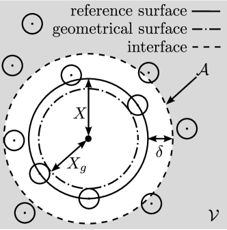
Figure 1: The reference surface (solid line) at position $X$ is determined by the external potential. It consists of the set of all reachable locations of the centers of the fluid particles which are closest to the geometrical wall surface (dash-dotted line) at position $X_{g}$. Depending on the wall-fluid interaction potential, the geometrical wall surface and the reference surface can be distinct. The interface of area $\mathcal{A}$ (dashed line) — with respect to which the interfacial tension $\gamma$ in Eq. (16) is defined — may differ from the reference surface. The parameter $\delta$ measures the offset of the interface with respect to the reference surface. This sketch refers to the cases of spherical or cylindrical walls for which $X\equiv R$. However, the concept involving the parameter $\delta$ is valid also for other geometries, in particular for a planar wall with $X\equiv z=0$. If the dashed line runs within the interior of the reference surface, $\delta$ is taken to be negative. The fluid volume $\mathcal{V}$, which refers to the set of all points being not closer to the geometrical wall surface than the interface, is shaded in grey.

III Discussion

The interfacial tension $\gamma$ is defined by

$$L^{2}\beta\gamma=\frac{\beta\Omega_{\text{eq}}-\beta\Omega_{\text{eq}}^{\text{bulk}}}{\mathcal{A}L^{-2}}=\frac{\beta\Omega_{\text{eq}}+\beta p\;\mathcal{V}}{\mathcal{A}L^{-2}}$$ (14)

as the work $\Omega_{\text{eq}}-\Omega_{\text{eq}}^{\text{bulk}}$ per interfacial area $\mathcal{A}$ required to create the interface Rowlinson2002 . On the right hand side of Eq. (14) the relation

$$\beta\Omega_{\text{eq}}^{\text{bulk}}=-\beta p\;\mathcal{V}$$ (15)

between the grand canonical potential $\Omega_{\text{eq}}^{\text{bulk}}$, the fluid volume $\mathcal{V}$, and the bulk pressure $p$ has been used Rowlinson2002 .

The wall-fluid interfacial tension $\gamma$ is not an observable because according to Eq. (14) its value depends — via $\mathcal{V}$ and $\mathcal{A}$ — on the arbitrary choice of an interface position. In order to characterize various interface conventions we introduce a parameter $\delta$ which measures the offset of a chosen interface position with respect to the reference surface (see Fig. 1). In addition to the interfacial area $\mathcal{A}$ the choice of an interface position also determines what is called the fluid volume $\mathcal{V}$, which refers to the set of all points being not closer to the geometrical wall surface than the interface. As a consequence $\mathcal{A}$ and $\mathcal{V}$ are functions of $X+\delta$ where $X$ characterizes the reference surface (see Fig. 1). On the other hand $\Omega_{\text{eq}}$ depends on $X$ only, because due to Eq. (13) only the parameters of the substrate potential (i.e., $X$) enter $\Omega_{\text{eq}}$. Accordingly, one has

$$L^{2}\beta\gamma(X,\delta)=\frac{\beta\Omega_{\text{eq}}(X)+\beta p\;\mathcal{V}(X+\delta)}{\mathcal{A}(X+\delta)L^{-2}}.$$ (16)

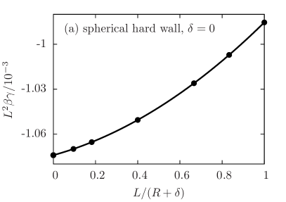
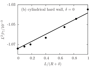
Figure 2: The interfacial tension $\gamma$ of hard spheres with diameter $L$ for the convention $\delta/L=0$ as a function of the radius $R$ of the reference surface forming the boundary of a spherical (a) and a cylindrical (b) hard body. Polynomials (lines) as predicted by morphometric thermodynamics (up to order $1/(R+\delta)^{2}$ for spherical walls and up to order $1/(R+\delta)$ for cylindrical walls) have been fitted to the numerical data (dots). In panel (a) the fit shows good agreement with the data, whereas panel (b) clearly shows deviations from the predicted behavior. This means that for the cylindrical wall the curvature expansion of $\gamma$ Eq. (3) does not terminate after the first-order term, in contradiction to the prediction from morphometric thermodynamics. The hard spheres interact among each other via the square-shoulder potential $U(r)$ in Eq. (4) with $\beta U_{0}=\infty$. The chemical potential is chosen as $\beta\mu=-2.768839$ which corresponds to the low packing fraction $\eta=\frac{\pi}{6}\varrho_{\text{eq}}^{\text{bulk}}L^{3}\approx 0.02656$.

Our data are calculated within the convention $\delta/L=0$ as this choice is convenient for various types of interactions $U$. Moreover, in certain studies (see, e.g., Ref. Henderson2002 ) this choice has been argued to be “the natural one from the point of view of statistical mechanics”. Figure 2 shows the interfacial tension $\gamma$ for hard spheres in contact with spherical (Fig. 2(a)) and cylindrical (Fig. 2(b)) walls with various radii $R$ of the reference surface. The packing fraction $\eta=\pi\varrho_{\text{eq}}^{\text{bulk}}L^{3}/6$ is chosen sufficiently small such that the second virial approximation is valid. The plot for the cylindrical walls (Fig. 2(b)) reveals a non-linear increase, similar to the case of spherical walls (Fig. 2(a)). This means that the curvature expansion of $\gamma$ in terms of powers of $1/R$ does not terminate after the first-order term, in contradiction to the prediction from morphometric thermodynamics for cylindrical walls.

Evaluating Eq. (16) for $\delta=0$ and arbitrary $\delta\neq 0$ and exploiting that $\Omega_{\text{eq}}$ does not depend on $\delta$ leads to

$$\begin{aligned} L^{2}\beta\gamma(X,\delta)=&\frac{\mathcal{A}(X)}{\mathcal{A}(X+\delta)}L^{2}\beta\gamma(X,\delta=0)\\ &+\frac{L^{2}\beta p}{\mathcal{A}(X+\delta)}\left(\mathcal{V}(X+\delta)-\mathcal{V}(X)\right).\end{aligned}$$ (17)

According to Eq. (17) the interfacial tension $\gamma(X,\delta=0)$ calculated for the convention $\delta/L=0$ can be translated to that for any other choice of the convention. For example the convention $\delta/L=-0.5$ is often used when discussing hard spheres confined by hard walls because this choice renders the interface to coincide with the geometrical wall surface at position $X_{g}$ in Fig. 1, which, in this case, is separated from the reference surface at position $X$ in Fig. 1 by a distance given by the particle radius $L/2$.

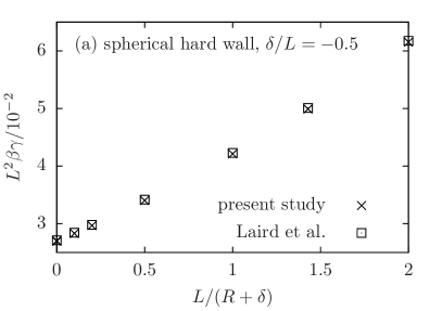
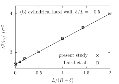
Figure 3: Comparison of the simulation results of Laird et al. Laird2012 (squares $\Box$) with the corresponding data of the present DFT study (crosses $\times$) for the packing fraction $\eta\approx 0.02656$. The latter have been obtained by translating the data displayed in Fig. 2 (for $\delta=0$) into the convention $\delta/L=-0.5$ by using Eq. (17). In contrast to Fig. 2(b), the plot of the interfacial tension in the case of a cylindrical wall (b) almost coincides with a straight line.

In Fig. 3 simulation results of Laird et al. Laird2012 for hard spheres with packing fraction $\eta=0.02656$, obtained for $\delta/L=-0.5$, are plotted together with the data of Fig. 2 which have been translated into the convention $\delta/L=-0.5$ according to Eq. (17). The agreement with the simulation data is very good. In particular, within this convention for $\delta$, in the case of a cylindrical wall (Fig. 3(b)) the data points almost coincide with a straight line, in accordance with the prediction of morphometric thermodynamics. This finding has also been confirmed for the packing fractions $\eta\approx 0.053$ and $0.101$, for which the respective plots are qualitatively similar to those in Fig. 3 except that, as expected, the results of the present virial expansion deviate more and more from the simulation data upon increasing the density.

Figures 2 and 3, which are based on the same microscopic system, show that the interfacial tension depends strongly on the choice of the convention for $\delta$. Upon varying $\delta$ not only the sign of $\gamma$ may change, as already noted in Ref. Bryk2003 , but also the magnitude and even the qualitative functional form, which is revealed clearly in the case of cylindrical walls.

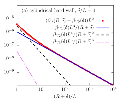
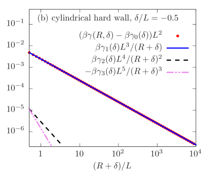
Figure 4: Dependence of the interfacial tension $\gamma$ for hard spheres at a cylindrical hard wall on the radius $R$ of the reference surface and on the shift parameter $\delta$. The contribution of the planar wall $\gamma_{0}(\delta)$, which corresponds to the limit $R\rightarrow\infty$, has been subtracted. The numerical data (red dots) are obtained within the convention $\delta/L=0$ (a) and translated to the convention $\delta/L=-0.5$ (b) via Eq. (17). The three straight lines represent the terms $n=1,2,3$ of the curvature expansion in Eq. (18). In the case $\delta/L=0$ the coefficient $\gamma_{2}(\delta)$ is the largest one, i.e., for small $R$ the contribution $\beta\gamma_{2}(\delta)L^{4}/(R+\delta)^{2}$ is the dominant one so that a deviation from the leading behavior $\sim 1/(R+\delta)$ becomes obvious for $R/L\lesssim 3$. Within the convention $\delta/L=-0.5$ the leading coefficient $\gamma_{1}(\delta)$ is the largest one, i.e., the leading term $\beta\gamma_{1}(\delta)L^{3}/(R+\delta)$ is the dominant one. Here $U(r)$ is given by Eq. (4) with $U_{0}\rightarrow\infty$ and $\beta\mu=-3.88$ so that $\eta\approx 0.01$. Note that at $(R+\delta)/L=1$ the plots render the values of the dimensionless coefficients $\beta\gamma_{n}(\delta)L^{2}$.

Figure 4 shows the behavior of the same microscopic system as above (hard spheres exposed to a hard cylindrical wall) described in terms of two conventions for $\eta\approx 0.01$. The data are presented in log-log plots which facilitate the identification of power laws in $1/(R+\delta)$. In this presentation the contribution $\gamma_{0}(\delta)$ of the planar wall is subtracted so that the plotted quantity vanishes for $R\rightarrow\infty$. Within the convention $\delta/L=0$, at $R\approx 3L$ there is a crossover between two power laws. Thus the dependence of the interfacial tension on $1/R$ consists of more than the leading term $\sim 1/R$ which, according to morphometric thermodynamics, would be the only one allowed for the cylindrical configuration. The behavior is different within the convention $\delta/L=-0.5$. There, within this presentation, the interfacial tension is represented by an almost straight line throughout the whole range of $(R+\delta)/L$ shown. In order to analyze the curvature dependence of the interfacial tension more quantitatively, we assume that $\gamma(R,\delta)$ can be expanded in terms of a power series in $1/(R+\delta)$:

$$L^{2}\beta\gamma(R,\delta)=L^{2}\sum\limits_{n=0}^{\infty}L^{n}\frac{\beta\gamma_{n}(\delta)}{(R+\delta)^{n}}.$$ (18)

For various radii $R$ of the reference surface of the curved wall, the interfacial tension $\gamma$ is calculated numerically (red dots in Fig. 4) and fitted to the curvature expansion Eq. (18) with $n\leq 10$. This way the coefficients $\gamma_{n}(\delta)$ have been determined. Only the coefficient $\gamma_{0}(\delta)$, which is the interfacial tension at a planar wall, can be obtained independently without fitting. In Fig. 4 the terms $L^{n+2}\beta\gamma_{n}(\delta)/(R+\delta)^{n}$ corresponding to $n\in\{1,2,3\}$ in the curvature expansion of Eq. (18) are plotted as lines. Within the convention $\delta/L=0$ the quadratic coefficient $\gamma_{2}$, which vanishes within morphometric thermodynamics, is even larger than the linear coefficient $\gamma_{1}$; this explains the crossover between two power laws describing the numerical data (red dots). However, within the convention $\delta/L=-0.5$ the first-order coefficient $\gamma_{1}$ is much larger than the higher order coefficients $\gamma_{n},n\geq 2$, so that in this case morphometric thermodynamics is a very good approximation of the exact curvature dependence of the interfacial tension. Within the class of systems with square-well-like or square-shoulder-like particle-particle interactions, we have studied a large variety of configurations within the convention $\delta/L=0$ in the same way as shown in Fig. 4. Fluids with packing fractions $\eta\in\{0.01,\,0.02,\,0.05,\,0.10\}$ and with interaction strengths $\beta U_{0}\in\{-0.1,0.1,\,1,\,\infty\}$ have been examined near spherical and cylindrical hard walls. In addition to the interfacial tension $\gamma$, the dimensionless excess adsorption $\Gamma$ Rowlinson2002

$$L^{2}\Gamma(X,\delta)=\frac{N(X)-\varrho_{\text{eq}}^{\text{bulk}}\,\mathcal{V}(X+\delta)}{\mathcal{A}(X+\delta)L^{-2}},$$ (19)

has been calculated for $U_{0}>0$ where $N(X)=\int_{\mathcal{V}(X)}d^{3}r\varrho(\mathbf{r})$ denotes the number of fluid particles. Our corresponding observations can be summarized as follows:

• Apart from opposite signs, both the excess adsorption $\Gamma$ and the interfacial tension $\gamma$ exhibit a similar dependence on the radius of curvature $R$.

• The functional form of $L^{2}\left(\beta\gamma(R,0)-\beta\gamma_{0}(0)\right)$ is similar when comparing fluids with the same bulk state near a spherical and a cylindrical hard wall. Because in all considered cases the third order coefficient $\gamma_{3}$ is smaller than $\gamma_{1}$ and $\gamma_{2}$, morphometric thermodynamics turns out to be a better approximation for spherical than for cylindrical walls.

• Decreasing packing fractions $\eta$ or interaction strengths $U_{0}>0$ result in a shift of the crossover between the power laws describing $L^{2}(\gamma(R,0)-\gamma_{0}(0))$ towards larger radii $R$, i.e., the second coefficient $\gamma_{2}$ becomes larger in comparison to the first coefficient $\gamma_{1}$. Apart from that, the behavior of $L^{2}\left(\beta\gamma(R,0)-\beta\gamma_{0}(0)\right)$ is similar to the one shown in Fig. 4. For $U_{0}<0$, $L^{2}\left(\beta\gamma(R,0)-\beta\gamma_{0}(0)\right)$ exhibits a zero because the coefficients $\gamma_{1}$ and $\gamma_{2}$ have opposite signs.

• For some of the above systems the data have been translated to the convention $\delta/L=-0.5$ by using Eq. (17). In these cases, for the spherical wall configurations the third order coefficient $\gamma_{3}$ is much smaller than $\gamma_{1}$ and $\gamma_{2}$, and for the cylindrical wall configurations the leading coefficient $\gamma_{1}$ is much larger than the subleading ones. Therefore, within this convention morphometric thermodynamics turns out to be a very good approximation.

The comparison of the plots in Figs. 4(a) and (b) shows that the coefficients $\gamma_{n}(\delta)$ in the curvature expansion (Eq. (18)) indeed depend on the chosen convention $\delta$. In order to examine the implications of shifting the position of the interface (see Fig. 1) this dependence is investigated more closely. The derivative of Eq. (16) with respect to $\delta$ for fixed $R$ leads to

$$\begin{aligned} L\frac{\partial}{\partial\delta}L^{2}\beta\gamma(R,\delta)&=-L^{3}\beta p-d\frac{L}{R+\delta}L^{2}\beta\gamma(R,\delta)\\ d&=\begin{cases}2,&\text{spherical wall}\\ 1,&\text{cylindrical wall},\end{cases}\end{aligned}$$ (20)

where $\mathcal{V}^{\prime}(R+\delta)=-\mathcal{A}(R+\delta)$ and $\mathcal{A}^{\prime}(R+\delta)/\mathcal{A}(R+\delta)=d/(R+\delta)$ have been used. The derivative of Eq. (18) with respect to $\delta$ gives

$$\begin{aligned} L\frac{\partial}{\partial\delta}L^{2}\beta\gamma(R,\delta)=L^{3}\sum\limits_{n=0}^{\infty}\bigg{\{}&L^{n}\frac{\beta\gamma^{\prime}_{n}(\delta)}{(R+\delta)^{n}}\\ &-L^{n}n\frac{\beta\gamma_{n}(\delta)}{(R+\delta)^{n+1}}\bigg{\}}.\end{aligned}$$ (21)

Equating Eqs. (20) and (21) and using Eq. (18) leads to

$$\begin{aligned} -L^{3}\beta p&=L^{3}\beta\gamma_{0}^{\prime}(\delta)+\sum\limits_{n=1}^{\infty}\frac{L^{n}}{(R+\delta)^{n}}\\ &\times\left\{L^{3}\beta\gamma^{\prime}_{n}(\delta)+(d-n+1)L^{2}\beta\gamma_{n-1}(\delta)\right\}\end{aligned}$$ (22)

for all $R$. Comparison order by order in $(R+\delta)^{-1}$ in Eq. (22) renders

$$O((R+\delta)^{0}):\quad-L^{3}\beta p=L^{3}\beta\gamma^{\prime}_{0}(\delta)$$ (23)

and

$$\begin{aligned} O((R+\delta)^{-n}),n\geq 1:&\\ L^{3}\beta\gamma^{\prime}_{n}(\delta)+&(d-n+1)L^{2}\beta\gamma_{n-1}(\delta)=0.\end{aligned}$$ (24)

Integration of Eqs. (23) and (24) with respect to $\delta$ leads to the following iterative algorithm for determining the dependence of the coefficients $\gamma_{n}(\delta),n\geq 0$, on $\delta$:

$$\begin{aligned} &n=0:\\ &L^{2}\beta\gamma_{0}(\delta)=L^{2}\beta\gamma_{0}(0)-L^{3}\beta p\frac{\delta}{L},\\ &n\geq 1:\\ &L^{2}\beta\gamma_{n}(\delta)=L^{2}\beta\gamma_{n}(0)+(n-d-1)\int\limits_{0}^{\delta}\frac{\text{d}\tilde{\delta}}{L}L^{2}\beta\gamma_{n-1}(\tilde{\delta})\\ &d=\begin{cases}2,&\text{spherical wall}\\ 1,&\text{cylindrical wall}.\end{cases}\end{aligned}$$ (25)

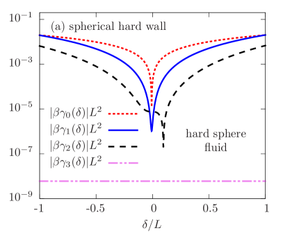
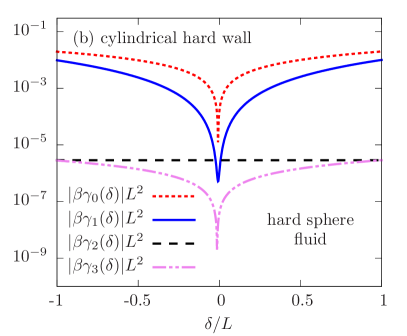
Figure 5: Reduced coefficients $\gamma_{n}(\delta),n\in\{0,1,2,3\},$ characterizing the curvature expansion in Eq. (18) as function of the shift parameter $\delta$ and as obtained from Eq. (25). The data correspond to a hard sphere fluid at $\beta\mu=-3.88$, so that $\eta\approx 0.01$, exposed to hard spherical (a) or cylindrical (b) walls.

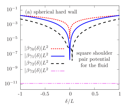
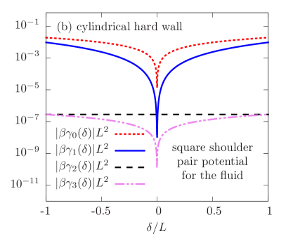
Figure 6: Reduced coefficients $\gamma_{n}(\delta),n\in\{0,1,2,3\},$ characterizing the curvature expansion in Eq. (18) as function of the shift parameter $\delta$ and as obtained from Eq. (25). The data correspond to a fluid with a square-shoulder pair potential $U(r)$ (Eq. (4)) with $\beta U_{0}=0.1$ and $\beta\mu=-3.95$ so that $\eta\approx 0.01$. The fluid is exposed to hard spheres (a) or hard cylinders (b).

The dependence of the coefficients $\gamma_{n}(\delta)$ on $\delta$ is fully determined once in Eq. (25) the values of $\gamma_{n^{\prime}}(0)$ for all $n^{\prime}\leq n$ are known. Here the values $\gamma_{n}(0)$ are obtained by fitting Eq. (18) for $n\leq 10$ to the numerical data within the convention $\delta/L=0$. Considering terms in Eq. (18) to such high orders was necessary in order to achieve a sufficiently high precision for the actually interesting coefficients $\gamma_{1}(\delta),\dots,\gamma_{3}(\delta)$ (see Figs. 4-9); taking the additional terms of order $n\geq 4$ into account guarantees that these coefficients $\gamma_{1}(\delta),\dots,\gamma_{3}(\delta)$ are not affected by the fast-decaying contributions of the full curvature expansion. Thereby we have found that the ratio of the leading coefficients for the spherical wall, $\gamma_{1}^{s}(0)$, and for the cylindrical wall, $\gamma_{1}^{c}(0)$, takes the value $\gamma_{1}^{s}(0)/\gamma_{1}^{c}(0)=2$ for all systems considered here, with a relative deviation of $10^{-7}$ or less. Comparison of that numerical result with the exact relation $\gamma_{1}^{s}(\delta)/\gamma_{1}^{c}(\delta)=2$, which follows from the fact that the total curvatures $J=1/R_{1}+1/R_{2}$ of a sphere, $J^{s}$, and of a cylinder, $J^{c}$, are related by $J^{s}=2J^{c}$ (see Refs. Koenig2004 ; Blokhuis2013 ), validates our numerical approach. Motivated by this relationship between the leading coefficients we have considered also the ratio of the next-to-leading coefficients. For small packing fractions we have obtained $\gamma_{2}^{s}(\delta)/\gamma_{2}^{c}(\delta)\approx 8/3$ for $\delta=0$, independently of the particle-particle interaction potential $U$. The value of this ratio does depend on the convention for $\delta$ because the spherical coefficient $\gamma_{2}^{s}(\delta)$ varies with $\delta$, whereas the cylindrical coefficient $\gamma_{2}^{c}$ is constant (see discussion below). Actually, the value $8/3$ can be obtained from the exact analytical expressions for the surface tension in the low-density limit for a fluid of hard spheres Urrutia2014 . Moreover, the exact expression in Eq. (36) (see Appendix A) describes the deviation of the ratio $\gamma_{2}^{s}(0)/\gamma_{2}^{c}(0)$ from $8/3$ for an ideal gas of particles as function of the strength $\beta V_{p}^{yu}$ of a short-ranged excess external potential in addition to the hard wall potential.

It is interesting to pay special attention to the coefficient $\gamma_{n=d+1}$ in Eq. (25) which is the coefficient of the lowest order being not in accordance with morphometric thermodynamics. For this order $n=d+1$ one has $n-d-1=0$ and therefore $\gamma_{d+1}$ is constant in $\delta$ (see Eq. (25) for $n\geq 1$). This checks with Fig. 4 (corresponding to $d=1$), where the values of the coefficients $\gamma_{2}$ can be read from the lines $\sim 1/(R+\delta)^{2}$ at $(R+\delta)/L=1$. The value of $\gamma_{2}$ is not vanishing and it is the same in both conventions for $\delta$. This implies that within morphometric thermodynamics the curvature expansion is not exact for any convention for $\delta$. On the other hand, if, as a consequence of Eq. (25), the $R$-dependence of $\gamma(R,\delta)$ within morphometric thermodynamics would be exact for any single convention for $\delta$, it would be exact for all conventions for $\delta$. However, this statement is of no practical use, because, on the basis of numerical data, it is virtually impossible to prove that there is a convention for $\delta$ within which the morphometric form of the interfacial tension is exact. In contrast, Fig. 4 shows that even if the non-morphometric coefficients $\gamma_{n}(\delta)$ ($n\geq 2$ for a cylindrical wall) are numerically small for one convention for $\delta$ (see Fig. 4(b)) they may be large for another (see Fig. 4(a)). The reason for this is that the operation of approximating the curvature-dependence of the interfacial tension by the form predicted within morphometric thermodynamics does not commute with the operation of shifting the interface.

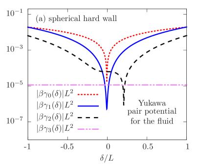
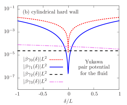
Figure 7: Same as Fig. 6 for a fluid with a Yukawa pair potential (Eq. (5)) with $\beta U_{0}=0.1$, $\beta\mu=-3.94$, and $L_{c}/L=5$ so that $\eta\approx 0.01$.

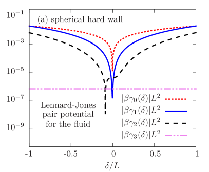
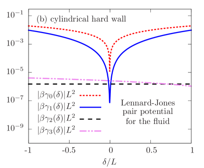
Figure 8: Same as Fig. 7 for a fluid with a Lennard-Jones pair potential (Eq. (6)) with $\beta U_{0}=0.1$, $\beta\mu=-3.92$, and $L_{c}/L=5$ so that $\eta\approx 0.01$.

Figure 5 shows the dependence of the coefficients $\gamma_{n}(\delta)$, $0\leq n\leq 3$, of the curvature expansion Eq. (18) on the shift parameter $\delta$. Except for the first non-morphometric coefficient (i.e., $\gamma_{3}$ for a sphere and $\gamma_{2}$ for a cylinder), which is constant in $\delta$, the coefficients $\gamma_{n}(\delta)$ vary over several orders of magnitude upon changing $\delta$. This is particularly pronounced near $\delta/L=0$, where the morphometrically allowed coefficients are small; in the case of a cylindrical wall $\gamma_{1}$ is even smaller than the leading non-morphometric coefficient $\gamma_{2}$. However, apart from this region around $\delta/L=0$, e.g., at $\delta/L=-0.5$, the morphometrically allowed coefficients exceed the leading non-morphometric coefficient by several orders of magnitude. These observations are in agreement with the findings of Fig. 4 which is based on the same system and where for each convention for $\delta$ the coefficients, the values of which are rendered at $(R+\delta)/L=1$, have been fitted independently. Figure 5 demonstrates that the interfacial tension cannot be represented exactly by the form obtained within morphometric thermodynamics, and that the quality of the approximation of the interfacial tension by the morphometric form depends on the position of the interface parameterized by the shift $\delta$.

So far we have mainly focussed on hard sphere fluids near hard walls. In the following we discuss to which extent the aforementioned observations can be extended to other systems. This will be discussed along the lines of Fig. 5.

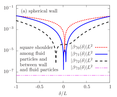
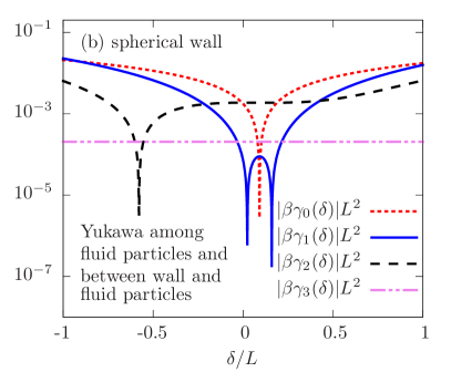
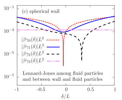
Figure 9: Reduced coefficients $\gamma_{n}(\delta),n\in\{0,1,2,3\},$ characterizing the curvature expansion in Eq. (18) as function of the shift parameter $\delta$ and as obtained from Eq. (25). Panels (a), (b), and (c) belong to the same systems as in Figs. 6(a), 7(a), and 8(a), respectively, with an additional soft part $V$ of the external substrate potential: (a) $V$ given by Eq. (38), (b) $V$ given by Eq. (39), and (c) $V$ given by Eq. (41). The data correspond to the following choice of system parameters: $\beta V_{p}^{sq}=\beta V_{p}^{yu}=\beta V_{p}^{LJ}=0.1$ (see Appendix B), $L_{w}/L=1$, and $L_{cw}/L=5$.

Figure 6 displays the corresponding results for a fluid which is governed by a square-shoulder pair potential of finite strength $\beta U_{0}$, acting as a representative for interaction potentials of finite range. The comparison with Fig. 5 does not reveal qualitative changes. Figures 7 and 8, respectively, display the corresponding results for a fluid with a Yukawa pair potential, representing exponentially decaying interaction potentials, and for a Lennard-Jones pair potential, representing algebraically decaying pair potentials. Although comparing them with Figs. 5 and 6 reveals certain differences, the main conclusions remain the same: the coefficients $\gamma_{n}(\delta)$ are strongly affected by the choice of the convention for $\delta$ and, whereas for none of the systems considered here the curvature-dependence of the interfacial tension is exactly in agreement with morphometric thermodynamics, the morphometric form of the interfacial tension may be an excellent approximation for suitable conventions for $\delta$.

In order to further assess to which extent the above findings are generic, an additional excess part $V$ of the external potential $V^{\text{ext}}$ is considered. This excess part $V$ is obtained by integrating the pair potential $U_{w}(r)$ between a fluid particle and a wall particle over the volume $\tilde{\mathcal{V}}$ of the wall:

$$\beta V(\mathbf{r})=\varrho_{w}\int\limits_{\tilde{\mathcal{V}}}d^{3}r^{\prime}\beta U_{w}(|\mathbf{r}-\mathbf{r^{\prime}}|),$$ (26)

where in $\tilde{\mathcal{V}}$ the number density $\varrho_{w}$ of the wall is taken to be constant. The particle-wall potentials $U_{w}(r)$ are chosen to be of a similar form as the pair potentials $U(r)$ between the fluid particles (Eqs. (4)-(6)), with the exception that the Yukawa-like wall-particle potential is not truncated and the repulsive part of a Lennard-Jones-like wall potential is replaced by a hard wall. The pair potentials are characterized by an energy scale $U_{0w}$, a length scale $L_{w}$ and a cut-off length $L_{cw}$ such that $U_{w}(r>L_{cw})=0$:

• the square-well ($U_{0w}<0$) or square-shoulder ($U_{0w}>0$) potential

  $$\beta U_{w}(r\leq L_{cw})=\beta U_{0w}$$ (27)

  with $L_{w}=L_{cw}$,

• the Yukawa potential ($U_{0w}>0$, $L_{cw}=\infty$)

  $$\beta U_{w}(r)=\beta U_{0w}\frac{L_{w}}{r}\exp\left(-\frac{r}{L_{w}}\right),$$ (28)

• the Lennard-Jones potential ($U_{0w}>0$)

  $$\beta U_{w}(r)=\begin{cases}\beta U_{0w}\left(\left(\frac{L_{w}}{r}\right)^{12}-\left(\frac{L_{w}}{r}\right)^{6}\right)&,L_{w}\leq r\leq L_{cw}\\ \infty&,r<L_{w}.\end{cases}$$ (29)

The resulting excess parts $V$ of the substrate potentials as function of the radial distance $z$ to a spherical reference surface of radius $R$ are given in Eqs. (38), (39), and (41) in Appendix B.

In Fig. 9 the results for systems with a non-vanishing excess part $V$ of the external potential are shown. The parameters are chosen such that, apart from $V\neq 0$, the same systems as in Figs. 6(a), 7(a), and 8(a) are analyzed. It again turns out that the coefficients $\gamma_{n}(\delta)$ exhibit a strong dependence on $\delta$ so that the quality of morphometric thermodynamics as an approximation depends sensitively on the convention for $\delta$. As a general trend, for all three examples shown in Fig. 9 the non-morphometric coefficient $|\beta\gamma_{3}(\delta)|L^{2}$ is not negligible in wider ranges of conventions for $\delta$ than in the cases without an excess substrate potential $V$. In this sense the quality of morphometric thermodynamics as an approximation deteriorates in the presence of excess parts $V$ of the substrate potential.

IV Conclusions and Summary

By using density functional theory within the second virial approximation we have analyzed several model fluids with small number densities in contact with planar, spherical, or cylindrical walls. We have compared the curvature expansion in Eq. (18) of the interfacial tension $\gamma$ with the expression derived within morphometric thermodynamics (Eq. (3)). Particular attention has been paid to the implications of the choice of the position of the interface, which underlies the definition of the interfacial tension (Eq. (16) and Fig. 1). For none of the considered systems the expression for the interfacial tension in accordance with morphometric thermodynamics is exact, regardless of whether the particles interact with each other via a square-well or square-shoulder potential (Eq. (4)), a Yukawa potential (Eq. (5)), or a Lennard-Jones potential (Eq. (6)). As shown in Figs. 5-8 the coefficients $\gamma_{n}(\delta)$ of the curvature expansion in Eq. (18) may depend sensitively on the chosen interface convention, which is expressed in terms of the shift parameter $\delta$ (Fig. 1). There are conventions for which the morphometrically allowed coefficients are much larger than the morphometrically forbidden ones so that within them morphometric thermodynamics is a reliable approximation of the interfacial tension. However, the opposite situation can occur for other interface conventions, in which case morphometric thermodynamics has to be used with caution. In particular the reliability of morphometric thermodynamics as an approximation deteriorates in the presence of excess contributions to the wall potential (Fig. 9). Based on these results, it turns out to be necessary in future applications of morphometric thermodynamics to clearly state which interface convention is chosen and why morphometric thermodynamics is expected to be a reliable approximation for that particular interface convention as compared with others.

Appendix A Ideal Gas

In this appendix we analyze the exactly solvable case of non-interacting particles. The density functional in Eq. (7) with $U(r)=0$ is minimized by the equilibrium number density

$$\begin{aligned} \varrho_{\text{eq}}(\mathbf{r})&=\varrho^{\text{bulk}}_{\text{eq}}\exp\left(-\beta V^{\text{ext}}(\mathbf{r})\right)\quad\text{with}\\ \varrho^{\text{bulk}}_{\text{eq}}&=\Lambda^{-3}\exp(\beta\tilde{\mu}).\end{aligned}$$ (30)

For pointlike ideal gas particles the convention $\delta=0$ is convenient and will be used throughout this appendix. For this choice the interface of area $\mathcal{A}$, the reference surface, and the geometrical wall surface are the same and the interfacial tension $\gamma$ is given by

$$\beta\gamma=-\frac{\varrho^{\text{bulk}}_{\text{eq}}}{\mathcal{A}}\int_{\mathcal{V}}\text{d}^{3}r\left(\exp(-\beta V(\mathbf{r}))-1\right),\delta=0.$$ (31)

The integration volume $\mathcal{V}$ in Eq. (31) equals the volume accessible to the fluid particles. Therefore the integrand depends only on the excess part $V$ of the external potential $V^{\text{ext}}$ (see Eqs. (10) and (11)).
In the case of a hard wall with $V=0$ the interfacial tension of the ideal gas is zero, $\gamma=0$, irrespective of the shape of the wall. Therefore the ideal gas is a useful choice for studying the influence of the excess part $V\neq 0$ of an external potential on the morphometric coefficients.
Here we analyze a Yukawa-like interaction $U_{w}$ (Eq. (28)) between the fluid particles and the wall particles. The excess part $V$ follows from Eq. (26). For planar, spherical, and cylindrical walls, respectively, one finds

$$\begin{aligned} \frac{V(z)}{V_{p}^{yu}}=&\exp\left(-\frac{z}{L_{w}}\right),\quad\text{plane},\\ \frac{V(r)}{V_{p}^{yu}}=&\frac{L_{w}}{r}\exp\left(-\frac{r}{L_{w}}\right)\\ &\times\left[(S-1)\text{e}^{S}+(S+1)\text{e}^{-S}\right],\quad\text{sphere},\\ \frac{V(r)}{V_{p}^{yu}}=&2SI_{1}(S)K_{0}\left(\frac{r}{L_{w}}\right),\quad\text{cylinder},\end{aligned}$$ (32)

where $V_{p}^{yu}=2\pi\varrho_{w}U_{0w}L_{w}^{3}$ denotes the strength of the excess part $V$ at contact with a planar wall and $S=R/L_{w}$ with $K_{0}$ and $I_{1}$ as familiar modified Bessel functions. The expressions in Eq. (32) for the excess parts $V$ of the external potential facilitate to determine exactly the coefficients $\gamma_{n}$ of the curvature expansion of the interfacial tension $\gamma$ in Eq. (31). In the case of a spherical wall we obtain

$$\begin{aligned} \beta\gamma=-\varrho_{\text{eq}}^{\text{bulk}}L_{w}\sum\limits_{n=1}^{\infty}\frac{(-\beta V_{p}^{yu})^{n}}{n!\,n}\bigg{\{}1+\frac{L_{w}}{R}\left[\frac{2}{n}-1-n\right]\\ +\frac{L_{w}^{2}}{R^{2}}\left[\frac{n^{2}}{2}+\frac{n}{2}-1-\frac{3}{n}+\frac{2}{n^{2}}\right]\\ -\frac{L_{w}^{3}}{R^{3}}(2-n)(1-n)\left[\frac{1}{n^{2}}+\frac{1}{n}+\frac{1}{2}+\frac{n}{6}\right]\\ +O\left(\frac{L_{w}^{4}}{R^{4}}\right)\bigg{\}}+O\left(\exp\left(-2\frac{R}{L_{w}}\right)\right),\delta=0,\end{aligned}$$ (33)

and for the cylindrical wall the corresponding result is given by

$$\begin{aligned} \beta\gamma=-\varrho_{\text{eq}}^{\text{bulk}}L_{w}\sum\limits_{n=1}^{\infty}\frac{(-\beta V_{p}^{yu})^{n}}{n!\,n}\bigg{\{}1+\frac{L_{w}}{R}\left[\frac{1}{n}-\frac{1}{2}-\frac{n}{2}\right]\\ +\frac{L_{w}^{2}}{R^{2}}\left[-\frac{1}{2n}-\frac{1}{8}+\frac{n}{8}+\frac{n^{2}}{8}\right]+O\left(\frac{L_{w}^{3}}{R^{3}}\right)\bigg{\}},\delta=0.\end{aligned}$$ (34)

The expression for the planar wall is included in the expressions for the curved walls (Eqs. (33) and (34)) as the term being independent of the radius $R$.
In Eqs. (33) and (34) the respective curvature expansions are presented up to and including the leading non-morphometric coefficients (belonging to $R^{-3}$ in the case of spherical walls and to $R^{-2}$ in the case of cylindrical walls) which in general are non-zero.
Further interesting insight can be gained by studying ratios of particular coefficients:

• The ratio of the leading coefficients $\gamma_{1}$ (belonging to $R^{-1}$),

  $$\frac{\gamma_{1}^{s}}{\gamma_{1}^{c}}=2,$$ (35)

  i.e., a constant value independent of the strength $\beta V_{p}^{yu}$ of the external potential.

• For small amplitudes $\beta V_{p}^{yu}$ the ratio of the subdominant coefficients $\gamma_{2}$ (belonging to $R^{-2}$) is given by

  $$\frac{\gamma_{2}^{s}}{\gamma_{2}^{c}}=\frac{8}{3}\left(1-\frac{1}{18}\left(\beta V_{p}^{yu}\right)^{2}+O\left(\left(\beta V_{p}^{yu}\right)^{3}\right)\right).$$ (36)

  For $\beta V_{p}^{yu}\ll 1$ this ratio reduces to the constant value $8/3$ which has also been found in Ref. Urrutia2014 and in the numerical calculations of Sec. III.

• When comparing the leading ($\gamma_{1}^{c}$) and the subdominant ($\gamma_{2}^{c}$) coefficients for cylindrical walls we obtain

  $$\frac{\gamma_{1}^{c}}{\gamma_{2}^{c}}=-\frac{2}{3}\beta V_{p}^{yu}+\frac{67}{162}\left(\beta V_{p}^{yu}\right)^{2}+O\left(\left(\beta V_{p}^{yu}\right)^{3}\right).$$ (37)

  This implies that for $\beta V_{p}^{yu}\ll 1$ one has $|\gamma_{2}^{c}|\gg|\gamma_{1}^{c}|$ which contradicts the morphometric prediction according to which $\gamma_{2}^{c}$ should be zero.

These results for an ideal gas of non-interacting particles invalidate morphometric thermodynamics if there is a non-vanishing excess part $\beta V_{p}^{yu}\neq 0$ of the external potential.

Appendix B Excess parts of the external potentials

The calculation of the excess parts $V$ of the external potentials according to Eq. (26) results in lengthy expressions. Here these are presented for spherical walls as function of the distance $z\geq 0$ from the reference surface of radius $R$, i.e., the distance from the center of the spherical wall is $r=R+z$.
In the case of the square-well or square-shoulder potential (Eq. (27)) the excess part $V$ of the external potential is given by

$$\begin{aligned} \beta V(z\geq 0)&=\beta V_{p}^{sq}\times\begin{cases}z\geq L_{w}:&0\\ z\leq L_{w}-2R:&2\frac{R^{3}}{L_{w}^{3}}\\ L_{w}-2R<z<L_{w}:&\frac{1}{8}\frac{L_{w}^{3}}{(R+z)^{3}}\bigg{[}\frac{z^{6}}{L_{w}^{6}}+6\frac{z^{5}R}{L_{w}^{6}}+\frac{z^{4}}{L_{w}^{4}}\left(9\frac{R^{2}}{L_{w}^{2}}-6\right)\\ &+\frac{z^{3}}{L_{w}^{3}}\left(4\frac{R^{3}}{L_{w}^{3}}-24\frac{R}{L_{w}}+8\right)+\frac{z^{2}}{L_{w}^{2}}\left(-30\frac{R^{2}}{L_{w}^{2}}+24\frac{R}{L_{w}}-3\right)\\ &+\frac{z}{L_{w}}\left(-12\frac{R^{3}}{L_{w}^{3}}+24\frac{R^{2}}{L_{w}^{2}}-6\frac{R}{L_{w}}\right)+8\frac{R^{3}}{L_{w}^{3}}-3\frac{R^{2}}{L_{w}^{2}}\bigg{]},\end{cases}\\ \beta V_{p}^{sq}&=\frac{2}{3}\pi L_{w}^{3}\beta U_{0w}\varrho_{w}.\end{aligned}$$ (38)

In the case of the Yukawa potential (Eq. (28)) the excess part $V$ is given by

$$\begin{aligned} \beta V(z\geq 0)=&\beta V_{p}^{yu}\exp\left(-\frac{z}{L_{w}}\right)\frac{L_{w}}{R+z}\left(\frac{R}{L_{w}}-1+\exp\left(-\frac{2R}{L_{w}}\right)\left(\frac{R}{L_{w}}+1\right)\right),\\ \beta V_{p}^{yu}=&2\pi\varrho_{w}\beta U_{0w}L_{w}^{3}.\end{aligned}$$ (39)

(Note that Eq. (39) and the sphere expression in Eq. (32) are identical.)
In the case of the Lennard-Jones-like potential (Eq. (29)) the reference surface and the geometrical wall surface do not coincide: $R=R_{g}+L_{w}$ with $R_{g}$ denoting the radius of the geometrical wall. Integration according to Eq. (26) results in an expression $\beta V_{g}(z_{g},R_{g})$ in which $z_{g}$ measures the distance from the geometrical wall surface, i.e., the distance from the center of the spherical wall is $r=R_{g}+z_{g}$:

$$\beta V_{g}(z_{g},R_{g})= \beta V_{p}^{LJ}\frac{\mathcal{I}_{12}(z_{g},R_{g})-\mathcal{I}_{6}(z_{g},R_{g})}{-2\pi L_{w}^{3}\left\{-\frac{1}{10}\left(\frac{10}{9}\frac{L_{w}^{9}}{L_{cw}^{9}}-\frac{L_{w}^{10}}{L_{cw}^{10}}-\frac{1}{9}\right)+\frac{1}{4}\left(\frac{4}{3}\frac{L_{w}^{3}}{L_{cw}^{3}}-\frac{L_{w}^{4}}{L_{cw}^{4}}-\frac{1}{3}\right)\right\}},$$

$$\beta V_{p}^{LJ}= -2\pi L_{w}^{3}\varrho_{w}\beta U_{0w}\left\{-\frac{1}{10}\left(\frac{10}{9}\frac{L_{w}^{9}}{L_{cw}^{9}}-\frac{L_{w}^{10}}{L_{cw}^{10}}-\frac{1}{9}\right)+\frac{1}{4}\left(\frac{4}{3}\frac{L_{w}^{3}}{L_{cw}^{3}}-\frac{L_{w}^{4}}{L_{cw}^{4}}-\frac{1}{3}\right)\right\},$$

$$\mathcal{I}_{n}(z_{g},R_{g})= \frac{2\pi}{n-2}L_{w}^{n-1}\frac{L_{w}}{R_{g}+z_{g}}\sum_{j=1}^{5}A_{j}^{(n)}(z_{g},R_{g}),$$

$$A_{1}^{(n)}(z_{g},R_{g})= L_{w}^{4-n}\Bigg{\{}\frac{1}{n-3}\frac{R_{g}}{L_{w}}\left(\frac{z_{g}^{3-n}}{L_{w}^{3-n}}+\frac{(2R_{g}+z_{g})^{3-n}}{L_{w}^{3-n}}\right)$$

$$+\frac{1}{(n-3)(n-4)}\left(-\frac{z_{g}^{4-n}}{L_{w}^{4-n}}+\frac{(2R_{g}+z_{g})^{4-n}}{L_{w}^{4-n}}\right)\Bigg{\}},$$

$$A_{2}^{(n)}(z_{g},R_{g})= L_{w}^{4-n}\Theta\left(R_{g}+z_{g}-L_{cw}\right)\Bigg{\{}\frac{1}{3-n}\frac{R_{g}}{L_{w}}\frac{(2R_{g}+z_{g})^{3-n}}{L_{w}^{3-n}}-\frac{1}{2}\frac{L_{cw}^{2-n}}{L_{w}^{2-n}}\frac{R_{g}^{2}}{L_{w}^{2}}$$

$$-\frac{1}{(4-n)(3-n)}\left(\frac{(2R_{g}+z_{g})^{4-n}}{L_{w}^{4-n}}-\frac{(R_{g}+z_{g})^{4-n}}{L_{w}^{4-n}}\right)\Bigg{\}},$$

$$A_{3}^{(n)}(z_{g},R_{g})= L_{w}^{4-n}\Theta(2R_{g}+z_{g}-L_{cw})\Theta(L_{cw}-R_{g}-z_{g})\Bigg{\{}\frac{1}{3-n}\frac{R_{g}}{L_{w}}\frac{(2R_{g}+z_{g})^{3-n}}{L_{w}^{3-n}}$$

$$-\frac{1}{2}\frac{L_{cw}^{2-n}}{L_{w}^{2-n}}\frac{R_{g}^{2}}{L_{w}^{2}}-\frac{1}{3-n}\frac{L_{cw}^{3-n}}{L_{w}^{3-n}}\frac{L_{cw}-R_{g}-z_{g}}{L_{w}}$$

$$+\frac{1}{2}\frac{L_{cw}^{2-n}}{L_{w}^{2-n}}\frac{(L_{cw}-R_{g}-z_{g})^{2}}{L_{w}^{2}}+\frac{L_{cw}^{4-n}-(2R_{g}+z_{g})^{4-n}}{(3-n)(4-n)L_{w}^{4-n}}\Bigg{\}},$$

$$A_{4}^{(n)}(z_{g},R_{g})= L_{w}^{4-n}\Theta(z_{g}-L_{cw})\Bigg{\{}\frac{1}{3-n}\frac{R_{g}}{L_{w}}\frac{z_{g}^{3-n}}{L_{w}^{3-n}}+\frac{1}{2}\frac{L_{cw}^{2-n}}{L_{w}^{2-n}}\frac{R_{g}^{2}}{L_{w}^{2}}+\frac{z_{g}^{4-n}-(R_{g}+z_{g})^{4-n}}{(4-n)(3-n)L_{w}^{4-n}}\Bigg{\}},$$

$$A_{5}^{(n)}(z_{g},R_{g})= L_{w}^{4-n}\Theta(R_{g}+z_{g}-L_{cw})\Theta(L_{cw}-z_{g})\Bigg{\{}\frac{1}{3-n}\frac{L_{cw}^{3-n}}{L_{w}^{3-n}}\frac{R_{g}+z_{g}-L_{cw}}{L_{w}}$$

$$+\frac{1}{2}\frac{L_{cw}^{2-n}}{L_{w}^{2-n}}\frac{(R_{g}+z_{g}-L_{cw})^{2}}{L_{w}^{2}}+\frac{L_{cw}^{4-n}-(R_{g}+z_{g})^{4-n}}{(4-n)(3-n)L_{w}^{4-n}}\Bigg{\}}.$$ (40)

The excess part $V$ of the external potential as function of the distance $z$ from the reference surface of radius $R$ is related to $V_{g}$ in Eq. (40) via

$$\beta V(z\geq 0)=\beta V_{g}(z+L_{w},R-L_{w}).$$ (41)

References

• (1) P.-M. König, R. Roth, and K. R. Mecke, Phys. Rev. Lett. 93, 160601 (2004).
• (2) R. Roth, Y. Harano, and M. Kinoshita, Phys. Rev. Lett. 97, 078101 (2006).
• (3) H. Hansen-Goos, R. Roth, K. Mecke, and S. Dietrich, Phys. Rev. Lett. 99, 128101 (2007).
• (4) B. B. Laird, A. Hunter, and R. L. Davidchack, Phys. Rev. E 86, 060602(R) (2012).
• (5) M. E. Evans and R. Roth, Phys. Rev. Lett. 112, 038102 (2014).
• (6) H. Hadwiger, Vorlesungen über Inhalt, Oberfläche und Isoperimetrie (Springer, Berlin, 1957).
• (7) K. R. Mecke, Int. J. Mod. Phys. B 12, 861 (1998).
• (8) P. Bryk, R. Roth, K. R. Mecke, and S. Dietrich, Phys. Rev. E 68, 031602 (2003).
• (9) B. Groh and S. Dietrich, Phys. Rev. E 59, 4216 (1999).
• (10) E. M. Blokhuis, Phys. Rev. E 87, 022401 (2013).
• (11) I. Urrutia, Phys. Rev. E 89, 032122 (2014).
• (12) H. Hansen-Goos, J. Chem. Phys. 141, 171101 (2014).
• (13) R. Evans, Adv. Phys. 28, 143 (1979).
• (14) J. P. Hansen and I. R. McDonald, Theory of Simple Liquids (Academic, London, 1976).
• (15) M. Schmidt, H. Löwen, J. M. Brader, and R. Evans, J. Phys. Condens. Matt. 14, 9353 (2002).
• (16) J. S. Rowlinson and B. Widom, Molecular Theory of Capillarity (Dover Publications, New York, 2002).
• (17) J. R. Henderson, J. Chem. Phys. 116, 5039 (2002).