Electrostatic potential variation on the flux surface and its impact on impurity transport

Abstract

The particle transport of impurities in magnetically confined plasmas under some conditions does not find, neither quantitatively nor qualitatively, a satisfactory theory-based explanation. This compromise the successful realization of thermo-nuclear fusion for energy production since its accumulation is known to be one of the causes that leads to the plasma breakdown.
In standard reactor-relevant conditions this accumulation is in most stellarators intrinsic to the lack of toroidal symmetry, that leads to the neoclassical electric field to point radially inwards. This statement, that the standard theory allows to formulate, has been contradicted by some experiments that showed weaker or no accumulation under such conditions [1, 2].
The charge state of the impurities makes its transport more sensitive to the electric fields. Thus, the short length scale turbulent electrostatic potential or its long wave-length variation on the flux surface $\Phi_{1}$ – that the standard neoclassical approach usually neglects – might possibly shed some light on the experimental findings. In the present work the focus is put on the second of the two, and investigate its influence of the radial transport of C⁶⁺. We show that in LHD it is strongly modified by $\Phi_{1}$, both resulting in mitigated/enhanced accumulation at internal/external radial positions; for Wendelstein 7-X, on the contrary, $\Phi_{1}$ is expected to be considerably smaller and the transport of C⁶⁺ not affected up to an appreciable extent; and in TJ-II the potential shows a moderate impact despite of the large amplitude of $\Phi_{1}$ for the parameters considered.

1 Introduction

From a passive viewpoint the presence of impurities in thermo-nuclear fusion plasmas is intrinsic and is bound to the main wall material, whose choice in turn depends on the desired wall recycling properties. Furthermore the deliberate introduction of certain impurity species is widely recognized as a powerful technique for the reduction of the heat exhaust on the plasma facing components to an tolerable level (see e.g. [3] and reference therein). The high radiative efficiency of impurities, exploited for that purpose, results at the same time in a disadvantage if they accumulate in the plasma core – that apart from diluting the fusion fuel – in some cases can lead to the radiative collapse of the plasma. The balance between the required concentration in the edge region and the lack of its accumulation in the core undoubtedly needs of the identification of the physical mechanisms that determine the radial particle flux of impurities, leading them to accumulate or to avoid or mitigate that accumulation.
To that respect, in stellarators and heliotrons the standard physical picture can be summarized as follows. The lack of toroidal symmetry of the magnetic field structure in these devices leads to the existence of a population of particles trapped in the helical wells that determines the fluxes. Unless that the magnetic field is such that the net radial drift of these particles is sufficiently reduced, the total flux surface average radial current does not vanish. In standard conditions where the bulk ions and electrons with masses $m_{i}$ and $m_{e}$ have similar temperature $T_{i}\sim T_{e}$ their particle diffusion coefficients are such that $D_{i}\sim\sqrt{m_{i}/m_{e}}D_{e}$ [4]. The system needs then of a radial electric field, so-called ambipolar, that reduces the ion radial particle flux to the order of that for the electrons. This reduction is driven by the confining role that the $E\times B$ poloidal precession related to it has on the bulk ions. Tipically the electron confinement is not affected to the same extent due to the more frequent collisions they undergo ($\nu_{e}\sim\sqrt{m_{i}/m_{e}}\nu_{i}$), which prevent them from completing their poloidal precession orbits.
Writing the ambipolar electric field as $\mathbf{E}_{r}=E_{r}\nabla r$, with $E_{r}=-\text{d}\Phi_{0}/\text{d}r$ and $\Phi_{0}=\Phi_{0}(r)$ the electrostatic potential depending by definition only on the flux surface label $r$, it is generally the case that under the previous conditions $E_{r}<0$ (ion root regime), or in other words that the ambipolar electric field points radially inwards. The importance of this for the accumulation of impurities is clear on the context of the standard neoclassical theory.

The particle flux density across the flux surfaces for the species $\alpha$ can be expressed in terms of the neoclassical transport coefficients $L_{ij}^{\alpha}$ and the thermodynamic forces as follows, see e.g. ref. [5],

$$\left<\boldsymbol{\Gamma}_{\alpha}\cdot\nabla r\right>=-n_{s}L_{11}^{s}\left[\frac{n^{\prime}_{\alpha}}{n_{\alpha}}-\frac{Z_{\alpha}eE_{r}}{T_{\alpha}}+\left(\frac{L_{12}^{\alpha}}{L_{11}^{\alpha}}-\frac{3}{2}\right)\frac{T^{\prime}_{\alpha}}{T_{\alpha}}\right].$$ (1)

In eq. (1), $\alpha$ is the species index, $n$ is the particle density, $T$ the temperature, $q$ and $Z$ are respectively the charge and charge state of the species, $e$ is the unit charge modulus and the prime represents the derivative respect to $r$. Therefore it is straightforward to conclude that $E_{r}<0$ drives particles towards the center of the plasma and out of it otherwise. The weight of the charge of the species $Z$ leads inevitably to the dominance of the term driving transport through $E_{r}$ as the $Z$ increases, and subsequently supports a stronger accumulation of impurities as the ionization state of these is higher. In a tokamak the accumulation can be moderated by the so-called temperature screening. This mechanism rests on the fact that the term preceding the temperature gradient in eq. (1) can be negative for ions in the long mean free path regime (lmfp). Subsequently for peaked temperature profiles the inwards flux of bulk ions driven by $T^{\prime}$ enforces the outwards flux of impurities in order to preserve quasi-neutrality along the radial direction. Nevertheless this mechanism cannot take place in stellarators since the asymptotic scaling of the transport coefficients with the collisionality, inversely proportional to $\nu$ and $\sqrt{\nu}$ in the lmfp, is such that $L_{12}^{\alpha}/L_{11}^{\alpha}-3/2>0$ in both cases. Thus the standard prediction for the radial particle transport of impurities in non-axisymmetric devices is roughly speaking of accumulation in ion root regime and absence of it in electron root plasmas [6] where $E_{r}>0$.
Nevertheless, the standard neoclassical picture considering only the ambipolar electrostatic potential $\Phi_{0}$ as constant on each flux surface is particularly questionable in non-axisymmetric systems if impurities of moderate to high charge are considered. This is due to two reasons: 1) regarding the approximation of the full electrostatic potential to only the ambipolar part $\Phi_{0}$ dismisses a potential variation on the flux surface $\Phi_{1}$ that in non-axisymmetric system can be particularly large. This is due to the different dependency of $f_{1}$ (first order departure of the distribution function from its equilibrium $f_{0}$) with the collision frequency than that given in axi-symmetric system, and subsequently the perturbed linear density $n_{1}$ and related charge density and potential; 2) the fact that the weight of the $E\times B$ drift and streaming acceleration related to $\Phi_{1}$ respect to the magnetic drift and mirror acceleration scale proportionally to the charge state $Z$.

Regarding the first of the aforementioned causes, in an axi-symmetric tokamak the effect of the radial electric field is weak and the $E_{r}\times B$ drift is negligible at zeroth order in the normalized Larmor radius to the system size drift kinetic expansion parameter: $\rho_{*}=\rho/L$. Considering a Fourier-Legendre expansion of $f_{1}$ – Fourier in the poloidal coordinate $\theta$ and Legendre in the pitch angle variable $\xi=v_{\|}/v$ – the first order drift kinetic equation (DKE) shows that the structure of $f_{1}$ is such that the only non-zero Legendre coefficients are the even ones for the $\cos(m\theta)$ terms and the odd for the $\sin(m\theta)$ terms. The latter results in addition proportional to the collision frequency. Thus the only terms that can drive a density, and subsequently potential variation on the flux surface formally tend to zero in the limit of vanishing collisionality and will have a $\sin(m\theta)$ components only. Here $m$ is the Fourier poloidal mode number, $v_{\|}$ is the parallel velocity and $v$ is the velocity modulus.
On the other hand the requirement of keeping the $E_{r}\times B$ drift at lowest order particle trajectory in non-axisymmetric systems breaks that structure in $f_{1}$. In this case the bounce averaged solution of the DKE $\left<f_{1}\right>_{b}$ results in a $\cos\theta$ structure with amplitude scaling with $v_{d}/\Omega_{E}$. With $v_{d}$ the modulus of the magnetic drift velocity and $\Omega_{E}=E_{r}/rB_{0}$ the poloidal $E_{r}\times B$ precession frequency. This picture where a finite non-vanishing variation is expected finds a cartoon in the fact that in non-axisymmetric system the helically trapped particles shift their poloidal precession orbits from the birth flux surface due to the action of both the magnetic drift $\mathbf{v}_{d}$ and the poloidal $E_{r}\times B$ drift $\mathbf{v}_{E0}$ [4]. These drift velocities are expressed by

$$\mathbf{v}_{E0}=-\frac{\nabla\Phi_{0}\times\mathbf{B}}{B^{2}},$$ (2)

$$\mathbf{v}_{\text{d}}=\frac{m}{q}\frac{v_{\|}^{2}+\mu B}{B^{2}}\mathbf{b}\times\nabla B,$$ (3)

with $\mathbf{B}$ the magnetic field vector, $B$ its modulus and $\mathbf{b}\equiv\mathbf{B}/B$, $v_{\|}$ and $v_{\bot}$ the parallel and perpendicular components of the velocity and $\mu=v_{\bot}^{2}/2B$ the magnetic moment.

The second of the reasons aforementioned about the possible impact of $\Phi_{1}$ on impurities, follows from the comparison between $\Phi_{1}$ and $B$ as sources of transport and trapping. Considering the $E\times B$ drift related to $\Phi_{1}$

$$\mathbf{v}_{E1}=-\frac{\nabla\Phi_{1}\times\mathbf{B}}{B^{2}},$$ (4)

it is in comparison to $\mathbf{v}_{\text{d}}$ is of the following order,

$$\frac{v_{E1}}{v_{\text{d}}}=\frac{Ze\Phi_{1}}{T}\frac{R}{a},$$ (5)

where it has been assumed that $\Phi_{1}$ and the toroidal component of $B$ have typical variation length-scales $\nabla B\sim R^{-1}B$ and $\nabla\Phi_{1}\sim a^{-1}\Phi_{1}$. The ratio shown in eq. 5 indicates that even for low values of the ratio $e\Phi_{1}/T$, $\Phi_{1}$ can be a source of impurities transport of the same magnitude than the magnetic field gradient and curvature.
Moreover, the streaming acceleration related to $\Phi_{1}$, $a_{\text{s}}=-Ze\mathbf{b}\cdot\nabla\Phi_{1}$ and the magnetic mirror $a_{\text{m}}=-\mu\mathbf{b}\cdot\nabla B$ inside the helical wells are of order

$$\frac{a_{\text{s}}}{a_{\text{m}}}=\frac{Ze\Phi_{1}}{T}\frac{B}{\Delta B},$$ (6)

where $\Delta B$ is the amplitude of the helical ripple, and it has been assumed that the variation length-scale of the helical component of $B$ is of order $a$. Then, the boundaries of the trapping regions considering $\Phi_{1}$ for the case of impurities can substantially be modified by those determined by only the magnetic field structure.

The impact of $\Phi_{1}$ on the transport has been studied in the past both analytically and numerically [7, 4, 8]. The moderate impact found on the bulk species has motivated the neglect of $\Phi_{1}$ in the standard approach for studying their neoclassical transport, but its neglect on impurity transport studies has not been fully justified in non-axisymmetric system or studies yet apart from recent works [9]. The arguments presented before and expressed in the ratios 5 and 6 motivates this work, where the radial particle transport of C⁶⁺ impurities is studied including $\Phi_{1}$. The calculations including $\Phi_{1}$ requires relaxing the usual mono-energetic assumption, and to that end they have been performed with the Monte Carlo code EUTERPE for an LHD like equilibrium, one standard configuration of the Wendelstein 7-X (W7-X) stellarator and a standard configuration of TJ-II. The main features of the code are described in sec. 2 and the results are shown in sec. 3. Finally a summary on the amplitude of $\Phi_{1}$ given in these three devices and the conclusions are presented respectively in sections 4 5.

2 The code EUTERPE and the calculation of $\Phi_{1}$

The calculations of the radial fluxes for the impurities and $\Phi_{1}$ has been carried out using the Monte Carlo $f_{1}$ particle in cell (PIC) code EUTERPE [10]. The current version in the gyro-kinetic modality is electro-magnetic, non-linear and considers the full surface and radial domain. In the neoclassical version applied to the present problem the transport is assumed radially local instead. It performs the collision of the $\delta f$ (that represents $f_{1}$ here) off the equilibrium distribution function $f_{0}$, applying at every time step a random change in the pitch angle of each marker after the integration of the collisionless trajectory [11, 12]. The collision frequency for the colliding species $a$ is set as the sum of the deflection collision frequency of $a$ over all the target species $b$, including $a$ itself: $\nu_{a}=\sum_{ab}\nu^{\text{D}}_{ab}$. The calculation of $E_{r}$ under the local ansatz is bound to be carried out by iterative adjustment of the value of $E_{r}$ until the ambipolarity of the fluxes is fulfilled. Since the computational cost is related to the time the fluxes take until their convergence and the number of iterations, for the calculations presented in sec. 3, $E_{r}$ is a precalculated input obtained with a transport code [13] based on DKES [14, 15] or with the neoclassical code GSRAKE [16].

The local ansatz considers that the drifts across the flux surfaces – in this case the magnetic drifts $\mathbf{v}_{\text{d}}$ and $E\times B$ drift $\mathbf{v}_{E1}$ related to $\Phi_{1}$ – are in modulus much smaller – of order $\rho_{*}$ – respect to the parallel velocity, that in turn is of order of the thermal velocity $v_{\text{th}}$. The same assumption is considered for the $f_{1}$ part of the distribution function respect to the equilibrium $f_{0}$. This justifies the neglect of the second order terms in the left hand side of the kinetic equation $\mathbf{v}_{\text{d}}\cdot\nabla f_{1}$ and $\mathbf{v}_{E1}\cdot\nabla f_{1}$. Since the only drift retained at lowest order is the $E\times B$ drift related to the ambipolar electric field $\mathbf{v}_{E0}$, and this pushes the markers within the flux surface and not across it, each flux surface can be loaded with markers and considered separately of the other integrating in this local limit the following characteristic trajectories in the phase space $(\mathbf{R},v_{\|},\mu)$:

$$\dot{\mathbf{R}}=v_{\|}\mathbf{b}-\frac{\nabla\Phi_{0}\times\mathbf{B}}{B^{2}}$$ (7)

$$\dot{v}_{\|}=-\frac{Ze}{m}\mathbf{b}\cdot\nabla\Phi_{1}-\mu\mathbf{b}\cdot\nabla B-\frac{v_{\|}}{B^{2}}\left(\mathbf{b}\times\nabla B\right)\cdot\nabla\Phi_{0},$$ (8)

$$\dot{\mu}=0.$$ (9)

followed, as aforementioned, by a random kick on the pitch angle of each marker that performs the collisional step. Then the Vlasov equation integrated has the following form,

$$\frac{\partial f_{1}}{\partial t}+\dot{\mathbf{R}}\cdot\nabla f_{1}+\dot{v}_{\|}\frac{\partial f_{1}}{\partial v_{\|}}=-f_{\text{M}}\left(\mathbf{v}_{\text{d}}+\mathbf{v}_{E1}\right)\cdot\nabla r\left[\frac{n^{\prime}}{n}+\frac{q}{T}\Phi_{0}^{\prime}+\left(\frac{mv^{2}}{2T}-\frac{3}{2}+\frac{q}{T}\Phi_{1}\right)\frac{T^{\prime}}{T}\right]$$ (10)

where $f_{M}=\left[n_{0}/(2\pi)^{3/2}v_{\text{th}}^{3}\right]\exp\left[-\left(v_{\|}^{2}+v_{\bot}^{2}\right)/2v_{\text{th}}^{2}\right]$ is the standard local Maxwellian. To obtain eq. 10 the equilibrium distribution function includes the Boltzmann response $f_{0}=f_{M}\exp(-Ze\Phi_{1}/T)$.

The set of eqs. 7-10 in the case $\Phi_{1}$ were neglected would lead to that of the local and mono-energetic limit of the neoclassical theory. In fig. 1 it is shown a radial profile of the particle flux density of C⁶⁺ is such limit, comparing the result obtained using this version of EUTERPE with that obtained with a transport code based on the DKES. The case corresponds to the LHD-like magnetic configuration considered in the forthcoming section 3.1 for the case labeled as B.III (see figs. 3),

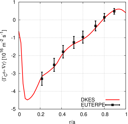
Figure 1: EUTERPE/DKES comparison for the radial particle flux density of C⁶⁺ as a function of the effective radius normalized to the minor radius $r/a$. The plasma parameters correspond to the case B.III shown in fig. 3.

Regarding the calculation of $\Phi_{1}$, instead of the less restrictive ambipolariy constraint $\sum_{\alpha}Z_{\alpha}e\left<\Gamma_{\alpha}\cdot\nabla r\right>=0$ that determines the ambipolar part of the electrostatic potential $\Phi_{0}$, the calculation of $\Phi_{1}$ requires the fulfillment of quasi-neutrality among all the species ${\alpha}$,

$$\sum_{\alpha}q_{\alpha}n_{\alpha}=0.$$ (11)

Taking the density for the species $\alpha$ up to first order as the sum of the equilibrium part $n_{\alpha 0}$ (now varying on the flux surface due to the adiabatic response) and the first order departure

$$n_{\alpha}=n_{\alpha 0}\exp(-Z_{\alpha}e\Phi_{1}/T_{\alpha})+n_{\alpha 1},$$ (12)

yields to the following relation in the approximation $Ze\Phi_{1}/T\ll 1$

$$\Phi_{1}=\frac{T_{e}}{e}\left(n_{0e}+n_{0i}\frac{T_{e}}{T_{i}}+Z^{2}n_{0Z}\frac{T_{e}}{T_{Z}}\right)^{-1}\left(n_{1i}+n_{1e}+Zn_{1Z}\right).$$ (13)

For the calculations carried out in this work the electron response has been assumed adiabatic. In addition the concentration is set sufficiently low in all cases ($Z_{\text{eff}}=1.1$) to justify the tracer impurity limit taken into account and neglect the contribution of $n_{1Z}$ to $\Phi_{1}$. The relaxation of this assumption indeed may conflict with the truncation applied to the Taylor series of the adiabatic part so to keep it linear in $\Phi_{1}$ for the impurity distribution function since, as it is shown in next section $Z_{\alpha}e\Phi_{1}/T_{\alpha}$ can become of order unity. Considering more terms in the expansion of the Boltzmann response would lead then to a non linear quasi-neutrality equation, whose complexity if left out of the scope of this paper. Thust, under the assumptions aforementioned the resulting equation for $\Phi_{1}$ reduces to,

$$\Phi_{1}=\frac{T_{e}}{e}\left(n_{0e}+n_{0i}\frac{T_{e}}{T_{i}}\right)^{-1}n_{1i},$$ (14)

and reflects that the potential required to balance the lack of charge quasi-neutrality at zeroth order is guaranteed by the first order depature from the equilibrium density of the bulk ion species, $H^{+}$ throughout all the work.

On the numerical side, the Fourier solver implemented in EUTERPE applies a low mode number filter to solve the quasi-neutrality equation that selects the modes in the intervals $[-4,4]$ in the poloidal mode number $m$, and $[0,4]$ in the toroidal one $n$. Note that $\Phi_{1}(\theta,\phi)$ is obtained at each flux surface separately. As it is different at each of them a radial dependency that is not taken into account in the Vlasov equation 10 is present. Furthermore, since $\Phi_{1}$ is obtained at every time step makes that formally the dependence of $\Phi_{1}$ is more correctly expressed as $\Phi_{1}(r,\theta,\phi,t)$. Nevertheless, on the one hand the radial dependency can be neglected since the radial electric field related to $\Phi_{1}$ is negligible respect to the ambipolar part: $\partial\Phi_{1}/\partial t\ll\text{d}\Phi_{0}/\text{d}r$. And regarding the time dependency, this is averaged out in the time interval when the stationary conditions have been reached. Then, for the remeinder of this paper we will assume the dependence of $\Phi_{1}$ as it is actually felt by the tracer impurities in our calculations of their fluxes, just a stationary potential $\Phi_{1}(\theta,\phi)$ plugged into eq. 10 to which impurities do not contribute given its low concentration. Thus the nonlinear feedback of the impurity density inhomogeneity on themselves through its impact on $\Phi_{1}$ is kept out of the scope of this work as well. An example of such map with the corresponding spectrum represented with the absolute values of the real and imaginary parts of the complex Fourier coefficients normalized to the component with maximum amplitude is shown in fig. 2. We advance that these example figure correspond to the case B.III discussed later in section 3.1.

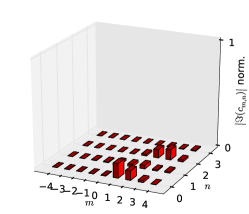
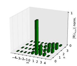
Figure 2: (Left) Stationary solution of $\Phi_{1}$ obtained with EUTERPE as a function of the poloidal and toroidal coordinates $\theta$ and $\phi$. Real and imaginary parts (left and right respectively) of the Fourier coefficients $\Phi_{1,mn}$ on the filtered modes window, and normalized to the modulus of the largest component, in this case $\cos\theta$.

3 Radial flux of C⁶⁺ including $\Phi_{1}$

In this section the numerical results are presented and discussed. Three different non-axisymmetric devices have been considered: the heliotron type Large Helical Device (LHD, Toki, Japan); the helias type Wendelstein 7-X (W7-X, Greifswald, Germany) and the heliac TJ-II (Madrid, Spain). For each of them a vacuum configuration has been used and the radial particle flux of C⁶⁺ calculated, comparing the result when $\Phi_{1}$ is neglected with the result when $\Phi_{1}$ is taken into account. The plasma parameters scanned have resulted in 6 different sets of density and temperature profiles for LHD, 4 for W7-X and 2 for TJ-II. The paramenters related to the magnetic configuration for these three devices are listed in table 1.

Magnetic configurations
Device	$B_{0,0}(r/a=0.5)$ [T]	$R$ [m]	$a$ [a]
LHD	1.54	3.6577	0.5909
Wendelstein 7-X	2.78	5.5118	0.5129
TJ-II	0.996	1.5041	0.1926

Table 1: Major and minor radii, $R$ and $a$ respectively, and amplitude of the Boozer harmonic $(m,n)=(0,0)$ of the magnetic field at the mid plasma radius, $B_{0,0}$.

3.1 LHD results

For the LHD two different density profiles have been considered. A first one corresponding to a high density scenario and a second one corresponding to a low density one. These two profiles are represented in fig. 3 (left) and labeled respectively as A (high density) and B (low density). The equilibrium density $n_{0i}$ of the bulk ions (Hydrogen nuclei) and impurities $n_{0Z}$ – in all cases fully ionized Carbon C⁶⁺ – is determined so to fulfill quasi-neutrality among these and the electrons: $\sum_{\alpha}Z_{\alpha}en_{0\alpha}=0$. The reference value considered for the effective charge is for all cases $Z_{\text{eff}}=1.1$, that allows to assume negligible the impact of the radial flux of Carbon on the ambipolar electrostatic potential $\Phi_{0}$, and of the influence of the impurity perturbed density $n_{1Z}$ on the potential $\Phi_{1}$. Three temperature profiles for C⁶⁺, set equal to the bulk ion temperature $T_{i}$, have been used, letting the electron temperature $T_{e}$ profiles fixed. These profiles, sorted by increasing ion temperature are labeled as I, II and III, and are shown in fig. 3 (center). Finally the magnetic field strength of the magnetic configuration is at the position $r/a=0.6$ illustrated in fig. 3 (right) as a function of the poloidal and toroidal angular coordinates $\theta$ and $\phi$.

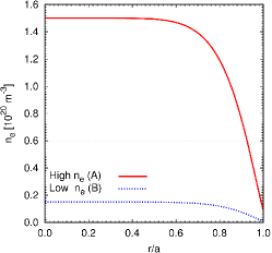
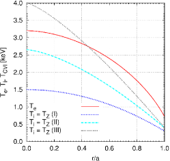
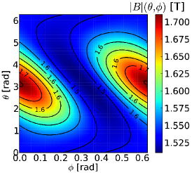
Figure 3: Set of profiles considered for the LHD cases. (Left) Electron density profiles. (Center) Electron, Hydrogen and C⁶⁺ temperature profiles. (Right) Magnetic field modulus in one LHD field period at the radial position $r/a=0.5$.

In fig. 4 for the low density set of profiles A the electrostatic potential depending on the poloidal and toroidal coordinates $\Phi_{1}(\theta,\phi)$ is represented on the top row for the three mentioned ion and C⁶⁺ temperature profiles I, II and III. Equivalently the bottom row contains for the low density set B the three maps of $\Phi_{1}$ for the same three temperature profiles. All the six maps are considered at the radial position $r/a=0.6$.
It can be observed the qualitative trend mentioned in the introduction. As the maps are viewed from left to right and top to bottom, this is with monotonically decreasing ion collisionality, the variation of the potential from peak to peak is increased in one order of magnitude, accordingly with the decrease of the collisionality (of a factor 40 approximately). This justifies to some extent the neglect of the electron contribution to $\Phi_{1}$ we are considering, since in the cases considered the electron to ion collisionality is also of the same order larger than that of the bulk ions.

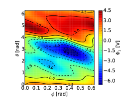
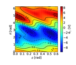
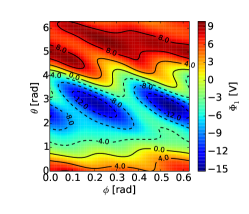
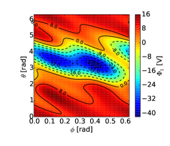
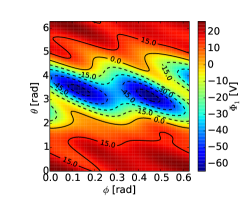
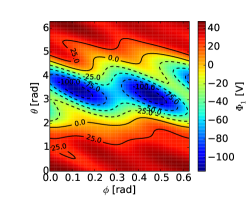
Figure 4: At the position $r/a=0.6$ for LHD: on the top row $\Phi_{1}(\theta,\phi)$ for the high density case (A) and on the bottom row for the low density case (B). The left, center and right column corresponds to the temperature profiles considered I, II and III respectively.

Regarding the central question of how strongly is the impurity transport affected by $\Phi_{1}$, the potential was calculated at the radial positions $r/a=\left\{0.2,0.4,0.6,0.8\right\}$ for each set of profiles, and the resulting maps of $\Phi_{1}$ considered as an input for the calculation of the C⁶⁺ radial particle flux $\left<\boldsymbol{\Gamma}\cdot\nabla r\right>$. The radial particle flux density of C⁶⁺ as a function of the flux surface label is shown in fig. 5 for each of the 6 profiles sets considered in this section, and normalized to the equilibrium impurity density $n_{0Z}$. The dotted line represents the case where only the ambipolar electric field is taken into account, and the solid onee corresponds to the case where both the ambipolar part of the potential $\Phi_{0}$ and $\Phi_{1}$ are both taken into account. Each of the 6 plots is accordingly displayed at the same position than the maps in fig. 4 do refered to the pair of profiles considered. This is, on the top row the high density scan A and on the bottom one the low density one B are shown; and from left to right the figures corresponds to the $T_{i}=T_{\text{\tiny{C${}^{6+}$}}}$ profile I (left), II (center) and III (right).

At a first glance, reading the plots of fig. 5 from left to right and top to bottom and looking at the maps in 4 as orientative for the order of magnitude of $\Phi_{1}$ for each case (note that the maps shown are for the position $r/a=0.6$ only), it is found that the impact that $\Phi_{1}$ produces on the ratial particle flux of Carbon is continuously increasing as $\Phi_{1}$ does. And interestingly, the modification that this represents respect to the standard neoclassical picture does not point always to the same direction. $\Phi_{1}$ both mitigates and amplifies the trend of C⁶⁺ to accumulate. On the one hand, in the high density scan (three figures on top) the impact of $\Phi_{1}$ results in a weak mitigation of the inwards flux at all radial positions considered, almost negligible in the lowest $T_{i}$ case (top, left) but appreciable in the highest $T_{i}$ one (top, right). On the other hand, the three figures at the bottom corresponding to the low density temperature scan coincide to the fact that $\Phi_{1}$ reduces the inwards Carbon flux at the internal radial positions below $r/a=0.4$ approximately and makes it stronger from there outwards, resulting in the less collisional of all the cases considered B.III (bottom, right) in the reversal of the behavior predicted by the standard neoclassical approach and a substantial reduction of the inwards flux.

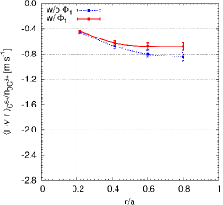
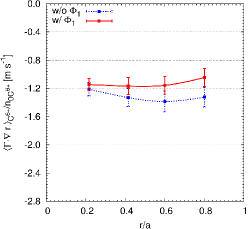
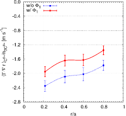
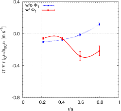
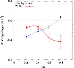
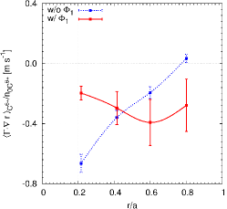
Figure 5: Radial flux density of C⁶⁺ as a function of $r/a$ including $\Phi_{1}$ (solid line) and neglecting it (dotted line). From left to right the temperature profiles I, II and III are considered and from top to bottom the high A and low B density cases.

In order to sketch qualitatively what underlies the fact that the radial flux predicted by the standard neoclassical prediction becomes stronger or weaker when $\Phi_{1}$ is taken into account, in fig. 6 the real and imaginary part of the complex Fourier coefficients of $\Phi_{1}$, or equivalently the amplitude of cosine and sine components, is presented at each position simulated in the set of figs. 5. Each of the plots in figs. 6 refers to that at the same position in figs. 5. All the cases point out to the fact that the main components are the $\cos\theta$ and $\sin\theta$, and that a correlation between the sign of the latter, plus/minus, corresponds respectively to the situation where less/ more inwards flux is driven. This is remarkably clear in the low density temperature scan. Looking at the three plots at the bottom of the figures 5 and the corresponding Fourier coefficient at the bottom row of figs. 6, the transition from a mitigated to an enhanced inwards flux accurs approximately at the radial position where the sign of the $\sin\theta$ component flips the sign.

It is important, in oder to provide an idea of the more complex coupling of $\nabla\Phi_{1}$ (in comparison with $\nabla B$) to $f_{1}$ and produce transport, the presence of sine components in the spectrum of $\Phi_{1}$. This point out to the lack of the stellarator symmetry that for instance the magnetic field modulus $B$ has. It is indeed the stellarator symmetry of $B$ what makes a necessary condition its absence in $\Phi_{1}$. Considering the radial flux density of particles expressed as

$$\left<\boldsymbol{\Gamma}\cdot\nabla r\right>=\left<\int\text{d}^{3}v\frac{\text{d}r}{\text{d}t}f_{1}\right>,$$ (15)

where $\left<...\right>$ is the flux surface average. For the bulk ion neoclassical flux it can be written as $\text{d}r/\text{d}t\approx\mathbf{v}_{\text{d}}\cdot\nabla r$. This term introduces derivatives respect to $\theta$ and $\phi$ in the integrand of 15 that makes that a stellarator symmetric magnetic field does not drive any transport unless the distribution function indeed develops sine components. This sine components are then inherited by the moments of the perturbed part of the distribution function like the perturbed density and subsequently the electrostatic potential $\Phi_{1}$. Regarding the impurity radial particle transport one needs to recover the initial hypothesis that retaining $\mathbf{v}_{E1}$ is necessary and express $\text{d}r/\text{d}t\approx\left(\mathbf{v}_{\text{d}}+\mathbf{v}_{E1}\right)\cdot\nabla r$. Then, regarding how $\Phi_{1}$ participates on the transport of impurities becomes less trivial than for the case of $B$, given that $\Phi_{1}$ Fourier spectrum has both sine and cosine parts that drives particle flux coupled to the perturbed distribution function through both its cosine and sine components respectively, and not only through the latter ones as $\mathbf{v}_{d}$ does. To this respect the question of how efficient can a specific component of $\Phi_{1}$ be in counteracting the trend of the impurities to accumulate depends on the spatial dependence of their distribution function, and brings to the same importance the the knowledge of $\Phi_{1}$ and the impurity density variation on the flux surface. An indeed, both magnitudes have recently met an increasing interest in their measurement [17, 18, 19]. is kept out of the scope of this paper will be addressed in future works.

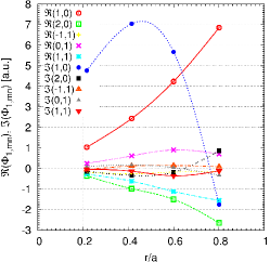
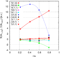
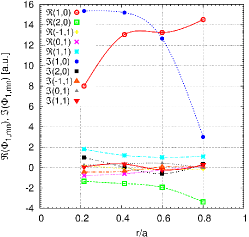
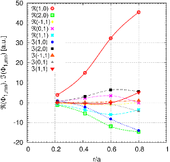
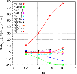
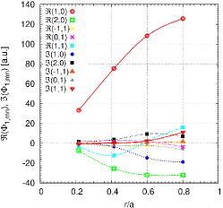
Figure 6: Amplitude of the main Fourier components as a function of the radial position for the six cases considered, displayed as in figs. 5.

3.2 Wendelstein 7-X results

The main features of the dependence of $\Phi_{1}$ with the plasma parameters, as well as the role of its Fourier spectrum on supporting or reducing the tendency of C⁶⁺ to accumulate have been discussed in sec. 3.1. In this one we show similar numerical simulations for the Wendelstein 7-X stellarator, and a set of profiles expected under operation. These are shown in fig. 7. The electron density profile is represented in fig. 7 (left), and as before $Z_{\text{eff}}=1.1$ is considered to determine $n_{0i}$ and $n_{0Z}$. The temperature, the same for all species in each of the two cases, is the parameter scanned. Four different profiles have been considered. The temperature profiles in fig. 7 (center) are labeled as I, II, III and IV increasingly with $T$.

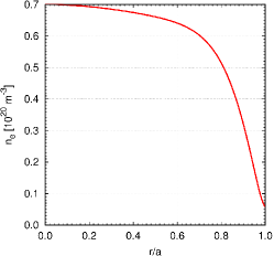
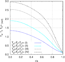
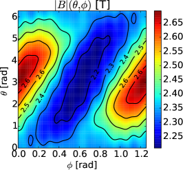
Figure 7: Set of profiles considered for W7-X. (Left) Electron density profile. (Center) Electron, bulk ion and C⁶⁺ temperature profiles, assumed the same for all the three species. (Right) Magnetic field modulus in one W7-X period at the position $r/a=0.6$.

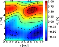
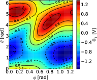
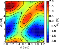
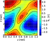
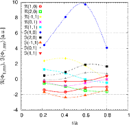
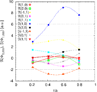
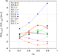
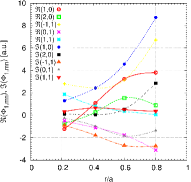
Figure 8: At the position $r/a=0.6$ for W7-X, $\Phi_{1}(\theta,\phi)$ for the temperature profiles I, II,III and IV (from left to right).

The electrostatic potential is in this case appreciably much lower than at LHD. Although the collisionality does not reach in any of the the four cases considered in this section the value of the lowest collisional low density LHD set B, the variation of the potential is noticeably much lower in W7-X for a similar collisionality.

A possible reason underlying the low electrostatic potential variation in W7-X is the physical target for the design of this device, namely, reducing the neoclassical losses and bootstrap current by approaching an omnigeneous magnetic field structure. In a perfect omnigeneous magnetic field the bounced-averaged drift orbits of the localized particles align to the flux surfaces. Although this ideal situation is not, and cannot be [20], the case, the closer the W7-X magnetic field structure is from it – compared to the other devices considered in this work – certainly leads to a smaller departure of the localized particles from the flux surfaces and results in a weaker electrostatic potential variation on them. Regarding the Fourier spectrum of $\Phi_{1}$, similar features to LHD’s at similar collisionality (cases A.I-III) are shown. A dominant $\sin\theta$ component, and a weaker $\cos\theta$ one that increases as collisionalily decreases is the footprint of the electrostatic potential in both $W7-X$ and LHD, although the rest of the modes represent a more noticeable contribution to the spectrum of $\Phi_{1}$ than in LHD, where they are all marginally zero with a some exception (e.g. the $\cos 2\theta$).

The radial profiles for the particle flux density of C⁶⁺ are represented in fig. 9 in the three W7X cases, increasing the temperature from the left to the right. Not surprisingly the difference that $\Phi_{1}$ makes respect to the standard neoclassical prediction can be well considered for the present set of parameters and impurity species negligible and aligned to the neoclassical optimization aforementioned.

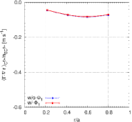
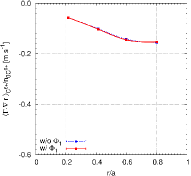
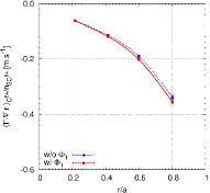
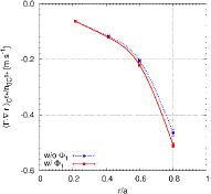
Figure 9: Radial flux density of C⁶⁺ as a function of $r/a$ including $\Phi_{1}$ (solid line) and neglecting it (dotted line). The cases I to IV are represented from left to right.

3.3 TJ-II results

Finally in the present section two cases are considered for the TJ-II stellarator. Two density profiles, shown in fig. 10(left), at a fixed temperature for the electrons and bulk and impurity ions ($H^{+}$ and C⁶⁺ as in the previous cases) represented in fig. 10(center). These profiles correspond to typical NBI-heated TJ-II plasmas. The contour plot of the magnetic field at the flux surface $r/a=0.6$ is represented in fig. 10(right).

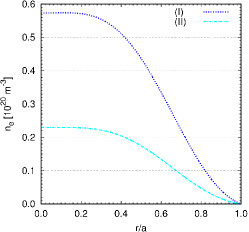
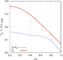
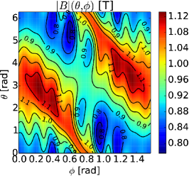
Figure 10: Set of profiles considered for TJ-II. (Left) Electron density radial profile. (Center) Electron, bulk ion and C⁶⁺ temperature profiles, assumed all equal. (Right) Magnetic field modulus in one TJ-II period at the position $r/a=0.6$.

In fig. 11 (top) the electrostatic potential $\Phi_{1}$ is represented for the two cases considered together with some Fourier harmonics (bottom). The calculation of $\Phi_{1}$ performed shows a low $\Phi_{1}$ amplitude compared to the LHD cases, and of the same order of magnitude of a few volts as in W7-X. Nevertheless, the much lower temperature (and higher collisionality) in this TJ-II sample compared to those considered for the previous two devices, leads indeed to conclude that TJ-II exhibits the strongest potential variation of the three, specially if the electrostatic energy variation related to $\Phi_{1}$ is compared to the thermal one. A discussion on this comparison for all the cases considered in the present work is given in section 4. We advance that the electrostatic potential variation for the bulk ions reaches up to a 5-8 % of the thermal energy for the low density TJ-II case and up to 10-15 % for the low density one, but despite of this the radial transport when $\Phi_{1}$ is included is not as different from the prediction without it could be expected. This can be observed in figs 12(left) and 12(right) where the comparison of radial particle flux density with and without $\Phi_{1}$ is represented for the high and low density cases respectively.

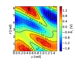
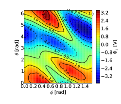
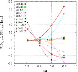
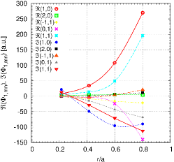
Figure 11: At the position $r/a=0.6$ for TJ-II standard configuration: $\Phi_{1}(\theta,\phi)$ for the temperature profiles I (left) and II (right).

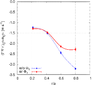
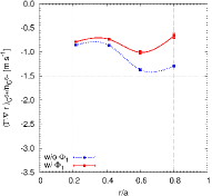
Figure 12: Radial particle flux density of C⁶⁺ as a function of $r/a$ including $\Phi_{1}$ (solid line) and neglecting it (dotted line), for the high and low density cases (left and right respectively).

A possible explanation could rest on the broad spectrum that $\Phi_{1}$ exhibits in TJ-II, and that could lead to a partial cancellation of the effect of Fourier components contributing both to enlarge and diminish the flux level. In fig. 11 (bottom) the main Fourier components are respectively represented as a function of $r/a$ for the high density case (left) and low density one (right), showing the absence of a clear dominant component. Although the $\cos\theta$ term is large along the radial coordinate in both cases, its amplitude is not much larger than other terms similarly large, as e.g the $\sin\theta$, the helical components $\cos(\theta+\phi)$, $\sin(\theta+\phi)$ or $\sin\theta$.

4 Final remark on the amplitude of $\Phi_{1}$

In fig. 13 the maximum variation of electrostatic energy for H⁺ related to the difference between the maximum and minimum value of the potential on the surface $\Delta Phi_{1}$ is represented, as a function of the normalized collision frequency normalized to the bounce frequency, $\nu^{*}=\nu_{i,\text{th}}/\omega_{b}$, with $\omega_{b}=v_{\text{th}}\iota/R$. This ratio $e\Delta\Phi_{1}/T$ is represented for all the cases considered in the work at the four radial positions considered in each case. The value $e\Delta\Phi_{1}/T$ provides an estimate of how reliable is the standard neoclassical assumption of mono-energetic trajectories for the bulk ions, and if multiplied by the corresponding charge state, for the impurity species of interest.
To this respect, having taken C⁶⁺ as the impurity for the present study, it is clear that the mono-energetic assumption breaks down in the LHD and TJ-II cases at the most external position $r/a=0.6$ and $0.8$, that correspond to the uppermost points of each curve. This is remarkably clear at the low collisional LHD set of profiles and the two cases in TJ-II. In TJ-II the potential variation is particularly large considering the much larger collisionality than in the LHD set B, as it was noted at the end of the previous section. At similar collisionality, comparing the LHD set case A.I and TJ-II low density one, LHD shows roughly an order of magnitude lower $\Phi_{1}$ than TJ-II. Note that in this normalized picture the ratios comparing the strength of $\nabla\Phi_{1}$ and $\nabla B$ as transport and trapping sources in eqs. 5 and 6 become of order unit as well.
In the figure it can be appreciated how at similar collisional regime W7-X reaches values of $e\Delta\Phi_{1}/T$ one order of magnitude lower that in the LHD high density set, and finds the usual neoclassical neglect of $\Phi_{1}$ well valid for the parameters considered.

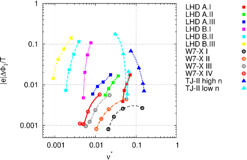
Figure 13: Normalized peak-to-peak variation of the potential $\Delta\Phi_{1}$ for all cases considered for LHD, W7-X and TJ-II as a function of the normalized thermal collision frequency of bulk the ions normalized to the bounce frequency $\omega_{b}$.

5 Summary and conclusions

The impurity transport is known to be strongly influenced by the ambipolar part of the electrostatic potential, usually considered as an approximation to the full neoclassical electrostatic potential. In the present work, we have also considered the potential variation on the flux surface $\Phi_{1}$ after solving the quasi-neutrality equation, and calculated the impact on the radial particle flux of C⁶⁺ for the devices LHD, W7-X and TJ-II, using the code EUTERPE.
The calculation have confirmed the initial assumptions on the importance of taking $\Phi_{1}$ into account for the transport of impurities, given that for these $\Phi_{1}$ can both modifying substantially the topology of the trapped/passing boundaries or driving transport through the related $E\times B$ drift in the same degree than $\nabla B$.
In most cases $\Phi_{1}$ has led to appreciable deviations from the results framed in the standard neoclassical approach, both mitigating or enhancing the trend to accumulate. This was particularly clear in the LHD low collisional cases, and in less extent in the higher collisional TJ-II ones, despite the large variation of $\Phi_{1}$ the latter device exhibit. Finally in W7-X $\Phi_{1}$ has resulted to be weak enough to be negligible for the equilibrium and parameters considered.
Although an extension of previous studies, and apart from a more exhaustive parameter and magnetic configuration scan, there are still major points to address and assumptions to relax in next works: first of all the relaxation of the tracer impurity limit, since scenarios with accumulation unavoidably can lead in long discharges to sufficiently high impurity concentration to make this approximation break down; once impurities are no longer tracers and must be included in the quasi-neutrality equation the linear adiabatic response considered, specially if they have large charge states, is no longer valid either; a detailed study of how $\Phi_{1}$ and the spacial impurity distribution function couples to each other could also help to identify what phase shift between both can bring mitigated accumulation scenarios.

6 Acknowledgements

This work was supported by EURATOM and carried out within the framework of the European Fusion Development Agreement. The views and opinions expressed herein do not necessarily reflect those of the European Commision.
The calculations were carried out using the HELIOS supercomputer system at Computational Simulation Centre of International Fusion Energy Research Centre (IFERC-CSC), Aomori, Japan, under the Broader Approach collaboration between Euratom and Japan, implemented by Fusion for Energy and JAEA.

References

References

- [1] K Ida et al., Phys. Plasmas 16 056111 (2009).
- [2] M. Yoshinuma et al., Nuclear Fusion 49 062002 (2009).
- [3] A Kallenbach et al., Plasma Phys. and Control. Fusion 55 124041 (2013).
- [4] D D.-M Ho and R M Kulsrud, Phys. Fluids 30(2) 442–461 (1987).
- [5] C D Beidler et al., Nuclear Fusion 51 076001 (2011).
- [6] H Maaberg, C D Beidler, and E E Simmet, Plasma Phys. and Control. Fusion 41 1135 (1999).
- [7] H E Mynick, Physics of Fluids 27(8) 2086 (1984).
- [8] C D Beidler and H Maberg, 15th International Stellarator Workshop, Madrid (2005).
- [9] J M García-Regaña et al., Plasma Phys. and Control. Fusion 55 074008 (2013).
- [10] V Kornilov et al., Nuclear Fusion 45(4) 238 (2005).
- [11] T Takizuka, Journal of Computational Physics 25(3) 205–219 (1977).
- [12] K Kauffmann et al., J. Phys.: Conf. Ser. 260(1) 012014 (2010).
- [13] Y. Turkin et al. Physics of Plasmas 18 022505 (2011).
- [14] S P Hirshman et al., Physics of Fluids 29 2951 (1986).
- [15] W. I. van Rij and S. P. Hirshman, Physics of Fluids B 1 563 (1989).
- [16] C D Beidler and H Maberg, Plasma Phys. and Control. Fusion 43 1131–1148 (2001).
- [17] E Viezzer et al. Plasma Phys. and Control. Fusion 55 124037 (2013).
- [18] J Arévalo et al., Nuclear Fusion 54 013008 (2014).
- [19] M A Pedrosa et al., submitted to Nuclear Fusion (2014), preprint: http://arxiv.org/abs/1404.0932.
- [20] D A Garren and A H Boozer, Physics of Fluids B 3 2822 (1991).