Characterization of random stress fields obtained from polycrystalline aggregate calculations using multi-scale stochastic finite elements

Abstract

The spatial variability of stress fields resulting from polycrystalline aggregate calculations involving random grain geometry and crystal orientations is investigated. A periodogram-based method is proposed to identify the properties of homogeneous Gaussian random fields (power spectral density and related covariance structure). Based on a set of finite element polycrystalline aggregate calculations the properties of the maximal principal stress field are identified. Two cases are considered, using either a fixed or random grain geometry. The stability of the method w.r.t the number of samples and the load level (up to 3.5 % macroscopic deformation) is investigated.

Keywords: Polycrystalline aggregates – Crystal plasticity – Random fields – Spatial variability – Correlation structure

1 Introduction

In pressurized water reactors of nuclear plants, the pressure vessel constitutes one element of the second safety barrier between the radioactive fuel rods and the external environment. It is made of 16MND5 (A508) steel which is forged and welded. In case of operating accidents such as LOCA (loss of coolant accident), the pressure vessel is subjected to a pressurized thermal shock due to fast injection of cold water into the primary circuit. If some defects (e.g cracks) were present in the vessel wall this may lead to crack initiation and propagation and the brittle fracture of the vessel. The detailed study of the embrittlement of 16MND5 steel under irradiation is thus a great concern for electrical companies such as EDF.

The brittle fracture behavior of the 16MND5 steel has been thoroughly studied in the last decade using the local approach of fracture theory (Tanguy, 2001) and the so-called Beremin model (Beremin, 1983), which assumes that cleavage is controlled by the propagation of the weakest link between a population of pre-existing micro-defects in the material. This approach has been recently coupled with polycrystalline aggregates simulations (Mathieu et al, 2006), (Mathieu et al, 2010).

The main idea is to model a material representative volume element (RVE) as a polycrystalline synthetic aggregate and compute the stress field under given load conditions. As a post-processing a statistical distribution of defects (carbides) is sampled over the volume. In each Gauss point of the finite element mesh the cleavage criterion is attained somewhere along the load path if a) the equivalent plastic strain has attained some threshold (cleavage initiation) and b) a Griffith-like criterion applied to the size of the carbide in this Gauss point is reached (cleavage propagation). Within the weakest link theory the failure of a single critical carbide induces the failure of the RVE.

From a single RVE simulation (i.e. a single stress field) various distributions of carbides are drawn, each realization leading to a maximal principal stress associated to failure. Then the distribution of these quantities is fitted using a Weibull law (Mathieu et al, 2010). In such an approach, the current practice of computational micromechanics assumes that the RVE is large enough to represent the behavior of the material so that a single polycrystalline analysis is carried out (the large CPU required by polycrystalline simulations also favours the use of a single simulation). However it is believed that numerous parameters such as grain geometry and orientation may influence the stress field and thus the final result.

The connection between micromechanics and stochastic methods has been given much attention in the past few years, as shown in Graham-Brady et al (2006); Stefanou (2009); Xu and Chen (2009). Many papers are devoted to developing probabilistic models for reproducing a random microstructure, e.g. Graham and Baxter (2001); Liu et al (2007); Chung et al (2005); Chakraborty and Rahman (2008). The specific representation of polycrystalline microstructures has been addressed in Arwade and Grigoriu (2004); Grigoriu (2010); Li et al (2010); Kouchmeshky and Zabaras (2010) among others. The propagation of the uncertainty on the microstructure through a micromechanical model in order to study the variability of the resulting strain and stresses has not been addressed much though (see e.g. Kouchmeshky and Zabaras (2009)).

In this paper it is proposed to identify the properties of a stress random field resulting from the progressive loading of a polycrystalline aggregate. More precisely, assuming that the stress random field is Gaussian, a procedure called periodogram method is devised, which allows one to identify the correlation structure of the resulting stress field.

The paper is organized as follows: in Section 2 basics of Gaussian random fields are recalled and the periodogram method is presented (Dang et al, 2011b). The polycrystalline aggregate computational model is detailed in Section 3. The methodology for identifying the correlation structure of the resulting stress field is presented in Section 4. Two application cases are then investigated, namely an aggregate with fixed grain boundaries and random crystallographic orientations (Section 5) and an aggregate with both random geometry and orientations (Section 6). The variance of the resulting stress field as well as the spatial covariance function and its correlation lengths is investigated in details. The properties of the identified random fields will be used in a forthcoming study in the context of the local approach to fracture, as explained above.

2 Inference of the properties of a Gaussian random field

In this section an identification method called periodogram is presented, which uses an estimator of the Power Spectral Density (PSD) in order to identify the correlation structure of a Gaussian homogeneous random field. Based on original developments by Stoica and Moses (1997) and Li (2005) for unidimensional fields, it has been extended to two-dimensional cases by Dang et al (2011b). As it relies upon the use of the Fast Fourier Transform (FFT) its computational efficiency is remarkable.

2.1 Definitions

A Gaussian random field $Z(\boldsymbol{x},\omega)$ is completely defined by its mean value $\mu(\boldsymbol{x})$, its standard deviation $\sigma(x)$ and its auto-covariance function $C(\boldsymbol{x},\boldsymbol{x}^{\prime})$. It is said homogeneous if the mean value $\mu(\boldsymbol{x})$ and the standard deviation $\sigma(\boldsymbol{x})$ are constant in the domain of definition of $\boldsymbol{x}$ and the auto-covariance function $C(\boldsymbol{x},\boldsymbol{x}^{\prime})$ only depends on the shift $\boldsymbol{h}=\boldsymbol{x}-\boldsymbol{x}^{\prime}$. Let us introduce the $n-$th statistical moment $m^{n}_{Z}$ and the spatial average $m^{n}_{\boldsymbol{V}}$:

$$m^{n}_{Z} ={\mathbb{E}}\left[Z^{n}(\boldsymbol{x}_{0},\omega)\right]=\int\limits_{-\infty}^{\infty}z^{n}(\boldsymbol{x}_{0},\omega)f_{Z}(z,\boldsymbol{x}_{0})dz$$ (1)

$$m^{n}_{\boldsymbol{V}} =\lim\limits_{\boldsymbol{V}\rightarrow\infty}\frac{1}{\boldsymbol{V}}\int\limits_{V}z^{n}(\boldsymbol{x},\omega_{0})d\boldsymbol{x}$$ (2)

The field is said ergodic if its ensemble statistics is equal to the spatial average, i.e. $m^{n}_{Z}=m^{n}_{\boldsymbol{V}}$ (Cramer and Leadbetter, 1967). Several popular covariance models for two-dimensional homogeneous random fields are presented in Table 1. In this table, $\sigma$ is the constant standard deviation of the field, $h_{1},h_{2}$ are the components of the shift $\boldsymbol{h}$ in the two directions, $l_{1},l_{2}$ are the correlation lengths in the two directions. Gaussian and exponential models are plotted in Figure 1 for the sake of illustration. Note that we call correlation length the parameters that appear in the definition of the covariance functions. This is not to be confused with the scale of fluctuation (Vanmarcke, 1983), which combine both the shape of the covariance function and the lengths $l_{1},l_{2}$. In one dimension, denoting by $\rho(x;\,l)$ the autocorrelation function, the scale of fluctuation may be defined by:

$$2\,l_{c}=\int_{-\infty}^{\infty}\rho(x;\,l)\,dx$$

which reduces to $l_{c}=l$ for the exponential correlation function and $l_{c}=\sqrt{\pi}/2\approx 0.886\,l$ for the Gaussian case. Similar expression are available in two and three dimensions, see e.g. Xu and Chen (2009).

Table 1: Covariance functions and associated power spectral densities for homogeneous twodimensional random fields

Model	Covariance function	Power spectral density
Exponential	$\sigma^{2}\mbox{exp}\left[-(\frac{|h_{1}|}{l_{1}}+\frac{|h_{2}|}{l_{2}})\right]$	$\sigma^{2}\;\frac{2l_{1}}{1+4\pi^{2}l_{1}^{2}f_{1}^{2}}\;\frac{2l_{2}}{1+4\pi^{2}l_{2}^{2}f_{2}^{2}}$
Gaussian	$\sigma^{2}\mbox{exp}\left[-(\frac{h_{1}^{2}}{l_{1}^{2}}+\frac{h_{2}^{2}}{l_{1}^{2}})\right]$	$\sigma^{2}\;\pi l_{1}\mbox{exp}\left(\pi^{2}l_{1}^{2}f_{1}^{2}\right)\;\pi l_{2}\mbox{exp}\left(\pi^{2}l_{2}^{2}f_{2}^{2}\right)$
Wave	$\sigma^{2}\mbox{sinc}(\frac{|h_{1}|}{l_{1}})$sinc$(\frac{|h_{2}|}{l_{2}})$	$\sigma^{2}\;\pi l_{1}\mbox{rect}_{1}(\pi l_{1}f_{1})\;\pi l_{2}\mbox{rect}_{1}(\pi l_{2}f_{2})$
Triangle	$\sigma^{2}\mbox{tri}(\frac{|h_{1}|}{l_{1}})$tri$(\frac{|h_{2}|}{l_{2}})$	$\sigma^{2}\;l_{1}\mbox{sinc}^{2}(\pi f_{1}l_{1})\;l_{2}\mbox{sinc}^{2}(\pi f_{2}l_{2})$

$\text{sinc}(x)=\sin x/x$
$\mbox{tri(x)}=1-|x|$ if $|x|\leq 1$ and 0 otherwise
$\mbox{rect}_{\tau}(f)=1$ if $|f|\leq\frac{\tau}{2}$ and 0 otherwise

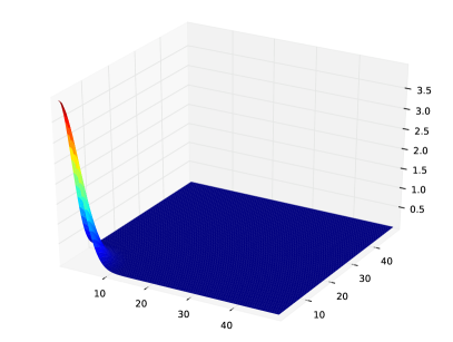
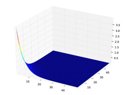
Figure 1: Gaussian covariance model (left) and Exponential covariance model (right) : $\sigma=2$, $l_{1}=l_{2}=5$

The power spectral density (PSD) of the random field is the Fourier transform of its covariance function as a result of the Wiener-Khintchine relationship (Preumont, 1990). The following relationships hold:

$$S(f_{1},f_{2})= \int\limits_{-\infty}^{\infty}\int\limits_{-\infty}^{\infty}C(h_{1},h_{2})e^{-i2\pi f_{1}h_{1}}e^{-i2\pi f_{2}h_{2}}dh_{1}dh_{2}$$ (3)

$$C(h_{1},h_{2})= \int\limits_{-\infty}^{\infty}\int\limits_{-\infty}^{\infty}S(f_{1},f_{2})e^{i2\pi f_{1}h_{1}}e^{i2\pi f_{2}h_{2}}df_{1}df_{2}$$ (4)

The PSD of the Gaussian and exponential covariance models are presented in Table 1.

2.2 Identification of a PSD

2.2.1 Empirical periodogram

One considers an ergodic homogeneous random field $Z(x_{1},x_{2})$, $(x_{1},x_{2})\in{\mathcal{D}}_{1}\times{\mathcal{D}}_{2}\subset{\mathbb{R}}^{2}$ for which a single realization $z(x_{1},x_{2})$ is available. If the random field was defined over an infinite domain, the classical estimation of the covariance function would be:

$$\hat{C}(h_{1},h_{2})=\frac{1}{4MN}\sum\limits_{n=-N}^{N-1}\sum\limits_{m=-M}^{M-1}Z(x_{1n}+h_{1},x_{2m}+h_{2})Z(x_{1n},x_{2m})$$ (5)

By definition, the Fourier transform of the covariance estimation is an estimation of the PSD.

$$\hat{S}(f_{1},f_{2})=\frac{1}{4MN}\tilde{Z}(f_{1},f_{2})\tilde{Z}^{*}(f_{1},f_{2})=\frac{1}{4MN}|\tilde{Z}(f_{1},f_{2})|^{2}$$ (6)

where $|.|$ denotes the modulus operator.

In practice, the problem is to estimate the periodogram from a limited amount of data gathered on $N\times M$ grid $\{z(x_{1i},x_{2j}),\,i=1,\,\dots\,,N;j=1,\,\dots\,,M\}$. Due to symmetry, the covariance estimation in Eq.(5) is recast as follows:

$$\hat{C}(h_{1k},h_{2l})=\frac{1}{NM}\sum\limits_{n=1}^{N-k}\sum\limits_{m=1}^{M-l}Z(x_{1n}+h_{1k},x_{2m}+h_{2l})\,Z(x_{1n},x_{2m})$$ (7)

By taking the expectation of the above equation one gets:

$$\begin{split}\mathbb{E}\left[\hat{C}(h_{1k},h_{2l})\right]&=\frac{N-k}{N}\frac{M-l}{M}\mathbb{E}\left[Z(x_{1n}+h_{1k},x_{2m}+h_{2l})Z(x_{1n},x_{2m})\right]\\ &=\frac{N-k}{N}\frac{M-l}{M}C(h_{1},h_{2})\end{split}$$ (8)

The latter equation exhibits some bias term between the expectation of the estimator and the covariance function $C(h_{1},h_{2})$. Using the symmetry of the covariance function, one can write:

$$\mathbb{E}\left[\hat{C}(h_{1k},h_{2l})\right]=w_{B}(k,l)C(h_{1},h_{2})$$ (9)

where $w_{B}(k,l)$ is the triangle window, also known as the Bartlett window (Figure 2):

$$w_{B}(k,l)=\left\{\begin{array}[]{l l}\frac{N-|k|}{N}\frac{M-|l|}{M}&\mbox{if $|k|\leq N$; $|l|\leq M$}\\ 0&\mbox{otherwise}\\ \end{array}\right.$$ (10)

Consequently the expectation of the periodogram estimation becomes:

$$\begin{split}\mathbb{E}\left[\hat{S}(f_{1k},f_{2l})\right]&=\mathcal{F}\left\{\mathbb{E}\left[\hat{C}(h_{1k},h_{2l})\right]\right\}=\mathcal{F}\{w_{B}(k,l)C(h_{1},h_{2})\}\\ &=W_{B}(f_{1},f_{2})*S(f_{1},f_{2})\end{split}$$ (11)

where $\mathcal{F}$ and $W_{B}(f_{1},f_{2})$ respectively denote the 2D Fourier transform operator and the Fourier transform of the Bartlett window and $*$ denotes the convolution product. This window tends to a Dirac pulse when $N,M$ tend to infinity and $w_{B}$ tends to a unit constant. Thus the periodogram estimation is asymptotically unbiased. However it is not consistent since its variance does not tend to zero (Preumont, 1990). Furthermore using this window leads to a convolution product which introduces additional computational burden. Hence in practice, the modified periodogram presented in the next section is used to estimate the PSD of the random field.

2.2.2 Modified periodogram

The modified periodogram is built up in order to avoid the convolution product with the transformed window $W_{B}(f_{1},f_{2})$ in Eq.(11). In this approach, the data is multiplied directly with the window $w(x,y)$ before the Fourier transform is carried out. It aims at filtering the data to limit the influence of long distance terms and to focus on the information given by the short distance terms. This leads to the following estimate:

$$\hat{S}(f_{1},f_{2})=\frac{1}{NMU}|\mathcal{F}\left\{z(x_{1},x_{2}).w(x_{1},x_{2})\right\}|^{2}$$ (12)

where $U$ is the energy of the window calculated by:

$$U=\frac{1}{D_{1}D_{2}}\sum\limits_{i=1}^{N}\sum\limits_{j=1}^{M}w^{2}(x_{1i},x_{2j})$$ (13)

and $D_{1},D_{2}$ denote the size of the two-dimensional domain ${\mathcal{D}}_{1}\times{\mathcal{D}}_{2}$. Various window functions are proposed in Preumont (1990), see Table 2. In this paper we will use mainly the Blackman window (Figure 2).

Table 2: Window functions used in the modified periodogram approach

Model	Window equation
Bartlett	$\left\{\begin{array}[]{l l}\frac{N-|k|}{N}\frac{M-|l|}{M}&\mbox{if $|k|\leq N$; $|l|\leq M$}\\ 0&\mbox{otherwise}\\ \end{array}\right.$
Hann	$\left\{\begin{array}[]{l l}\left[0.5+0.5\mbox{cos}(\frac{\pi k}{N})\right]\left[0.5+0.5\mbox{cos}(\frac{\pi l}{M})\right]&\mbox{if $|k|\leq N$; $|l|\leq M$}\\ 0&\mbox{otherwise}\\ \end{array}\right.$
Hamming	$\left\{\begin{array}[]{l l}\left[0.54+0.46\mbox{cos}(\frac{\pi k}{N})\right]\left[0.54+0.46\mbox{cos}(\frac{\pi l}{M})\right]&\mbox{if $|k|\leq N$; $|l|\leq M$}\\ 0&\mbox{otherwise}\\ \end{array}\right.$
Blackman	$\left\{\begin{array}[]{l l}\left[0.42+0.5\mbox{cos}(\frac{\pi k}{N})+0.08\mbox{cos}(\frac{2\pi k}{N})\right]\left[0.42+0.5\mbox{cos}(\frac{\pi l}{M})+0.08\mbox{cos}(\frac{2\pi l}{M})\right]&\mbox{if $|k|\leq N$; $|l|\leq M$}\\ 0&\mbox{otherwise}\\ \end{array}\right.$

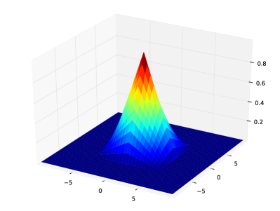
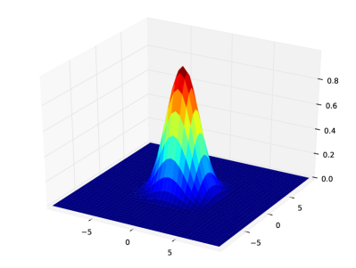
Figure 2: (a) Bartlett window ; (b) Blackman window

2.2.3 Average modified periodogram

As shown in Section 2.2.1, the estimation of the periodogram is asymptotically unbiased, however not consistent since its variance does not tend to zero when $N,M$ tend to infinity. The averaging of the modified periodogram will solve this problem. Assume that $L$ realizations of the random field are available. For each realization $z^{l}(x_{1},x_{2})$, one calculates the periodogram as in Eq.(12):

$$\hat{S}^{l}(f_{1},f_{2})=\frac{1}{NMU}|\mathcal{F}\left\{z^{l}(x_{1},x_{2}).w(x_{1},x_{2})\right\}|^{2}$$ (14)

with $1\leq l\leq L$. Then one calculates the average periodogram by:

$$\overline{S}(f_{1},f_{2})=\frac{1}{L}\sum\limits_{l=1}^{L}\hat{S}^{l}(f_{1},f_{2})$$ (15)

Therefore the variance of the average periodogram is:

$${\rm Var}\left[\overline{S}(f_{1},f_{2})\right]=\frac{1}{L}{\rm Var}\left[\hat{S}(f_{1},f_{2})\right]$$ (16)

It is then obvious that this variance tends to zero when $L$ tends to infinity, making the “average modified periodogram” approach more robust.

2.2.4 Final algorithm for PSD estimation

As a summary, the algorithm to estimate the PSD of a random field from $L$ realizations may be decomposed into the four following steps:

1. multiplication of each realization by a selected window, e.g. the Blackman window (see Table 2);

2. computation of 2D Fourier transform of the product of the current realization by the filtering window;

3. computation of the modulus of the result to obtain the PSD estimation of each realization;

4. averaging of the $L$ PSD estimations.

Once the empirical periodogram has been computed, a theoretical periodogram is selected (e.g. Gaussian, exponential, etc., see Table 1) and fitted using a least-square procedure (Marquardt, 1963). In case of multiple potential forms for the theoretical periodogram the best fitting is selected according to the smallest residual.

3 Modeling polycrystalline aggregates

In this section the computational mechanical model used in this study is presented. It simulates a tensile test on a bidimensional polycrystalline aggregate under plane strain conditions. The various ingredients are discussed, namely:

• the microstructure of the material and its synthetic representation;

• the material constitutive law;

• the boundary conditions applied onto the aggregate;

• the mesh used in the finite element simulation.

3.1 Material characterization

The material is a 16MND5 ferritic steel with a granular microstructure. The ferrite has a body centered cubic (BCC) structure. Three families of slip system should be taken into account, namely $\{110\}\langle 111\rangle$, $\{112\}\langle 111\rangle$, $\{123\}\langle 111\rangle$. However, following Franciosi (1985) it is assumed that the glides on the plane 123 are a succession of micro-glides on the planes 110, 112. This leads to consider only the two first families, which yields 24 slip systems by symmetry.

3.2 Crystal plasticity

The model for crystal plasticity chosen in this work has been originally formulated in Meric and Cailletaud (1991) within the small strain framework. The total strain rate $\dot{\varepsilon}_{ij}$ is classically decomposed as the sum of the elastic strain rate $\dot{\varepsilon}^{e}_{ij}$ and plastic strain rate $\dot{\varepsilon}^{p}_{ij}$.

$$\dot{\varepsilon}_{ij}=\dot{\varepsilon}^{e}_{ij}+\dot{\varepsilon}^{p}_{ij}$$ (17)

The elastic part follows the Hooke’s law and the plastic part is calculated from the shear strain rates of the $24$ active slip systems.

$$\dot{\varepsilon}^{p}_{ij}=\sum\limits_{g=1}^{24}\dot{\gamma}^{g}R^{g}_{ij}$$ (18)

where $\dot{\gamma}^{g}$ is the shear strain rate of the slip system $g$ and $R^{g}_{ij}$ is the Schmid factor which presents the geometrical projection tensor. The latter is calculated from the normal vector to the gliding plane n and the direction of gliding m.

$$R^{g}_{ij}=\frac{1}{2}(m_{i}n_{j}+m_{j}n_{i})$$ (19)

The Resolved Shear Stress (RSS) $\tau^{g}$ of the slip system $g$ is the projection of the stress tensor via the Schmid factor.

$$\tau^{g}=R^{g}_{ij}\sigma_{ij}$$ (20)

The shear strain rates $\dot{\gamma}^{g}$ of each slip system $g$ are the internal variable that describes plasticity. The evolution of these variables depends on the difference between the RSS $\tau^{g}$ and the actual critical RSS $\tau^{g}_{c}$ in an elastoviscoplastic setting:

$$\dot{\gamma}^{g}=\left(\frac{\tau^{g}-\tau^{g}_{c}}{K}\right)^{n}\mbox{sign}(\tau^{g})$$ (21)

where $K$ and $n$ are material constants, and $\mbox{sign}(a)=a/|a|$ if $a\neq 0$ and 0 otherwise. Note that this formula corresponds to an elastoviscoplastic constitutive law but the viscous effect will be negligible if sufficiently large values of $K$ and $n$ are selected. Its power form allows one to automatically detect the active slip systems. All the systems are considered active but the slip rate is significant only if the RSS $\tau^{g}$ is much higher than the critical RSS $\tau^{g}_{c}$. This procedure allows one to numerically smooth the elastoplastic constitutive law.

The critical RSS $\tau^{g}_{c}$ evolves according to the following isotropic hardening law:

$$\tau^{g}_{c}=\tau^{g}_{c0}+Q^{g}\sum\limits_{s=1}^{24}h^{gs}(1-e^{-b^{g}\gamma^{s}_{cum}})$$ (22)

where $\gamma^{s}_{cum}=\int\limits_{t_{0}}^{t}|\dot{\gamma^{s}}|dt$. The exponential term presents the hardening saturation in the material when the accumulated slip is high. $\tau^{g}_{c0}$ is the initial critical RSS on the considered system $g$. $Q^{g}$ and $b^{g}$ are parameters which depend on the material. $h^{gs}$ is the hardening matrix of size $24\times 24$ whose component $h^{gs}$ presents the hardening effect of the system $g$ on the system $s$. In the present work, one considers only two families of slip systems named ${110}\langle 111\rangle$, ${112}\langle 111\rangle$. Thus the hardening matrix $h^{gs}$ is completely defined by four coefficients $h_{1},h_{2},h_{3},h_{4}$ only. The values of these coefficients and this matrix are presented in Mathieu (2006). All the parameters describing crystal plasticity for 16MND5 steel are gathered in Table 3.

Table 3: Parameters of the crystal plasticity constitutive law for the 16MND5 steel (Mathieu, 2006)

Isotropic elasticity		Viscoplasticity		Isotropic hardening
$E$	$\nu$	$K$	$n$	$\tau_{c_{0}}$	$Q$	$b$	$h_{1}$	$h_{2}$	$h_{3}$	$h_{4}$
$(MPa)$		$(MPa.s^{1/n})$		$(MPa)$	$(MPa)$
$210,000$	$0.3$	$15$	$12$	$175$	$20$	$30$	$1$	$1$	$1$	$1$

3.3 Microstructure and boundary conditions

The construction of the aggregate is based on the Voronoi polyhedra model (Gilbert, 1962), generated in this work with the Quickhull algorithm (Barber et al, 1996). The geometry of the resulting synthetic aggregate, which is a simplified representation of the real microstructure of the 16MND5 steel, is shown in Figure 3. It corresponds to a square of size 1,000 (this is a relative length which shall be scaled with a real length depending on the grain size). Grain boundaries are considered as perfect interfaces. Note that more detailed models of grains have been proposed recently using so-called Laguerre tessellations (Lautensack and Zuyev, 2008) in order to better fit the observed distributions of grain size, see e.g. Zhang et al. (2011); Leonardia et al. (2012).

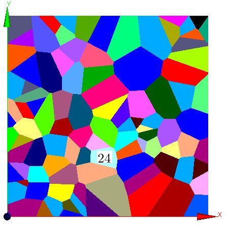
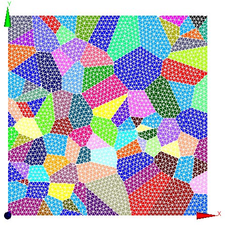
Figure 3: (a) Two-dimensional polycrystalline aggregate modelling a volume of 16MND5 steel (100 grains) (b) Mesh of the specimen (11,295 nodes)

The same crystallographic orientation, defined by the three Euler angles $\varphi_{1}$, $\phi$, $\varphi_{2}$, is randomly assigned to all integration points inside each individual grain using a uniform distribution. In Figure 3-a, the color of each grain corresponds to a given crystallographic orientation. The mesh is generated by the $BLSURF$ algorithm (Laug and Borouchaki, 1999) of the Salome software (http://www.salome-platform.org). The mesh of the generated specimen is presented in Figure 3-b. The finite elements are quadratic 6-node triangles with $3$ integration points.

The boundary conditions applied onto the aggregate are sketched in Figure 4. The lower surface is blocked along the $Y$ direction. The displacements $DX=DY=0$ are blocked at the origin of the coordinate system (lower left corner). On the upper surface, an homogeneous displacement is applied by steps in the $Y$ direction up to a macroscopic strain equal to $3.5\%$. The computation is carried out using the open source finite element software Code_Aster (http://www.code-aster.org).

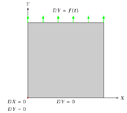
Figure 4: Boundary conditions used for simulating the tensile test

The computational cost for such a non linear analysis is high. The number of degrees of freedom of the finite element model is $33,885$. A parallel computing method based on sub-domain decomposition is used. One simulation of a full tensile test up to 3.5% strain requires about $2$ hours computation time when distributed over $4$ processors.

3.4 Results

In this section, we present the result of the simulation of a tensile test on the 2D aggregate at different scales. We define the mean stress and strain tensor calculated in a volume $V$ by:

$$\boldsymbol{\rm\Sigma}=\frac{1}{V}\int\limits_{V}\boldsymbol{\rm\sigma}dV$$ (23)

$$\boldsymbol{\rm E}=\frac{1}{V}\int\limits_{V}\boldsymbol{\rm\varepsilon}dV$$ (24)

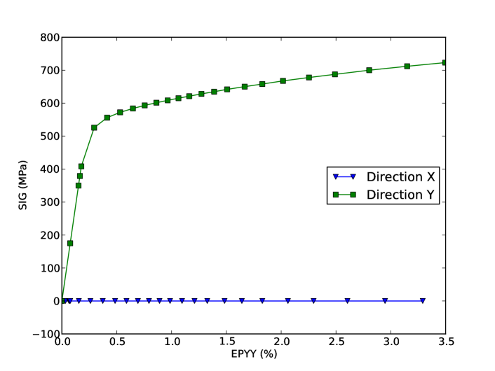
Figure 5: Macroscopic strain-stress relationship in the $X$ and $Y$ directions

Figure 5 shows the macroscopic strain/stress curve. It is observed that $\Sigma_{XX}=0$ as expected whereas the uniaxial behaviour shows a global elastoplastic behaviour.

At the mesoscopic scale one can observe the mean strain-stress relationship in each grain as shown in Figure 6. Because of the different crystallographic orientations in each grain, the mean elastoplastic behaviour is different from grain to grain. Furthermore, whereas the mean stress $\Sigma_{XX}$ calculated in all the specimen is zero, the mean values calculated in each single grain are scattered around zero. This observation shows the first scale of heterogeneity of the material.

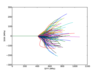
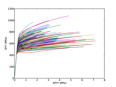
Figure 6: Mesoscopic behavior in each grain in the $X$ (left) and $Y$ (right) directions

The microscopic behaviour of a single grain (Grain #24, see tag in Figure 3) is finally studied. The mean behavior and the strain-stress relationship at each node of this grain are plotted in Figure 7 for four levels of macroscopic strain, namely $E_{YY}=0.15\%,0.65\%,1.5\%,3.5\%$.

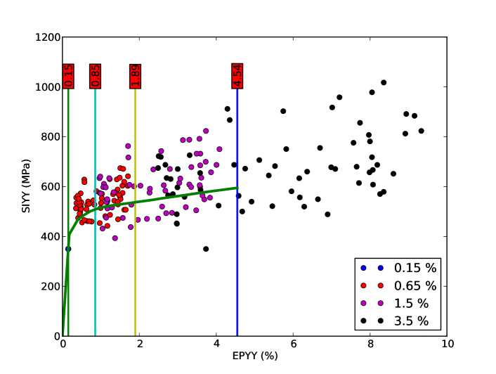
Figure 7: Microscopic strain-stress relationship for various nodes within Grain #24 and mean tensile curve

In this figure the blue point represents the stress field within the grain for a macroscopic strain level $E_{YY}=0.15\%$. This single point shows that the stress field is homogeneous within the grain in the elastic domain. The red points represent the strees values $\sigma_{YY}$ in each node of the grain at $E_{YY}=0.65\%$ macroscopic strain. One observes that the mean strain calculated for this single grain is $0.85\%$ and the maximal strain value $\varepsilon_{YY}$ in a specific node may attain about $2\%$. Similar effects are observed at other levels of macroscopic strain, which show the heterogeneity of the strain and stress fields at the microscopic scale. It is observed that the scattering around the mean curve increases with the macroscopic strain. Indeed, for the final loading step corresponding to $E_{YY}=3.5\%$ the mean strain in the grain is about 4.54%, while the local strain varies form 2.4 to 9%.

4 Identification of the maximal principal stress field

In this section the method developed in Section 2 is applied to the identification of the properties of the random stress field in polycristalline aggregate calculations. More specifically the maximal principal stress field $\sigma_{I}$ that is computed from repeated polycrystalline simulations is considered. Throughout the paper this stress field is considered Gaussian. This is a strong assumption which shall be considered as a first approximation. Indeed the maximal principal stress is positive in nature under the uniaxial loading that is considered and a Gaussian assumption cannot totally fit this feature. Yet it is believed that the results obtained in terms of the description of the spatial variability (covariance functions), which is the main outcome of the paper, will not be strongly influenced by this assumption. Note that methods for identifying the properties of non Gaussian random fields have been recently developed, see e.g. Perrin et al. (2014).

4.1 Finite element calculations and projection

The maximal principal stress field is assumed to be Gaussian and homogeneous (the latter assumption will be empirically checked as shown in the sequel). The periodogram method is applied using $K=35$ realizations of stress fields, i.e. 35 full elastoplastic analysis of aggregates up to a macroscopic strain of 3.5 %. The identification is carried out successively at various levels of the macroscopic strain. Two cases are considered:

• Case #1: the grains geometry is the same for all the finite element calculations. Only the crystallographic orientations are varying from one calculation to the other.

• Case #2: both the grains geometry and the crystallographic orientations vary.

The input data of the identification problem is the maximal principal stress field $\sigma_{I}$ obtained from the finite element calculations. As the periodogram method is based on a regular sampling of the random field under consideration, the brute result (i.e. the maximal principal stress at the nodes of the mesh) has to be projected onto a regular grid. This operation is carried out using internal routines of Code_Aster. Note that a slice of width $100$ (i.e. $10\%$ of total size) is discarded along the edges of the aggregate in order to avoid the effect of boundary conditions on the computed stress field, as suggested in Mathieu (2006). A typical maximal principal stress field is shown in Figure 8.

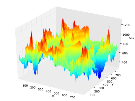
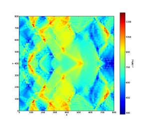
Figure 8: A realization of the maximal principal stress field $\sigma_{I}$

4.2 Check of the homogeneity of the field

As it was described in Section 2 the periodogram method assumes that the random field under consideration is homogeneous. From the available realizations $SIG_{i}(x,y),i=1,\,\dots\,,35$ one first checks empirically this assumption using the following approach:

• The ensemble mean and variance of the field is computed point-by-point throughout the grid for an increasing number of realizations $K=2,\,\dots\,,35$:

  $$\mu_{K}(x,y) = \frac{1}{K}\sum\limits_{i=1}^{K}SIG_{i}(x,y)$$ (25)

  $$\sigma^{2}_{K}(x,y) = \frac{1}{K-1}\sum\limits_{i=1}^{K}\left(SIG_{i}(x,y)-\mu(x,y)\right)^{2}$$ (26)

  If the field is homogeneous these quantities should tend to constant values that are independent from the position $(x,y)$ when $K$ tends to infinity.

• In order to measure the magnitude of the spatial fluctuation of the latter, the spatial average and spatial variance of a realization of a field $Z(x,y)$ sampled onto a $N\times M$ grid is defined by:

  $$\bar{\mu}_{Z} = \frac{1}{NM}\sum\limits_{i=1}^{N}\sum\limits_{j=1}^{M}Z(x_{i},y_{j})$$ (27)

  $$\bar{\sigma}^{2}_{Z} = \frac{1}{NM}\sum\limits_{i=1}^{N}\sum\limits_{j=1}^{M}\left(Z(x_{i},y_{j})-\bar{\mu}_{Z}\right)^{2}$$ (28)

  whereas the associated “spatial” coefficient of variation is defined by:

  $$CV_{Z}=\frac{\bar{\sigma}_{Z}}{\bar{\mu}_{Z}}$$ (29)

• The spatial coefficient of variation of the ensemble mean and variance (Eqs.(25)-(26)) are computed and plotted as a function of $K$. If the underlying random field is homogeneous it is expected that the curves of $CV_{\mu_{K}}$ and $CV_{\sigma_{K}^{2}}$ converge to zero.

4.3 Choice of theoretical periodograms and fitting

From a visual inspection of the obtained empirical periodograms it appears that a Gaussian or an exponential model of periodogram such as those presented in Table 1 may be consistent with the data. However it appeared in the various analyses that the peak of the periodogram is not always in zero. An initial frequency is thus introduced which shifts the theoretical periodogram. Finally, due to lack of fitting of the single-type periodogram (e.g. Gaussian and exponential), a combination thereof is also fitted. The most general model finally reads:

$$\begin{split}S(f_{x},f_{y})=&\sigma_{1}^{2}\pi l_{x1}\mbox{exp}\left[\pi^{2}l_{x1}^{2}(f_{x}-f^{(1)}_{x0})^{2}\right]l_{y1}\mbox{exp}\left[\pi^{2}l_{y1}^{2}(f_{y}-f^{(1)}_{y0})^{2}\right]\\ &+\sigma_{2}^{2}\frac{2l_{x2}}{1+4\pi^{2}l_{x2}^{2}(f_{x}-f^{(2)}_{x0})^{2}}\frac{2l_{y2}}{1+4\pi^{2}l_{y2}^{2}(f_{y}-f^{(2)}_{y0})^{2}}\end{split}$$ (30)

where $l_{x1},l_{y1},l_{x2},l_{y2}$ are correlation lengths in each direction $X$ and $Y$ (aniso-tropic field) for each component (1) (Gaussian part) and (2) (exponential part). Similarly $f^{(1)}_{x0},f^{(1)}_{y0},f^{(2)}_{x0},f^{(2)}_{y0}$ are initial shift frequencies.

Note that Eq.(30) corresponds only to positive values of $f_{x},f_{y}$. The periodogram is then extended by symmetry for negative frequencies. In terms of associated covariance models, the linear combination of periodograms leads to a linear combination of covariance models. The initial frequency shift in the periodogram leads to oscillatory cosine terms in the covariance by inverse Fourier transform:

$$\begin{split}C(h_{x},h_{y})=&\sigma_{1}^{2}\mbox{exp}\left[-(\frac{h_{x}^{2}}{l_{x1}^{2}}+\frac{h_{y}^{2}}{l_{y1}^{2}})\right]\mbox{cos}(2\pi f^{(1)}_{x0}h_{x})\mbox{cos}(2\pi f^{(1)}_{y0}h_{y})\\ &+\sigma_{2}^{2}\mbox{exp}\left[-(\frac{|h_{x}|}{l_{x2}}+\frac{|h_{y}|}{l_{y2}})\right]\mbox{cos}(2\pi f^{(2)}_{x0}h_{x})\mbox{cos}(2\pi f^{(2)}_{y0}h_{y})\end{split}$$ (31)

In order to compare the various fittings the least-square residual between the empirical periodogram $\bar{S}(f_{x},f_{y})$ (Eq.(15)) and the fitted periodogram $S^{theor}(f_{x},f_{y})$ is finally computed. The following non dimensional error estimate is used:

$$\epsilon=\sqrt{\frac{1}{NM}\sum\limits_{i=1}^{N}\sum\limits_{j=1}^{M}\left[\bar{S}(f_{xi},f_{yj})-S^{theor}(f_{xi},f_{yj})\right]^{2}}/\max_{(f_{x},f_{y})}\bar{S}(f_{x},f_{y})$$ (32)

5 Results – Case #1: fixed grain geometry

5.1 Check of the homogeneity

First the homogeneity of the maximal principal stress field is checked using the methodology proposed in Section 4.2. Figure 9 shows the evolution of $CV_{\mu_{K}}$ and $CV_{\sigma_{K}^{2}}$. These quantities regularly decrease and it is seen that they would tend to zero if a larger number of realizations was available. This leads to accepting the assumption that the random field is homogeneous since the fluctuations around the constant spatial average tend to zero when $K$ increases.

Figure 9: Case #1: Evolution of $CV_{\mu_{K}}$ and $CV_{\sigma}^{K}$ with respect to the number of realizations

5.2 Identification of periodograms at 3.5% macroscopic strain

The average empirical periodogram obtained from $L=35$ realizations of the maximal principal stress field $\sigma_{I}$ at 3.5% of macroscopic strain is plotted in Figure 10-a.

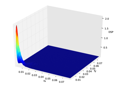
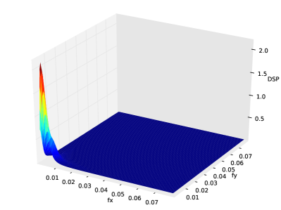
Figure 10: Case #1: (a) Average empirical periodogram of the stress field at $3.5\%$ macroscopic strain – (b) best fitted periodogram

Table 4 presents the results of the fitting of the average empirical periodogram calculated from 35 realizations of the field using three models, namely Gaussian, exponential and a mixed “Gaussian + exponential” as in Eq.(30).

Table 4: Fitted parameters and error estimates for the three fitted models: Gaussian, exponential and mixed “Gaussian + exponential”

Model	$\epsilon$	Gaussian					Exponential
	(Eq.(32))	$\sigma_{1}$	$l_{x1}$	$l_{y1}$	$f^{(1)}_{x0}$	$f^{(1)}_{y0}$	$\sigma_{2}$	$l_{x2}$	$l_{y2}$	$f^{(2)}_{x0}$	$f^{(2)}_{y0}$
Gaussian	$0.0043$	$69.4$	$104.6$	$102.9$	$0.00287$	$0$	$\_$	$\_$	$\_$	$\_$	$\_$
Exponential	$0.0039$	$\_$	$\_$	$\_$	$\_$	$\_$	$84.2$	$73.8$	$87.5$	$0.00275$	$0$
Mixed	$0.0017$	$54.7$	$138.4$	$159.1$	$0.00244$	$0$	$57.6$	$57.5$	$63.5$	$0.00562$	$0.0028$

From the results in Table 4 it appears that the mixed model provides a significantly smaller least-square error than that obtained from the Gaussian and exponential models respectively. The corresponding fitted periodogram is plotted in Figure 10-b.

In order to better appreciate the quality of the fitting, two-dimensional cuts of the empirical (resp. fitted) periodogram are given in Figures 11–13. Figure 11 corresponds to a cut along the $X$ direction for two values of $f_{y}=0\,;\,0.0013$. Figure 12 corresponds to a cut along the $Y$ direction for two values of $f_{x}=0\,;\,0.0013$. Finally Figure 13 corresponds to a cut along the diagonal $f_{x}=f_{y}$.

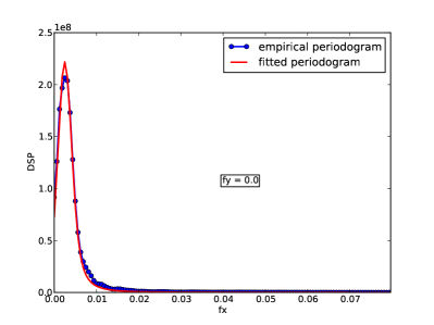
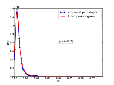
Figure 11: Case #1: Cut of the periodograms in the $X$ direction

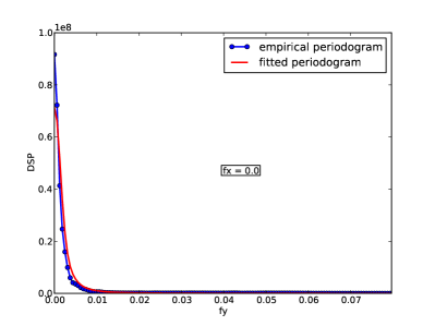
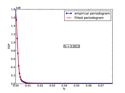
Figure 12: Case #1: Cut of the periodograms in the $Y$ direction

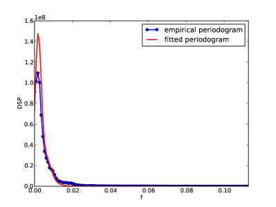
Figure 13: Case #1: Cut of the periodograms along the diagonal $f_{x}=f_{y}$

From the above figures it appears that the fitting of the empirical periodogram by a mixed model is remarkably accurate. It is interesting to interpret the fitted parameters reported in Table 4. First it is observed that the amplitude of each component of the mixed periodogram is similar since $\sigma_{1}\approx\sigma_{2}$. The variance of the field is equal to $\sigma_{1}^{2}+\sigma_{2}^{2}\approx$ 6,309 MPa². The associated standard deviation is 79.4 MPa. As the mean principal stress is 720 MPa at 3.5% macroscopic strain, the coefficient of variation of the field is about 11%.

In order to interpret the correlation length parameters let us define the mean size of a grain $S_{g}$ such a two-dimensional aggregate. As the volume of edge length equal to 1,000 corresponds to 100 grains, the equivalent diameter of a single grain reads:

$$D_{g}=\sqrt{\frac{4}{\pi}S_{g}}=\sqrt{\frac{4}{\pi}\frac{1,000\times 1,000}{100}}=112.8$$ (33)

Thus the correlation lengths obtained from the fitting vary from 0.55 to 1.3$D_{g}$. This shows that the characteristic dimension of the underlying microstructure (i.e. $D_{g}$) is of the same order of magnitude as these parameters. In other words the scale of local fluctuation of the stress field is related to the grain size, as heuristically expected. Moreover, it appears that the lengths in the $X$ and $Y$ directions are almost identical. The stress field does not show any significant anisotropy in this case.

5.3 Influence of the number of realizations

In this section the stability of the fitted parameters as a function of the number of available realizations $K$ used in the average periodogram method is considered. In practice the procedure applied in the previous paragraph is run using $K=8,9,\,\dots\,,35$ realizations of the stress field. The evolution of the standard deviations $(\sigma_{1},\sigma_{2})$ is shown in Figure 14. The evolution of the correlation lengths $l_{(x,y)(1,2)}$ is shown in Figure 15. The evolution of the initial frequencies $f_{(x,y)_{0}}^{(1,2)}$ is shown in Figure 16.

Figure 14: Case #1: Evolution of the fitted standard deviations with respect to the number of realizations $K=8,\,\dots\,,35$

Figure 15: Case #1: Evolution of the fitted correlation lengths in the $X,Y$ directions with respect to the number of realizations $K=8,\,\dots\,,35$

Figure 16: Case #1: Evolution of the fitted initial frequency in the $X,Y$ directions with respect to the number of realizations $K=8,\,\dots\,,35$

From these figures it appears that the fitted parameters tend to a converged value when at least 20 realizations of the stress field are used for their estimation.

5.4 Influence of the macroscopic strain level

In this section the evolution of the parameters of the fitted periodograms as a function of the macroscopic strain is investigated. For this purpose the methodology presented in Section 5.2 is applied using the realizations of the maximal principal stress fields corresponding to various levels of the loading curve, i.e. various values of the equivalent macroscopic strain $E_{YY}=0.,\,\dots\,,3.5\%$.

Figure 17: Case #1: Evolution of the fitted standard deviations with respect to the load level (macroscopic strain $E_{YY}=0.,\,\dots\,,3.5\%$)

The evolution of the standard deviations $(\sigma_{1},\sigma_{2})$ is shown in Figure 17. The two components of the periodogram (e.g. Gaussian and exponential) contribute for approximately the same proportion to the total variance of the field since the curves are almost superimposed. Note that these standard deviations increase with the applied load in the same way as the mean load curve (Figure 5).

The evolution of the correlation lengths $l_{(x,y)(1,2)}$ is shown in Figure 18. The evolution of the initial frequencies $f_{(x,y)_{0}}^{(1,2)}$ is shown in Figure 19. It is observed that once plasticity is settled (i.e. once the macroscopic strain $E_{YY}$ is greater than $\sim 0.5\%$) the parameters describing the fluctuations of the maximal principal stress field are almost constant. This conclusion is valid for both the correlation lengths and the initial frequencies. Note that the convergence is faster for the parameters related to the $X$ direction, i.e. the direction that is transverse to the one-dimensional loading. Finally it is also observed that $f^{(1)}_{y0}$ is almost equal to zero whatever the load level, thus the zero value in Table 4.

Figure 18: Case #1: Evolution of the fitted correlation lengths in the $X,Y$ directions with respect to the load level (macroscopic strain $E_{YY}=0.,\,\dots\,,3.5\%$)

Figure 19: Case #1: Evolution of the fitted initial frequency in the $X,Y$ directions with respect to the load level (macroscopic strain $E_{YY}=0.,\,\dots\,,3.5\%$)

6 Results – Case #2: random grain geometry

In this section both the randomness in the grain geometry and in the crystallographic orientations are taken into account. A total number of 35 finite element models are run. In each case, the grain geometry is obtained from a uniform sampling of points from which a Voronoï tessellation is built.

6.1 Check of the homogeneity

As in Section 5 the homogeneity of the maximal principal stress field is checked using the methodology proposed in Section 4.2. Figure 20 shows the evolution of $CV_{\mu_{K}}$ and $CV_{\sigma_{K}^{2}}$. These quantities regularly decrease and it is seen that they would tend to zero if a larger number of realizations was available. This leads to accepting the assumption that the random field is homogeneous.

Figure 20: Case #2: Evolution of $CV_{\mu_{K}}$ and $CV_{\sigma}^{K}$ with respect to the number of realizations

6.2 Identification of periodograms at 3.5% macroscopic strain

The average empirical periodogram obtained from $L=35$ realizations of the maximal principal stress field $\sigma_{I}$ at 3.5% of macroscopic strain is plotted in Figure 22-a. Three types of theoretical periodograms have been fitted as in the previous section, which lead to the conclusion that the mixed model that combines a Gaussian and an exponential component is best suited. The fitted parameters are gathered in Table 5 where the parameters fitted for Case #1 are also recalled for the sake of comparison.

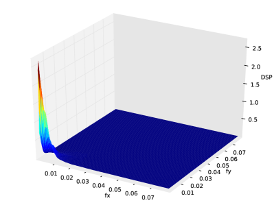
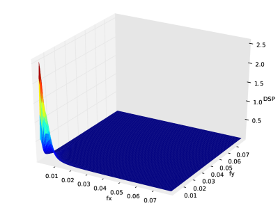
Figure 21: Case #2: (a) Average empirical periodogram of the stress field at $3.5\%$ macroscopic strain – (b) best fitted periodogram

In order to check the accuracy of the fitting, two-dimensional cuts of the empirical (resp. fitted periodogram) are plotted in Figure 22 (cut along the $X$ direction), Figure 23 (cut along the $Y$ direction), Figure 24 (cut along the diagonal $f_{x}=f_{y}$ ). Again the fitting is remarkably accurate, meaning that the fitted model of periodogram accurately represents the spatial variability of the maximal principal stress field.

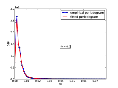
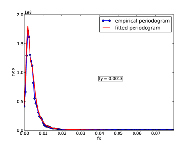
Figure 22: Case #2: Cut of the periodograms in the $X$ direction

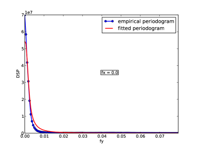
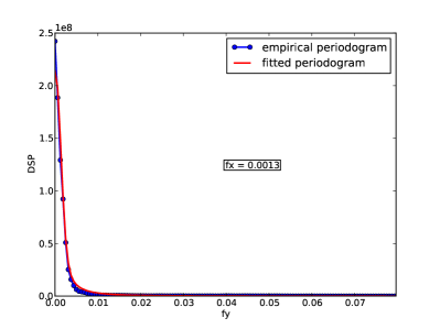
Figure 23: Case #2: Cut of the periodograms in the $Y$ direction

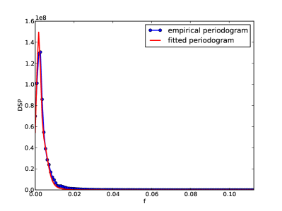
Figure 24: Case #2: Cut of the periodograms along the diagonal $f_{x}=f_{y}$

It can be observed from the figures in Table 5 that the fitting is of equal quality in both cases (relative error less than $2\,10^{-3}$). As far as the contribution of each component of the periodogram is concerned, the symmetry reported in Case #1 is not existing anymore since the standard deviation of the exponential contribution ($\sigma_{2}=81.6$) is much greater than that of the Gaussian part ($\sigma_{1}=35.8$). The total variance of the field is 7940 MPA², corresponding to a standard deviation of 89.1 MPa and a coefficient of variation of 12%. Thus there is a little more scattering in the random stress field obtained in Case #2 when considering both the random grain geometry and orientations.

Table 5: Fitted parameters and error estimates for the mixed “Gaussian + exponential” periodogram

Case	$\epsilon$	Gaussian					Exponential
	(Eq.(32))	$\sigma_{1}$	$l_{x1}$	$l_{y1}$	$f^{(1)}_{x0}$	$f^{(1)}_{y0}$	$\sigma_{2}$	$l_{x2}$	$l_{y2}$	$f^{(2)}_{x0}$	$f^{(2)}_{y0}$
Case #1	$0.0017$	$54.7$	$138.4$	$159.1$	$0.00244$	$0$	$57.6$	$57.5$	$63.5$	$0.00562$	$0.0028$
Case #2	$0.0018$	$35.8$	$269.5$	$174.5$	$0.00172$	$0$	$81.6$	$67.2$	$70.4$	$0.004$	$0$

The correlation lengths associated with the exponential part do not differ much in Case #2 compared to Case #1 (corresponding here to 1.5 to 2.4 $D_{g}$). In contrast the correlation lengths related to the Gaussian part are increased, which tends to produce less rapidly varying realizations. This may be explained by the fact that the grain boundaries are “averaged” in Case #2 whereas they were fixed in Case #1. The stress concentrations that are usually observed at the grain boundaries are thus smoothed in Case #2 compared to Case #1.

6.3 Influence of the number of realizations

In this section one considers the stability of the fitted parameters as a function of the number of available realizations $K$ used in the average periodogram method. The procedure applied in the previous paragraph is run using $K=8,9,\,\dots\,,35$ realizations of the stress field. The evolution of the standard deviations $(\sigma_{1},\sigma_{2})$ and the initial frequencies $f_{(x)_{0}}^{(1,2)}$ is shown in Figure 25 (note that $f_{(y)_{0}}^{(1,2)}=0$ in the present case). The evolution of the correlation lengths $l_{(x,y)(1,2)}$ is shown in Figure 26.

Figure 25: Case #2: Evolution of the fitted standard deviations and the initial frequencies $f_{(x)_{0}}^{(1,2)}$ with respect to the number of realizations $K=8,\,\dots\,,35$

Figure 26: Case #2: Evolution of the fitted correlation lengths in the $X$ (left) (resp. $Y$ (right)) directions with respect to the number of realizations $K=8,\,\dots\,,35$

From these figures it clearly appears that the fitted parameters are almost constant when the number of realizations of the stress field used in their estimation increases. The minimal number of $K=8$ could be used here without significant errors although it is recommended to keep a value of $K=20$ as in Case #1 for robustness.

6.4 Influence of the macroscopic strain level

Finally the evolution of the parameters of the fitted periodograms as a function of the macroscopic strain $E_{YY}$ is investigated. For this purpose the identification method is applied using the realizations of the maximal principal stress fields corresponding to various levels of the loading curve, i.e. various values of the equivalent macroscopic strain $E_{YY}=0.,\,\dots\,,3.5\%$.

Figure 27: Case #2: Evolution of the fitted standard deviations (left) with respect to the load level (macroscopic strain $E_{YY}=0.,\,\dots\,,3.5\%$) (resp. the initial frequencies $f_{(x,y)_{0}}^{(1)}$ (right))

Figure 28: Case #2: Evolution of the fitted correlation lengths in the $X$ (left) (resp. $Y$ (right)) directions with respect to the load level (macroscopic strain $E_{YY}=0.,\,\dots\,,3.5\%$)

The evolution of the two standard deviations look similar to the results obtained in Case #1 (Figure 27). It is observed that the ratio $\sigma_{2}/\sigma_{1}$ is almost constant all along the loading path up to 3.5% strain. As far as the initial frequencies are concerned, there is a complete independance with the load level as soon as $E_{YY}$ is greater than $\sim 0.5\%$, i.e. when plasticity has settled in the aggregate. The same conclusion can be drawn for the various correlation lengths.

7 Conclusions

The distribution of stresses in a material at a microscopic scale (where heterogeneities such as grain structures are taken into account) has been given much attention in the context of computational homogenization methods. However the current methods usually stick to a deterministic formulation. Starting from the premise that any representative volume element (such as a polycrystalline aggregate) is a single specific realization of a random quantity, the present paper aims at using methods of computational stochastic mechanics for representing the (random) stress field.

After recalling the basic mathematics of Gaussian random fields, the paper presents a periodogram method for estimating the parameters describing the spatial fluctuation of a random field from a collection of realizations of this field. This method is adapted in two dimensions from well-known techniques originating from signal processing.

The material under consideration, namely the 16MND5 steel used in nuclear pressure vessels is then presented together with a local modelling by polycrystalline finite element calculations. From a collection of 35 realizations of the (maximal principal) stress field, the spatial correlation structure of the latter is identified. By fitting various theoretical periodograms, a mixed model combining a Gaussian and an exponential-type contribution is retained. These two contributions may be empirically interpreted as follows: The Gaussian part corresponds to the fluctuation from grain to grain ; the (less smooth) exponential component corresponds to the sharp grain boundaries stress concentrations.

Two cases are considered, namely a “fixed-geometry” case in which only the crystallographic orientations changes within the 35 realizations (fixed grain boundaries), and a “variable geometry” in which the grain geometry is randomly sampled for each realization. In both cases, a good convergence of the procedure is observed when the number of realizations increases. A set of 20 realizations is recommended, although good results are already obtained for $\sim$8 realizations in Case #2.

Moreover it is shown that the correlation lengths are of the same order of magnitude as the grain size. The initial frequencies that are required for a best fitting of the periodogram and that translate into some kind of spatial periodicity in the covariogram could be explained by spurious edge effects due to the limited size of the aggregate. This should be investigated more in details in further analysis.

Another important result is drawn from the comparison of the fitted parameters at various load levels. Once plasticity is settled within the aggregate, the parameters describing the spatial fluctuations of the field are almost constant. Moreover the variance of the field (sum of the variance of each component of the periodogram) increases proportionally to the mean strain/stress curve, meaning that the coefficient of variation of the stress field is almost constant (around 11% for the fixed geometry and 12% for the variable geometry).

The results presented in this paper should be confirmed by additional investigations under different types of loading (e.g. biaxial loading). The tools that are presented here may be applicable to three-dimensional aggregates and stress fields at a much larger computational cost though. This work is currently in progress.

The identified stress fields may eventually be re-simulated: new realizations of the stress fields are straightforwardly obtained at a low computational cost by random field simulation techniques such as the spectral approach or the circulant embedding method (Preumont, 1990; Dang et al, 2011a, b). This allow us to apply local approach to fracture analysis (such as that presented in Mathieu et al (2006)) for the assessment of the brittle fracture of metallic materials, as shown in Dang et al (2013).

Acknowledgements
The second author is funded by a CIFRE grant at Phimeca Engineering S.A. subsidized by the French Agence Nationale de la Recherche et de la Technologie (convention number 027/2010). The research project is supported by EDF R&D under contract #8610-AAP5910056413. These supports are gratefully acknowledged.

References

- Arwade and Grigoriu (2004) Arwade S, Grigoriu M (2004) Probabilistic model for polycrystalline microstructures with application to intergranular fracture. J Eng Mech (ASCE) 130:997–1005
- Barber et al (1996) Barber C, Dobkin D, Huhdanpaa H (1996) The Quickhull algorithm for convex hulls. ACM Trans Math Software 22(4):469–483
- Beremin (1983) Beremin F (1983) A local criterion for cleavage fracture of a nuclear pressure vessel steel. Metal Trans 14A:2277–2287
- Chakraborty and Rahman (2008) Chakraborty A, Rahman S (2008) Stochastic multiscale models for fracture analysis of functionally graded materials. Eng Fract Mech 75(8):2062–2086
- Chung et al (2005) Chung D, Gutiérrez M, de Borst R (2005) Object-oriented stochastic finite element analysis of fibre metal laminates. Comput Methods Appl Mech Engrg 194(12-16):1427–1446
- Cramer and Leadbetter (1967) Cramer H, Leadbetter M (1967) Stationary and related processes. Wiley & Sons
- Dang et al (2011a) Dang H, Sudret B, Berveiller M, Zeghadi A (2011a) Identification of random stress fields from the simulation of polycrystalline aggregates. In: Proc. 1st Int. Conf. Computational Modeling of Fracture and Failure of Materials and Structures (CFRAC), Barcelona, Spain
- Dang et al (2011b) Dang HX, Sudret B, Berveiller B (2011b) Benchmark of random fields simulation methods and links with identification methods. In: Faber M, Köhler J, Nishijima K (eds) Proc. 11th Int. Conf. on Applications of Stat. and Prob. in Civil Engineering (ICASP11), Zurich, Switzerland
- Dang et al (2013) Dang HX, Berveiller M, Zeghadi A, Sudret B, Yalamas T (2013) Introducing stress random fields of polycrystalline aggregates into the local approach to fracture. Proc. 11th Int. Conf. Struct. Safety and Reliability (ICOSSAR’2013), Deodatis, G. (Ed.), New York, USA, 2013
- Franciosi (1985) Franciosi P (1985) The concepts of latent hardening and strain hardening in metallic single crystals. Acta Metall 33(9):1601–1612
- Gilbert (1962) Gilbert E (1962) Random subdivisions of space into crystals. Ann Math Stat 33(3):958–972
- Graham and Baxter (2001) Graham L, Baxter S (2001) Simulation of local material properties based on moving-window GMC. Prob Eng Mech 16(4):295–305
- Graham-Brady et al (2006) Graham-Brady L, Arwade S, Corr D, Gutiérrez M, Breysse D, Grigoriu M, Zabaras N (2006) Probability and materials: from nano- to macro-scale – a summary. Prob Eng Mech 21(3):193–199
- Grigoriu (2010) Grigoriu M (2010) Nearest neighbor probabilistic model for aluminum polycrystals. J Eng Mech (ASCE) 136:821–829
- Kouchmeshky and Zabaras (2009) Kouchmeshky B, Zabaras N (2009) The effect of multiple sources of uncertainty on the convex hull of material properties of polycrystals. Comput Mat Sci 47(2):342–352
- Kouchmeshky and Zabaras (2010) Kouchmeshky B, Zabaras N (2010) Microstructure model reduction and uncertainty quantification in multiscale deformation processes. Comput Mat Sci 48(2):213–227
- Laug and Borouchaki (1999) Laug P, Borouchaki H (1999) BLSURF-mesh generator for composite parametric surface. Tech. Rep. 0235, INRIA, user’s Manual
- Lautensack and Zuyev (2008) Lautensack C, Zuyev S (2008) Random Laguerre tessellations. Adv Appl Prob 40:630–658
- Leonardia et al. (2012) Leonardia A, Scardia P, Leonia M (2012) Realistic nano-polycrystalline microstructures: beyond the classical Voronoi tessellation. Phil Magazine 92(8):986–1005
- Li (2005) Li J (2005) Spectral estimation. Dep. of Electrical and Computer Engineering – University of Florida
- Li et al (2010) Li Z, Wen B, Zabaras N (2010) Computing mechanical response variability of polycrystalline microstructures through dimensionality reduction techniques. Comput Mat Sci 49(3):568–581
- Liu et al (2007) Liu H, Arwade S, Igusa T (2007) Random composites characterization using a classifier model. J Eng Mech (ASCE) 133:129–137
- Marquardt (1963) Marquardt D (1963) An algorithm for least-squares estimation of nonlinear parameters. J Soc Indus Appl Math 11(2):431–441
- Mathieu (2006) Mathieu J (2006) Analyse et modélisation micromécanique du comportement et de la rupture fragile de l’acier 16MND5: prise en compte des hétérogénéités microstructurales. PhD thesis, École Nationale Supérieure des Arts et Métiers
- Mathieu et al (2006) Mathieu J, Berveiller S, Inal K, Diard O (2006) Microscale modelling of cleavage fracture at low temperatures: influence of heterogeneities at the granular scale. Fatigue Fract Eng Mat Struct 29(9-10):725–737
- Mathieu et al (2010) Mathieu J, Inal K, Berveiller S, Diard O (2010) A micromechanical interpretation of the temperature dependence of Beremin model parameters for French RPV steel. J Nucl Mat 406(1):97–112
- Meric and Cailletaud (1991) Meric L, Cailletaud G (1991) Single crystal modelling for structural calculation : Part 2 - F.E. implementation. J Eng Mat Tech 113:171–182
- Perrin et al. (2014) Perrin G, Soize C, Duhamel D, Funfschilling (2014) A posteriori error and optimal reduced basis for stochastic processes defined by a finite set of realizations. SIAM/ASA J. Uncertainty Quantification, 2(1):745–762
- Preumont (1990) Preumont A (1990) Vibrations aléatoires et analyse spectrale. Presses polytechniques et universitaires romandes
- Stefanou (2009) Stefanou G (2009) The stochastic finite element method: Past, present and future. Comput Methods Appl Mech Engrg 198:1031–1051
- Stoica and Moses (1997) Stoica P, Moses R (1997) Introduction to spectral analysis. Prentice Hall
- Tanguy (2001) Tanguy B (2001) Modélisation de l’essai Charpy par l’approche locale de la rupture – application au cas de l’acier 16MND5 dans le domaine de la transition. PhD thesis, École des Mines ParisTech
- Vanmarcke (1983) Vanmarcke E (1983) Random fields : analysis and synthesis The MIT Press, Cambridge, Massachussets
- Xu and Chen (2009) Xu XF and Chen X (2009) Stochastic homogenization of random elastic multi-phase composites and size quantification of representative volume element. Mechanics of Materials, 41:174–186
- Zhang et al. (2011) Zhang P, Balint D, Lin J (2011) Controlled Poisson Voronoi tessellation for virtual grain structure generation: a statistical evaluation. Phil. Magazine 91(36), 4555–4573