Kohn-Luttinger superconductivity in monolayer and bilayer semimetals with the Dirac spectrum

Abstract

The effect of Coulomb interaction in an ensemble of Dirac fermions on the formation of superconducting pairing in monolayer and bilayer doped graphene is studied using the Kohn-Luttinger mechanism disregarding the Van der Waals potential of the substrate and impurities. The electronic structure of graphene is described using the Shubin-Vonsovsky model taking into account the intratomic, interatomic, and interlayer (in the case of bilayer graphene) Coulomb interactions between electrons. The Cooper instability is determined by solving the Bethe-Saltpeter integral equation. The renormalized scattering amplitude is obtained with allowance for the Kohn-Luttinger polarization contributions up to the second order of perturbation theory in the Coulomb interaction. It plays the role of effective interaction in the Bethe-Salpeter integral equation. It is shown that the allowance for the Kohn-Luttinger renormalizations as well as intersite Coulomb interaction noticeably affects the competition between the superconducting phases with the $f-$wave and $d+id-$wave symmetries of the order parameter. It is demonstrated that the superconducting transition temperature for an idealized graphene bilayer with significant interlayer Coulomb interaction between electrons is noticeably higher than in the monolayer case.

1 INTRODUCTION

Graphene is of considerable interest for fundamental physics and for applications due to its peculiar transport, pseudorelativistic, and quantum-electrodynamic properties  [1, 2, 3]. This combination of graphene properties is primarily determined by its unique gapless energy structure consisting of cone-shaped valence and conduction bands contacting at the corners of the first Brillouin zone (Dirac points) [4]. It has been established that electrons propagating in graphene near Dirac points resemble massless fermions with linear dispersion [5] and are characterized by the minimal conductivity for a zero charge carrier concentration [5, 6], a high mobility [7, 8, 9], Klein tunneling [10, 11], oscillating motion (Zitterbewegung) [12, 13], universal absorption of light [14], and many other properties having no analogs in other physical systems.

When in contact with superconductors, graphene exhibits exotic superconducting properties [15]. In spite of the fact that the evolution of the Cooper instability in graphene itself has not yet been confirmed, experimental evidence [16, 17, 18, 19, 20, 21] that graphene in contact with conventional superconductors exhibits superconducting properties have been obtained. The fact that short graphene samples placed between superconducting contacts can be used to construct Josephson junctions indicates that Cooper pairs can propagate coherently in graphene. In this connection, it would be interesting to find out whether it is possible to modify graphene structurally or chemically to convert it into a magnet [22] or even into a real superconductor.

It is known theoretically that a model with conic dispersion requires the minimal intensity of the pairing interaction for the development of the Cooper instability [23]. In this connection, there have been several attempts to analyze theoretically possible achievement of the superconducting state in doped monolayer, as well as bilayer, graphene. The role of topological defects in achieving Cooper pairing in a graphene monolayer was studied in [24]. In [25], the phase diagram for spin-singlet superconductivity in a monolayer was constructed by Uchoa and Castro Neto in the mean field approximation, and the plasmon mechanism of superconductivity leading to low superconducting transition temperatures in the $s$-wave channel was studied for realistic electron concentration values. The possibility of inducing superconductivity in a graphene monolayer due to electron correlations was investigated in [26, 27].

The situation in which the Fermi level is near one of the van Hove singularities in the density of states of a graphene monolayer was considered in [28]. It is well known that these singularities can enhance magnetic and superconducting fluctuations [29]. In accordance with the scenario described in [29], the Cooper instability occurs due to strong anisotropy of the Fermi contour for van Hove filling $n_{vH}$, which in fact originates from the Kohn-Luttinger mechanism [30] proposed in 1965 and assuming the occurrence of superconducting pairing in systems with purely repulsive interaction [31, 32, 33]. It was noted in [28] that this mechanism can occur in graphene because the electron-electron scattering becomes strongly anisotropic; for this reason, a channel with attraction can be formed when there is a projection onto harmonics with a nontrivial angular dependence on the Fermi surface. According to the result obtained in [28], such the Cooper instability in an idealized graphene monolayer evolves predominantly in the $d-$wave channel and can be responsible for superconducting transition temperatures up to $T_{c}\sim 10\,K$ depending on the proximity of the chemical potential level to the van Hove singularity. An analogous conclusion was drawn in [34], where the Kohn-Luttinger superconductivity in the vicinity of the van Hove singularity in the graphene monolayer was studied by the renormalization group method.

The possibility of the competition and coexistence of the Pomeranchuk instability and the Kohn-Luttinger superconducting instability in a graphene monolayer was considered in [35]. In [36], it was found in experiments with a strongly doped monolayer using angle-resolved photoemission spectroscopy (ARPES) that multiparticle interactions substantially deform the Fermi surface, leading to an extended van Hove singularity at point $M$ of the hexagonal Brillouin zone. The features of the ground state were investigated theoretically, and the competition between the ferromagnetic and superconducting instabilities was analyzed. It was shown that in this competition, the tendency to superconductivity due to strong modulation of the effective interaction along the Fermi contour (i.e., due to electron-electron interactions alone) prevails. The superconducting instability evolves predominantly in the $f-$wave channel in this case [36]. The competition between the superconducting phase and the spin density wave phase at van Hove filling and near it in the monolayer was analyzed in [37] by the functionalization renormalization group method. It was found that for the band structure parameters and the Coulomb interactions obtained by ab initio calculations for graphene and graphite monolayers [38], superconductivity with the $d+id-$wave type of symmetry of the order parameter prevails in a large domain near the van Hove singularity, and a change in the related parameters may lead to a transition to the phase of the spin density wave. According to [37], far away from the van Hove singularity, the long-range Coulomb interactions change the form of the $d+id-$wave function of a Cooper pair and can facilitate superconductivity with the $f-$wave symmetry of the order parameter.

In accordance with the results obtained in [39], in the case of bilayer graphene, ferromagnetic instability in the vicinity of the van Hove singularities dominates over the Kohn-Luttinger superconductivity. However, the Coulomb interaction screening function in the bilayer was calculated earlier in [40] in the random phase approximation (RPA) in the doped and undoped regimes. It was found that the static polarization operator of the doped bilayer contains the Kohn anomaly much larger than in the case of a monolayer or a 2D electron gas. It is well known that the singular part of the polarization operator or the Kohn anomaly [41, 42, 43] facilitates effective attraction between two particles, ensuring a contribution that always exceeds the repulsive contribution associated with the regular part of the polarization operator for the orbital angular momenta $l\neq 0$ of the pair [30]. Thus, we can expect that the superconducting transition temperature $T_{c}$ in the idealized bilayer may exceed the corresponding value for the idealized monolayer.

In addition, it was shown in earlier publications [44, 45] that the value of $T_{c}$ can be increased via the Kohn- Luttinger mechanism even for low concentrations of charge carriers if we consider the spin-polarized or two-band situation, as well as a multilayer system. In this case, the role of the pairing spins up is played by electrons of the first band (layer), while the role of the screening spins down is played by electrons of the second band (layer). Coupling between the electrons of the two bands occurs via interband (interlayer) Coulomb interaction. As a result, the following superconductivity mechanism becomes possible: electrons of one species form a Cooper pair by polarizing electrons of another species [44, 45]. This mechanism of superconductivity is also effective in quasi-two-dimensional systems. Note that odd-momentum pairing and superconductivity in vertical graphene heterostructures made up by graphene layers separated by boron nitride spaces was considered recently by Guinea and Uchoa [25].

In this work, we investigate the Kohn-Luttinger Cooper instability in an idealized monolayer and bilayer of doped graphene using the Born weak-coupling approximation and taking into account the Coulomb repulsion between electrons of the same and of the nearest carbon atoms in a monolayer, as well as the interlayer Coulomb repulsion in the case of the bilayer.

The necessity of including the long-range Coulomb interaction in calculating the physical characteristics of graphene is dictated by the results obtained in  [38], where the partly screened frequency-dependent Coulomb interaction was calculated ab initio in constructing the effective multiparticle model of graphene and graphite. It was found that the intra-atomic repulsion potential in graphene is $U=9.3\,\textrm{eV}$ (an analogous estimate is given in [46]), which contradicts the intuitively expected small value of $U$ and weak-coupling limit $U<W$. The calculations performed in [38] have demonstrated the fundamental importance of taking into account the nonlocal Coulomb interaction in graphene: the Coulomb repulsion of electrons at neighboring sites amounts to $V=5.5\,\textrm{eV}$. It should be noted that the values of $U$ and $V$ estimated by other researchers (see, e.g., [47]) are much smaller.

2 IDEALIZED GRAPHENE MONOLAYER

In the hexagonal lattice of graphene, each unit cell contains two carbon atoms; therefore, the entire lattice can be divided into two sublattices $A$ and $B$. In the Shubin-Vonsovsky (extended Hubbard) model, the Hamiltonian for the graphene monolayer taking into account electron hoppings between the nearest and next-to-nearest atoms, as well as the Coulomb repulsion between electrons of the same atom and of adjacent atoms in the Wannier representation, has the form

$$\hat{H} = \hat{H}_{0}+\hat{H}_{\textrm{int}},$$ (1)

$$\hat{H}_{0} = -\mu\Biggl{(}\sum_{f\sigma}\hat{n}^{A}_{f\sigma}+\sum_{g\sigma}\hat{n}^{B}_{g\sigma}\Biggr{)}-$$

$$- t_{1}\sum_{f\delta\sigma}(a^{{\dagger}}_{f\sigma}b_{f+\delta,\sigma}+\textrm{h.c.})-$$

$$- t_{2}\Biggl{(}\sum_{\langle\langle fm\rangle\rangle}a^{{\dagger}}_{f\sigma}a_{m\sigma}+\sum_{\langle\langle gn\rangle\rangle}b^{{\dagger}}_{g\sigma}b_{n\sigma}+\textrm{h.c.}\Biggr{)},$$

$$\hat{H}_{\textrm{int}} = U\Biggl{(}\sum_{f}\hat{n}^{A}_{f\uparrow}\hat{n}^{A}_{f\downarrow}+\sum_{g}\hat{n}^{B}_{g\uparrow}\hat{n}^{B}_{g\downarrow}\Biggr{)}+$$ (3)

$$+ V\sum_{f\delta\sigma}\hat{n}^{A}_{f\sigma}\hat{n}^{B}_{f+\delta,\sigma}.$$

Here, operators $a^{{\dagger}}_{f\sigma}(a_{f\sigma})$ create (annihilate) an electron with spin projection $\sigma=\pm 1/2$ at site $f$ of sublattice $A$; $\displaystyle\hat{n}^{A}_{f\sigma}=a^{{\dagger}}_{f\sigma}a_{f\sigma}$ denotes the operators of the number of fermions at the $f$ site of sublattice $A$ (analogous notation is used for sublattice $B$). Vector $\delta$ connects the nearest atoms of the hexagonal lattice. In the Hamiltonian, the symbol $\langle\langle~{}\rangle\rangle$ indicates that summation is carried out only over next-to-nearest neighbors.

Passing to the momentum space and performing the Bogoliubov transformation,

$$\alpha_{i\textbf{k}\sigma}=w_{i1}(\textbf{k}){a_{\textbf{k}\sigma}}+w_{i2}(\textbf{k}){b_{\textbf{k}\sigma}},\qquad i=1,2,$$ (4)

we diagonalize Hamiltonian $\hat{H}_{0}$, which acquires the form

$$\hat{H}_{0}=\sum\limits_{i=1}^{2}\sum\limits_{\textbf{k}\sigma}E_{i\textbf{k}}{\alpha_{i\textbf{k}\sigma}^{{\dagger}}\alpha_{i\textbf{k}\sigma}}.$$ (5)

The two-band energy spectrum is described by the expressions [4]

$$E_{1\textbf{k}}=t_{1}|u_{\textbf{k}}|-t_{2}f_{\textbf{k}},\qquad E_{2\textbf{k}}=-t_{1}|u_{\textbf{k}}|-t_{2}f_{\textbf{k}},$$ (6)

where the following notation has been introduced:

$$f_{\textbf{k}}=2\cos(\sqrt{3}k_{y})+4\cos\biggl{(}\frac{\sqrt{3}}{2}k_{y}\biggr{)}\cos\biggl{(}\frac{3}{2}k_{x}\biggr{)},$$ (7)

$$u_{\textbf{k}}=\displaystyle\sum_{\delta}e^{i\textbf{k}\delta}=e^{-ik_{x}}+2e^{\frac{i}{2}k_{x}}\cos\biggl{(}\frac{\sqrt{3}}{2}k_{y}\biggr{)},$$ (8)

$$|u_{\textbf{k}}|=\sqrt{3+f_{\textbf{k}}}.$$ (9)

The coefficients of the Bogoliubov transformation have the form

$${w_{1,1}}(\textbf{k})=w_{22}^{*}(\textbf{k})=\frac{1}{\sqrt{2}}r_{\textbf{k}}^{*},\qquad r_{\textbf{k}}=\frac{u_{\textbf{k}}}{|u_{\textbf{k}}|},$$ (10)

$${w_{12}}(\textbf{k})=-w_{21}(\textbf{k})=-\frac{1}{\sqrt{2}}.$$

In the Bogoliubov representation, interaction operator (3) is defined by the following expression including operators $\alpha_{1\textbf{k}\sigma}$ and $\alpha_{2\textbf{k}\sigma}$: $\alpha_{1\textbf{k}\sigma}$ $\alpha_{2\textbf{k}\sigma}$

$$\hat{H}_{int} = \frac{1}{N}\sum\limits_{ijlm\atop\textbf{k}\textbf{p}\textbf{q}\textbf{s}\sigma}\Gamma_{ij;lm}^{||}(\textbf{k},\textbf{p}|\textbf{q},\textbf{s})\alpha_{i\textbf{k}\sigma}^{\dagger}\alpha_{j\textbf{p}\sigma}^{\dagger}\alpha_{l\textbf{q}\sigma}\alpha_{m\textbf{s}\sigma}\times$$

$$\times \Delta(\textbf{k}+\textbf{p}-\textbf{q}-\textbf{s})+$$

$$+ \frac{1}{N}\sum\limits_{ijlm\atop\textbf{k}\textbf{p}\textbf{q}\textbf{s}}\Gamma_{ij;lm}^{\bot}(\textbf{k},\textbf{p}|\textbf{q},\textbf{s})\alpha_{i\textbf{k}\uparrow}^{\dagger}\alpha_{j\textbf{p}\downarrow}^{\dagger}\alpha_{l\textbf{q}\downarrow}\alpha_{m\textbf{s}\uparrow}\times$$

$$\times \Delta(\textbf{k}+\textbf{p}-\textbf{q}-\textbf{s}),$$

where $\Delta$ is the Kronecker symbol, while $\Gamma_{ij;lm}^{||}(\textbf{k},\textbf{p}|\textbf{q},\textbf{s})$ and $\Gamma_{ij;lm}^{\bot}(\textbf{k},\textbf{p}|\textbf{q},\textbf{s})$ are the initial amplitudes. The quantity

$$\Gamma_{ij;lm}^{||}(\textbf{k},\textbf{p}|\textbf{q},\textbf{s}) = \frac{1}{2}\Bigl{(}V_{ij;lm}(\textbf{k},\textbf{p}|\textbf{q},\textbf{s})+$$ (12)

$$+ V_{ji;ml}(\textbf{p},\textbf{k}|\textbf{s},\textbf{q})\Bigr{)},$$

$$V_{ij;lm}(\textbf{k},\textbf{p}|\textbf{q},\textbf{s}) = V{u_{\textbf{q}-\textbf{p}}}w_{i1}(\textbf{k})w_{j2}(\textbf{p})w^{*}_{l2}(\textbf{q})w^{*}_{m1}(\textbf{s})$$

describes the intensity of the interaction of fermions with parallel spin projections, while the quantity

$$\Gamma_{ij;lm}^{\bot}(\textbf{k},\textbf{p}|\textbf{q},\textbf{s})=U_{ij;lm}(\textbf{k},\textbf{p}|\textbf{q},\textbf{s})+$$

$$\qquad\qquad+V_{ij;lm}(\textbf{k},\textbf{p}|\textbf{q},\textbf{s})+V_{ji;ml}(\textbf{p},\textbf{k}|\textbf{s},\textbf{q}),$$ (14)

$$U_{ij;lm}(\textbf{k},\textbf{p}|\textbf{q},\textbf{s})=U\Bigl{(}w_{i1}(\textbf{k})w_{j1}(\textbf{p})w^{*}_{l1}(\textbf{q})w^{*}_{m1}(\textbf{s})+$$

$$\qquad\qquad+w_{i2}(\textbf{k})w_{j2}(\textbf{p})w^{*}_{l2}(\textbf{q})w^{*}_{m2}(\textbf{s})\Bigr{)}$$ (15)

corresponds to the interaction of Fermi quasiparticles with antiparallel spin projections. Indices ${i,j,l,m}$ can acquire values of 1 or 2.

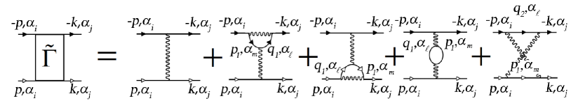
Figure 1: Fig. 1. First- and second-order diagrams for the effective interaction of electrons in graphene monolayer and bilayer. Solid lines with light (dark) arrows correspond to the Green s functions for electrons with spin projections $+{\textstyle{1\over 2}}$ ($-{\textstyle{1\over 2}}$) and energies corresponding to graphene energy bands $\alpha_{i}$, $\alpha_{j}$, $\alpha_{l}$ and $\alpha_{m}$. In diagrams for the monolayer (Section 2), subscripts $i=j=1$; subscripts $l$ and $m$ can acquire values of 1 or 2. In the case of the bilayer (Section 3), subscripts $i$ and $j$ acquire values of 1 or 2, while subscripts $l$ and $m$ acquire values of 1, 2, 3, or 4. Momenta $q_{1}$ and $q_{2}$ are defined by relations (19).

Using the Born weak coupling approximation (with the hierarchy $W>U>V$ of the model parameters, where $W$ is the bandwidth for the upper and lower branches of the energy spectrum (6) and (7) of graphene for the case of $t_{2}=0$), we can consider the scattering amplitude in the Cooper channel, confining our analysis to only second-order diagrams in the effective interaction of two electrons with opposite values of the momentum and spin and using quantity $\widetilde{\Gamma}(\textbf{p},\textbf{k})$ for it. Graphically, this quantity is determined by the sum of the diagrams shown in Fig. 1. Solid lines with light (dark) arrows correspond to Green s functions for electrons with opposite values of spin projections $+\frac{1}{2}~{}(-\frac{1}{2})$. It is well known that the possibility of Cooper pairing is determined by the characteristics of the energy spectrum near the Fermi level and by the effective interaction of electrons located near the Fermi surface [49]. Assuming that the chemical potential in doped graphene falls into the upper energy band $E_{1\textbf{k}}$ and analyzing the conditions for the occurrence of Kohn- Luttinger superconductivity, we can consider the situation in which the initial and final momenta also belong to the upper subband. This is reflected in Fig. 1 via indices $\alpha_{1}$ (upper band) and $\alpha_{2}$ (lower band).

The first diagram in Fig. 1 corresponds to the initial interaction of two electrons in the Cooper channel. The next (Kohn-Luttinger) diagrams in Fig. 1 describe second-order scattering processes, $\delta\widetilde{\Gamma}(\textbf{p},\textbf{k})$, and take into account the polarization effects of the filled Fermi sphere. Two solid lines without arrows in these diagrams indicate summation over both spin projections. Wavy lines correspond to the initial interaction. Scattering of electrons with identical spin projections corresponds only to the intersite contribution. If electrons with different spin projections interact, the scattering amplitude is determined by the sum of the Hubbard and intersite repulsions. Thus, in the presence of the short-range Coulomb interaction alone, the correction $\delta\widetilde{\Gamma}(\textbf{p},\textbf{k})$ to the effective interaction is determined by the last exchange diagram only. If the Coulomb interaction of electrons at neighboring lattice sites of graphene is taken into account, all diagrams in Fig. 1 contribute to the renormalized amplitude.

After the introduction of the analytical expressions for the diagrams, we obtain the following analytic expression for the effective interaction in Fig. 1:

$$\widetilde{\Gamma}(\textbf{p},\textbf{k})=\frac{U}{2}+\frac{V}{2}\textrm{Re}(u_{\textbf{p}-\textbf{k}}r^{*}_{\textbf{p}}r_{\textbf{k}})+\delta\widetilde{\Gamma}(\textbf{p},\textbf{k}),$$ (16)

where

$$\delta\tilde{\Gamma}(\textbf{p},\textbf{k})=\frac{1}{N}\sum\limits_{i,j,\textbf{p}_{1}}\Gamma^{\bot}_{1i;1j}(\textbf{p},\textbf{q}_{2}|-\textbf{k},\textbf{p}_{1})\times$$

$$\times\Gamma^{\bot}_{j1;i1}(\textbf{p}_{1},-\textbf{p}|\textbf{q}_{2},\textbf{k})\chi_{i,j}(\textbf{q}_{2},\textbf{p}_{1})+$$

$$+\frac{2}{N}\sum\limits_{i,j,\textbf{p}_{1}}\Bigl{\{}\Gamma^{\bot}_{1j;i1}(\textbf{p},\textbf{p}_{1}|\textbf{q}_{1},\textbf{k})\times$$

$$\times\left[\Gamma^{||}_{i1;j1}(\textbf{q}_{1},-\textbf{p}|\textbf{p}_{1},-\textbf{k})-\Gamma^{||}_{i1;1j}(\textbf{q}_{1},-\textbf{p}|-\textbf{k},\textbf{p}_{1})\right]\Bigr{.}+$$

$$+\Bigl{.}\Gamma^{\bot}_{i1;1j}(\textbf{q}_{1},-\textbf{p}|-\textbf{k},\textbf{p}_{1})\times$$

$$\times\left[\Gamma^{||}_{1j;1i}(\textbf{p},\textbf{p}_{1}|\textbf{k},\textbf{q}_{1})-\Gamma^{||}_{1j;i1}(\textbf{p},\textbf{p}_{1}|\textbf{q}_{1},\textbf{k})\right]\Bigr{\}}\chi_{i,j}(\textbf{q}_{1},\textbf{p}_{1}).$$

Here, we have introduced the following notation for generalized susceptibilities:

$$\chi_{i,j}(\textbf{k},\textbf{p})=\frac{f(E_{i\textbf{k}})-f(E_{j\textbf{p}})}{E_{j\textbf{p}}-E_{i\textbf{k}}},$$ (18)

where

$$f(x)=(\exp(\frac{x-\mu}{T})+1)^{-1}$$

— is the Fermi-Dirac distribution function, and energies $E_{i\textbf{k}}$ are defined by expressions (6). For the sake of compactness, we have introduced the notation for the combinations of momenta:

$$\textbf{q}_{1}=\textbf{p}_{1}+\textbf{p}-\textbf{k},\qquad\textbf{q}_{2}=\textbf{p}_{1}-\textbf{p}-\textbf{k}.$$ (19)

Knowing the renormalized expression for the effective interaction, we can pass to analysis of the conditions for the emergence of superconductivity in the system under investigation. It is well known [49] that the emergence of Cooper instability can be established from analysis of the homogeneous part of the Bethe-Saltpeter equation. In this case, the dependence of the scattering amplitude $\Gamma(\textbf{p},\textbf{k})$ on momentum k can be factorized, which gives the integral equation for the superconducting order parameter $\Delta(\textbf{p})$. After integrating over isoenergetic contours, we can reduce the problem of the Cooper instability to the eigenvalue problem [50, 33, 51, 52, 53, 54]

$$\frac{3\sqrt{3}}{8\pi^{2}}\oint\limits_{\varepsilon_{\textbf{q}}=\mu}\frac{d\hat{\textbf{q}}}{v_{F}(\hat{\textbf{q}})}\widetilde{\Gamma}(\hat{\textbf{{p}}},\hat{\textbf{q}})\Delta(\hat{\textbf{q}})=\lambda\Delta(\hat{\textbf{p}}),$$ (20)

where superconducting order parameter $\Delta(\hat{\textbf{q}})$ plays the role of the eigenvector, and eigenvalues $\lambda$ satisfy the relation $\lambda^{-1}\simeq\ln(T_{c}/W)$. In this case, momenta $\hat{\textbf{p}}$ and $\hat{\textbf{q}}$ lie on the Fermi surface and $v_{F}(\hat{\textbf{q}})$ is the Fermi velocity.

To solve Eq. (20), we write its kernel as the superposition of eigenfunctions each of which belongs to one of irreducible representations of symmetry group $C_{6v}$ of the hexagonal lattice. It is well known that this symmetry group has six irreducible representations  [55]: four 1D and two 2D representations. For each representation, Eq. (20) has a solution with its own effective coupling constant . We will henceforth use the following notation for the classification of the order parameter symmetries: representation $A_{1}$ corresponds to the $s-$wave symmetry type; $B_{1}$ and $B_{2}$ correspond to the $f-$wave symmetry; $E_{1}$, to the $p+ip-$wave symmetry type; and $E_{2}$, to the $d+id-$wave symmetry type.

For each irreducible representation $\nu$, we will seek the solution to Eq. (20) in the form

$$\Delta^{(\nu)}(\phi)=\sum\limits_{m}\Delta_{m}^{(\nu)}g_{m}^{(\nu)}(\phi),$$ (21)

where $m$ is the number of the eigenfunction belonging to representation $\nu$ and $\phi$ is the angle determining the direction of momentum $\hat{\textbf{p}}$ relative to the $p_{x}$ axis. The explicit form of the orthonormal functions $g_{m}^{(\nu)}(\phi)$ is defined by the expressions

$$A_{1} \rightarrow~{}g_{m}^{(s)}(\phi)=\frac{1}{\sqrt{(1+\delta_{m0})\pi}}\,\textrm{cos}\,6m\phi,~{}~{}m\in[\,0,\infty),$$

$$A_{2} \rightarrow~{}g_{m}^{(A_{2})}(\phi)=\frac{1}{\sqrt{\pi}}\,\textrm{sin}\,(6m+6)\phi,$$

$$B_{1} \rightarrow~{}g_{m}^{(f_{1})}(\phi)=\frac{1}{\sqrt{\pi}}\,\textrm{sin}\,(6m+3)\phi,$$ (22)

$$B_{2} \rightarrow~{}g_{m}^{(f_{2})}(\phi)=\frac{1}{\sqrt{\pi}}\,\textrm{cos}\,(6m+3)\phi,$$

$$E_{1} \rightarrow~{}g_{m}^{(p+ip)}(\phi)=\frac{1}{\sqrt{\pi}}\,(A\,\textrm{sin}\,(2m+1)\phi+$$

$$\qquad+B\,\textrm{cos}\,(2m+1)\phi),$$

$$E_{2} ~{}\rightarrow~{}g_{m}^{(d+id)}(\phi)=\frac{1}{\sqrt{\pi}}\,(A\,\textrm{sin}\,(2m+2)\phi+$$

$$\qquad+B\,\textrm{cos}\,(2m+2)\phi).$$

Here, subscripts $m$ for the 2D representations $E_{1}$ and $E_{2}$ run through the values for which coefficients $(2m+1)$ and $(2m+2)$, respectively, are not multiples of three.

The basis functions satisfy the orthonormality conditions

$$\int\limits_{0}^{2\pi}d\phi\,g_{m}^{(\nu)}(\phi)g_{n}^{(\beta)}(\phi)=\delta_{\nu\beta}\delta_{mn}.$$ (23)

Substituting expression (21) into Eq. (20), integrating with respect to angles, and using condition (23), we obtain

$$\sum_{n}\Lambda^{(\nu)}_{mn}\Delta_{n}^{(\nu)}=\lambda_{\nu}\Delta_{m}^{(\nu)},$$ (24)

where

$$\Lambda^{(\alpha)}_{mn} = \frac{3\sqrt{3}}{8\pi^{2}}\oint\limits_{0}^{2\pi}d\phi_{\textbf{p}}\oint\limits_{0}^{2\pi}d\phi_{\textbf{q}}\frac{d\hat{\textbf{q}}}{d\phi_{\textbf{q}}v_{F}(\hat{\textbf{q}})}\widetilde{\Gamma}({\hat{\textbf{p}}}\,|{\hat{\textbf{q}}})\times$$ (25)

$$\times g_{m}^{(\nu)}(\phi_{\textbf{p}})g_{n}^{(\nu)}(\phi_{\textbf{q}}).$$

Since $T_{c}\sim W\exp\bigl{(}1/\lambda\bigr{)}$, each negative eigenvalue $\lambda_{\nu}$ corresponds to the superconducting phase with the order parameter symmetry $\nu$. Generally speaking, the expansion of the order parameter $\Delta^{(\nu)}(\phi)$ in eigenfunctions includes a large number of harmonics; however, the main contribution is determined by only some of these harmonics. The highest value of the superconducting transition temperature corresponds to the modulus of the largest value of $\lambda_{\nu}$.

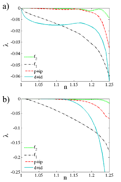
Figure 2: Fig. 2. Dependences of $\lambda$ on carrier concentration $n$ in the graphene monolayer: (a) $t_{2}=0,U=2|t_{1}|$, and $V=0$; (b) $t_{2}=0,U=2|t_{1}|$, and $V=0.5|t_{1}|$.

Figure 2a shows the calculated dependencies of the effective coupling constant $\lambda$ on carrier concentration $n$ for various symmetry types of the superconducting order parameter for the set of parameters $t_{2}=0,\,U=2|t_{1}|$, and $V=0$. It can be seen that for low electron densities $1<n<1.12$, in the vicinity of the van Hove singularity, the competition occurs between the superconducting phases with the $f-$wave symmetry type, whose contribution is determined by the harmonics $g_{m}^{(f_{1})}(\phi)=\displaystyle\frac{1}{\sqrt{\pi}}\,\textrm{sin}\,(6m+3)\phi$, and the $d+id-$wave symmetry type corresponding to 2D representation $E_{2}$. In the electron concentration range $1<n<1.12$, the $d+id-$wave pairing prevails, while for $1.12<n<n_{vH}$, superconductivity with the $f-$wave symmetry type of the order parameter is stabilized.

It should be noted that to avoid the summation of parquet diagrams [56, 57], we do not analyze here the electron concentration ranges which are too close to the van Hove singularity (Fig. 3).

The account of the intersite Coulomb interaction considerably affects the competition between superconducting phases. This can be seen from Fig. 2b which shows the $\lambda(n)$ dependences for parameters $t_{2}=0,U=2|t_{1}|$, and $V=0.5|t_{1}|$. Comparison with Fig. 2a shows that the switching of the intersite Coulomb interaction suppresses Cooper pairing in the $d+id$-wave channel for low electron densities; however, it leads to superconductivity with this type of symmetry in the vicinity of the van Hove singularity. As a result, the $f$-wave pairing takes place in the electron concentration range $1<n<1.22$. It should be noted that this result is in qualitative agreement with the results obtained in [37].

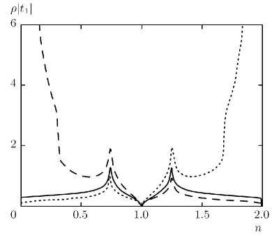
Figure 3: Fig. 3. Modification of the electron density of states for the graphene monolayer upon switching of the hoppings to the next-to-nearest atoms for $t_{2}=0$ solid curve), $t_{2}=-0.2|t_{1}|$ (dashed curve), and $t_{2}=0.2|t_{1}|$ (dotted curve).

The switching of electron hoppings $t_{2}$ to the next-to-nearest carbon atoms in the graphene monolayer does not qualitatively affect the competition between the superconducting phases of different symmetry types, which is illustrated in Fig. 2b [58]. Such a behavior of the system can be explained by the fact that an account of hoppings $t_{2}>0$ or $t_{2}<0$ does not noticeably modify the density of electron states of the monolayer in the range of carrier concentrations between the Dirac point and both van Hove singularities (Fig. 3). However, the inclusion of hoppings $t_{2}$ leads to an increase in the absolute values of the effective interaction and, hence, to higher superconducting transition temperatures in the idealized graphene monolayer [58].

3 IDEALIZED GRAPHENE BILAYER

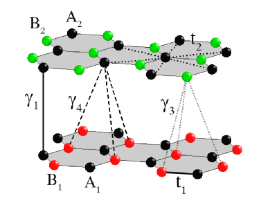
Figure 4: Fig. 4. Crystal structure of the graphene bilayer. Carbon atoms $A_{1}$ and $B_{1}$ in the lower layer are shown by red and black balls; atoms $A_{2}$ and $B_{2}$ in the upper layer are shown by black and green balls. Intralayer electron hoppings are marked by $t_{1}$ and $t_{2}$; $\gamma_{1},\,\gamma_{3}$, and $\gamma_{4}$ show the interplanar hoppings.

Let us consider an idealized graphene bilayer, assuming that two monolayers are arranged in accordance with the $AB$ type (i.e., one monolayer is turned through 60^o relative to the other monolayer) [59, 60]. We choose the arrangement of the sublattices in the layers in such a way that the sites from different layers located one above another belong to sublattice $A$, while the remaining sites belong to sublattice $B$ (Fig. 4). In this case, the Hamiltonian of the graphene bilayer in the Wannier representation has the form

$$\hat{H} = \hat{H}_{0}+\hat{H}_{\textrm{int}},$$ (26)

$$\hat{H}_{0} = (\varepsilon-\mu)\Biggl{(}\sum_{if\sigma}\hat{n}^{A}_{if\sigma}+\sum_{ig\sigma}\hat{n}^{B}_{ig\sigma}\Biggr{)}$$ (27)

$$- t_{1}\sum_{f\delta\sigma}(a^{{\dagger}}_{1f\sigma}b_{1,f+\delta,\sigma}+a^{{\dagger}}_{2f\sigma}b_{2,f-\delta,\sigma}+\textrm{h.c.})$$

$$- t_{2}\sum_{i\sigma}\Biggl{(}\sum_{\langle\langle fm\rangle\rangle}a^{{\dagger}}_{if\sigma}a_{im\sigma}+\sum_{\langle\langle gn\rangle\rangle}b^{{\dagger}}_{ig\sigma}b_{in\sigma}+\textrm{h.c.}\Biggr{)}$$

$$- \gamma_{1}\sum_{f\sigma}(a^{{\dagger}}_{1f\sigma}a_{2f\sigma}+\textrm{h.c.})-\gamma_{3}\sum_{g\delta\sigma}(b^{{\dagger}}_{1g\sigma}b_{2,g+\delta,\sigma}+\textrm{h.c.})$$

$$- \gamma_{4}\sum_{f\delta\sigma}(a^{{\dagger}}_{1f\sigma}b_{2,f-\delta,\sigma}+a^{{\dagger}}_{2f\sigma}b_{1,f+\delta,\sigma}+\textrm{h.c.}),$$

$$\hat{H}_{\textrm{int}} = U\biggl{(}\sum_{if}\hat{n}^{A}_{if\uparrow}\hat{n}^{A}_{if\downarrow}+\sum_{ig}\hat{n}^{B}_{ig\uparrow}\hat{n}^{B}_{ig\downarrow}\biggr{)}$$ (28)

$$+ V\sum_{f\delta\sigma}\Bigl{(}\hat{n}^{A}_{1f\sigma}\hat{n}^{B}_{1,f+\delta,\sigma}+\hat{n}^{A}_{2f\sigma}\hat{n}^{B}_{2,f-\delta,\sigma}\Bigr{)}$$

$$+ G_{1}\sum_{f\sigma}\hat{n}^{A}_{1f\sigma}\hat{n}^{A}_{2f\sigma}+G_{3}\sum_{g\delta\sigma}\hat{n}^{B}_{1g\sigma}\hat{n}^{B}_{2,g+\delta,\sigma}$$

$$+ G_{4}\sum_{f\delta\sigma}\Bigl{(}\hat{n}^{A}_{1f\sigma}\hat{n}^{B}_{2,f-\delta,\sigma}+\hat{n}^{A}_{2f\sigma}\hat{n}^{B}_{1,f+\delta,\sigma}\Bigr{)}.$$

Here, we have used notation analogous to that for Hamiltonian (1) for a monolayer in Section 2. Index $i=1,2$ in Hamiltonian (26) denotes the number of the monolayer. We assume that one-site energies are identical ($\varepsilon_{A1}=\varepsilon_{A2}=\varepsilon_{B1}=\varepsilon_{B2}=\varepsilon$). Interlayer electron hopping parameters are denoted by $\gamma_{1},\,\gamma_{3},\,\gamma_{4}$ (see Fig. 4). The last three terms in Hamiltonian (26) take into account the interlayer Coulomb interaction of electrons in atoms $A_{1}$ and $A_{2}$, $B_{1}$ and $B_{2}$, and $A_{1}$ and $B_{2}$; the intensities of these interactions are denoted by $G_{1}$, $G_{3}$, and $G_{4}$, respectively.

Passing to the momentum space, it is convenient to write Hamiltonian $\hat{H}_{0}$ in matrix form:

$$\hat{H}_{0}=$$ (29)

$$-\sum_{\textbf{k}\sigma}\left(\begin{array}[]{c}a^{{\dagger}}_{1\textbf{k}\sigma}\\ a^{{\dagger}}_{2\textbf{k}\sigma}\\ b^{{\dagger}}_{1\textbf{k}\sigma}\\ b^{{\dagger}}_{2\textbf{k}\sigma}\\ \end{array}\right)^{T}\left(\begin{array}[]{cccc}\varepsilon_{\textbf{k}}&\gamma_{1}&t_{1}u^{*}_{\textbf{k}}&\gamma_{4}u_{\textbf{k}}\\ \gamma_{1}&\varepsilon_{\textbf{k}}&\gamma_{4}u^{*}_{\textbf{k}}&t_{1}u_{\textbf{k}}\\ t_{1}u_{\textbf{k}}&\gamma_{4}u_{\textbf{k}}&\varepsilon_{\textbf{k}}&\gamma_{3}u^{*}_{\textbf{k}}\\ \gamma_{4}u^{*}_{\textbf{k}}&t_{1}u^{*}_{\textbf{k}}&\gamma_{3}u_{\textbf{k}}&\varepsilon_{\textbf{k}}\\ \end{array}\right)\left(\begin{array}[]{c}a_{1\textbf{k}\sigma}\\ a_{2\textbf{k}\sigma}\\ b_{1\textbf{k}\sigma}\\ b_{2\textbf{k}\sigma}\\ \end{array}\right),$$ (42)

where $\varepsilon_{\textbf{k}}=t_{2}f_{\textbf{k}}-\varepsilon$, and quantity $f_{\textbf{k}}$ is defined by expression (7).

Hamiltonian $\hat{H}_{0}$ can be diagonalized using the Bogoliubov transformation

$$\alpha_{i\textbf{k}\sigma} = w_{i1}(\textbf{k}){a_{1\textbf{k}\sigma}}+w_{i2}(\textbf{k}){a_{2\textbf{k}\sigma}}+$$

$$+ w_{i3}(\textbf{k}){b_{1\textbf{k}\sigma}}+w_{i4}(\textbf{k}){b_{2\textbf{k}\sigma}}.\quad i=1,2,3,4,$$

It acquires the form

$$\hat{H}_{0}=\sum\limits_{i=1}^{4}\sum\limits_{\textbf{k}\sigma}E_{i\textbf{k}}{\alpha_{i\textbf{k}\sigma}^{{\dagger}}\alpha_{i\textbf{k}\sigma}}.$$ (44)

According to the results of [61, 62], the interlayer hoppings $\gamma_{4}$ are relatively weak, so it allows us to assume that $\gamma_{4}=0$ for convenience of diagonalization of the Hamiltonian. In this case, the four-band energy spectrum of the graphene bilayer is described by the expressions

$$E_{i\textbf{k}}=\varepsilon\pm\sqrt{A_{\textbf{k}}\pm\sqrt{B_{\textbf{k}}}}-t_{2}f_{\textbf{k}},$$ (45)

$$A_{\textbf{k}}=\frac{1}{4}\Bigl{(}2a^{2}+4|b_{\textbf{k}}|^{2}+2|d_{\textbf{k}}|^{2}\Bigr{)},$$

$$B_{\textbf{k}}=\frac{1}{4}\Bigl{(}|d_{\textbf{k}}|^{2}(|d_{\textbf{k}}|^{2}-2a^{2}+4|b_{\textbf{k}}|^{2})+a^{4}+4a^{2}|b_{\textbf{k}}|^{2}+$$

$$\qquad+4ab^{*2}_{\textbf{k}}d^{*}_{\textbf{k}}+4ab_{\textbf{k}}^{2}d_{\textbf{k}}\Bigr{)},$$

$$a=\gamma_{1},\quad b_{\textbf{k}}=t_{1}u_{\textbf{k}},\quad d_{\textbf{k}}=\gamma_{3}u_{\textbf{k}},$$

where quantity $u_{\textbf{k}}$ is defined by expression (8).

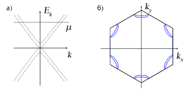
Figure 5: Fig. 5. (a) Energy structure of the graphene bilayer near Dirac points and (b) formation of the multisheet Fermi contour at weak doping.

Analysis of the conditions for the occurrence of Kohn-Luttinger superconductivity in the graphene bilayer is carried out in accordance with the general scheme described in Section 2. We consider the situation in which, as a result of doping, the chemical potential of the bilayer is in the two upper energy bands $E_{1\textbf{k}}$ and $E_{2\textbf{k}}$ as shown in Fig. 5a. In this case, the initial and final momenta of electrons in the Cooper channel also belong to the upper two bands; for this reason, indices $i$ and $j$ in the Kohn-Luttinger diagrams for a bilayer (see Fig. 1) acquire the values 1 or 2. Writing the analytical expressions for the diagrams, we obtain the analytic expression for the effective interaction of electrons in the Cooper channel of the graphene bilayer in Fig. 1, which can subsequently be used for analyzing the homogeneous part of the Bethe-Saltpeter equation. When solving eigenvalue problem (20), integration is carried out with the allowance for the multisheet nature of isoenergetic contours (Fig. 5b).

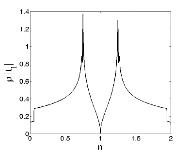
Figure 6: Fig. 6. Dependence of the electron density of states for the graphene bilayer per unit cell of one layer on the electron concentration for the set of parameters $t_{2}=0,\,\gamma_{1}=0.12|t_{1}|,\,\gamma_{3}=0.1|t_{1}|$.

Let us now consider the dependences of effective coupling constant $\lambda$ on carrier concentration $n$ for various types of symmetry of the superconducting order parameter in the graphene bilayer. It should be noted that in numerical calculations for the graphene bilayer for $\gamma_{1}=\gamma_{3}=\gamma_{4}=0$ and $G_{1}=G_{3}=G_{4}=0$, we get a limiting transition to the results obtained in Section 2 for a graphene monolayer. Figure 7 shows the $\lambda(n)$ dependences determined for the bilayer with the set of parameters $t_{2}=0,\,U=2|t_{1}|,\,\gamma_{1}=0.12|t_{1}|,\,\gamma_{3}=0.1|t_{1}|,\,\gamma_{4}=0$, and $V=G_{1}=G_{3}=G_{4}=0.5|t_{1}|$. The values of the intralayer and interlayer hopping integrals used here are close to the values determined in [61, 62] for graphite. The electron density of states for the graphene bilayer for the given set of parameters is shown in Fig. 6. To demonstrate the effect of the interlayer Coulomb interaction, we chose the maximal possible values of intensity $G_{1}$, $G_{3}$, and $G_{4}$ for which the weak-coupling approximation is still applicable. Comparison with Fig. 2b shows that the allowance for the interlayer interactions does not change the domains of superconductivity with the $f-$ and $d+id$-wave symmetry types; however, it leads to a significant increase in the absolute values of the effective coupling constant and, hence, to an increase in the superconducting transition temperature.

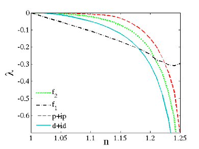
Figure 7: Fig. 7. Dependence of $\lambda$ on carrier concentration $n$ in the graphene bilayer for the set of parameters $t_{2}=0,\,U=2,\,\gamma_{1}=0.12,\,\gamma_{3}=0.1,\,V=0.5,\,G_{1}=G_{3}=G_{4}=0.5$ (all parameters are given in the units of $|t_{1}|$).

4 CONCLUSIONS

We have analyzed the conditions for the emergence of superconducting Kohn-Luttinger pairing in systems with a linear dispersion relation using as an example an idealized graphene monolayer and bilayer, disregarding the Van der Waals potential of the substrate and impurities. The electronic structure of graphene is described using the tight binding method in the Shubin-Vonsovsky model taking into account not only the Coulomb repulsion of electrons on the same carbon atom, but also the intersite Coulomb interaction. It is shown that the inclusion of the Kohn-Luttinger renormalizations up to the second order of perturbation theory inclusively and the allowance for the intersite Coulomb interaction determine to a considerable extent the competition between the superconducting phases with the $f-$ and $d+id$-wave types of the order parameter symmetry. They also lead to an increase in the absolute values of the effective interaction and, hence, to higher superconducting transition temperatures for the idealized graphene monolayer.

The results obtained for the graphene monolayer are generalized to the case of an idealized graphene bilayer consisting of two monolayers interacting via Coulomb repulsion between the layers. It is shown that the analysis of the idealized bilayer system of graphene leads to a considerably higher value of the superconducting transition temperature in the context of the Kohn-Luttinger mechanism.

References

- [1] Yu. E. Lozovik, S. P. Merkulova, and A. A. Sokolik, Phys. Usp. 51, 727 (2008).
- [2] A. H. Castro Neto, F. Guinea, N. M. R. Peres, K. S. Novoselov, and A. K. Geim, Rev. Mod. Phys. 81, 109 (2009).
- [3] V. N. Kotov, B. Uchoa, V. M. Pereira, F. Guinea, and A. H. Castro Neto, Rev. Mod. Phys. 84, 1067 (2012).
- [4] P. R. Wallace, Phys. Rev. 71, 622 (1947).
- [5] K. S. Novoselov, A. K. Geim, S. V. Morozov, D. Jiang, M. I. Katsnelson, I. V. Grigorieva, S. V. Dubonos, and A. A. Firsov, Nature (London) 438, 197 (2005).
- [6] Y.-W. Tan, Y. Zhang, K. Bolotin, Y. Zhao, S. Adam, E. H. Hwang, S. Das Sarma, H. L. Stormer, and P. Kim, Phys. Rev. Lett. 99, 246803 (2007).
- [7] S. V. Morozov, K. S. Novoselov, M. I. Katsnelson, F. Schedin, D. C. Elias, J. A. Jaszczak, and A. K. Geim, Phys. Rev. Lett. 100, 016602 (2008).
- [8] K. I. Bolotin, K. J. Sikes, Z. Jiang, M. Klima, G. Fudenberg, J. Hone, P. Kim, and H. L. Stormer, Solid State Commun. 146, 351 (2008).
- [9] N. Garcia, P. Esquinazi, J. Barzola-Quiquia, B. Ming, and D. Spoddig, Phys. Rev. B 78, 035413 (2008).
- [10] A. K. Geim, M. I. Katsnelson, and K. S. Novoselov, Nature Phys. 2, 620 (2006).
- [11] A. F. Young and P. Kim, Nature Phys. 5, 222 (2009).
- [12] M. I. Katsnelson, Eur. Phys. J. B 51, 157 (2006).
- [13] T. M. Rusin and W. Zawadzki, Phys. Rev. B 80, 045416 (2009).
- [14] P. R. Nair, P. Blake, A. N. Grigorenko, K. S. Novoselov, T. J. Booth, T. Stauber, N. M. R. Peres, and A. K. Geim, Science 320, 1308 (2008).
- [15] W. A. Muoz, L. Covaci, and F. M. Peeters, Phys. Rev. B 86, 184505 (2012).
- [16] H. B. Heersche, P. Jarillo-Herrero, J. B. Oostinga, L. M. K. Vandersypen, and A. F. Morpurgo, Nature (London) 446, 56 (2007).
- [17] A. Shailos, W. Nativel, A. Kasumov, C. Collet, M. Ferrier, S. Gueron, R. Deblock, and H. Bouchiat, Europhys. Lett. 79, 57008 (2007).
- [18] X. Du, I. Skachko, and E. Y. Andrei, Phys. Rev. B 77, 184507 (2008).
- [19] C. Ojeda-Aristizabal, M. Ferrier, S. Guéron, and H. Bouchiat, Phys. Rev. B 79, 165436 (2009).
- [20] A. Kanda, T. Sato, H. Goto, H. Tomori, S. Takana, Y. Ootuka, and K. Tsukagoshi, Physica C 470, 1477 (2010).
- [21] H. Tomori, A. Kanda, H. Goto, S. Takana, Y. Ootuka, and K. Tsukagoshi, Physica C 470, 1492 (2010).
- [22] N. M. R. Peres, F. Guinea, and A. H. Castro Neto, Phys. Rev. B 72, 174406 (2005).
- [23] E. C. Marino and L. H. C. M. Nunes, Nucl. Phys. B 741, 404 (2006).
- [24] J. González, F. Guinea, and M. A. H. Vozmediano, Phys. Rev. B 63, 134421 (2001).
- [25] B. Uchoa and A. H. Castro Neto, Phys. Rev. Lett. 98, 146801 (2007).
- [26] A. M. Black-Schaffer and S. Doniach, Phys. Rev. B 75, 134512 (2007).
- [27] C. Honerkamp, Phys. Rev. Lett. 100, 146404 (2008).
- [28] J. González, Phys. Rev. B 78, 205431 (2008).
- [29] R. S. Markiewicz, J. Phys. Chem. Solids 58, 1179 (1997).
- [30] W. Kohn and J. M. Luttinger, Phys. Rev. Lett. 15, 524 (1965).
- [31] D. Fay and A. Layzer, Phys. Rev. Lett. 20, 187 (1968).
- [32] M. Yu. Kagan and A. V. Chubukov, JETP Lett. 47, 614 (1988).
- [33] M. A. Baranov, A. V. Chubukov, and M. Yu. Kagan, Int. J. Mod. Phys. B 6, 2471 (1992).
- [34] R. Nandkishore, L. S. Levitov, and A. V. Chubukov, Nature Phys. 8, 158 (2012).
- [35] B. Valenzuela and M. A. H. Vozmediano, New J. Phys. 10, 113009 (2008).
- [36] J. L. McChesney, A. Bostwick, T. Ohta, T. Seyller, K. Horn, J. González, and E. Rotenberg, Phys. Rev. Lett. 104, 136803 (2010).
- [37] M. L. Kiesel, C. Platt, W. Hanke, D. A. Abanin, and R. Thomale, Phys. Rev. B 86, 020507(R) (2012).
- [38] T. O. Wehling, E. Şaşıoğlu, C. Friedrich, A. I. Lichtenstein, M. I. Katsnelson, and S. Blugel, Phys. Rev. Lett. 106, 236805 (2011).
- [39] J. González, Phys. Rev. B 88, 125434 (2013).
- [40] E. H. Hwang and S. Das Sarma, Phys. Rev. Lett. 101, 156802 (2012).
- [41] A. B. Migdal, Sov. Phys. JETP 7, 996 (1958).
- [42] W. Kohn, Phys. Rev. Lett. 2, 393 (1959).
- [43] J. Friedel, Adv. Phys. 3, 446 (1954); Nuovo Cimento Suppl. 2, 287 (1958).
- [44] M. Yu. Kagan, Phys. Lett. A 152, 303 (1991).
- [45] M. Yu. Kagan and V. V. Val’kov, 140, 179 (2011); Low Temp. Phys. 37, 84 (2011); A Lifetime in Magnetism and Superconductivity: A Tribute to Professor David Schoenberg, Cambridge Scientific Publishers, Cambridge, 2011.
- [46] A. A. Levin, Solid State Quantum Chemistry, McGraw-Hill, New York, 1977.
- [47] E. Perfetto, M. Cini, S. Ugenti, P. Castrucci, M. Scarselli, M. De Crescenzi, F. Rosei, and M. A. El Khakani, Phys. Rev. B 76, 233408 (2007).
- [48] S. Shubin and S. Vonsowsky, Proc. Roy. Soc. A 145, 159 (1934); Phys. Zs. UdSSR 7, 292 (1935); 10, 348 (1936).
- [49] L. P. Gor’kov and T. K. Melik-Barkhudarov, Sov. Phys. JETP 13, 1018 (1961).
- [50] D. J. Scalapino, E. Loh, Jr., and J. E. Hirsch, Phys. Rev. B 34, 8190 (1986); 35, 6694 (1987).
- [51] R. Hlubina, Phys. Rev. B 59, 9600 (1999).
- [52] S. Raghu, S. A. Kivelson, and D. J. Scalapino, Phys. Rev. B 81, 224505 (2010).
- [53] A. S. Alexandrov and V. V. Kabanov, Phys. Rev. Lett. 106, 136403 (2011).
- [54] M. Yu. Kagan, V. V. Val kov, V. A. Mitskan, and M. M. Korovushkin, JETP Lett. 97, 226 (2013); JETP 117, 728 (2013).
- [55] L. D. Landau and E. M. Lifshitz, Course of Theoretical Physics, Vol. 3: Quantum Mechanics: Non-Relativistic Theory, Butterworth-Heinemann, Oxford, 1991.
- [56] I. E. Dzyaloshinskii and V. M. Yakovenko, Sov. Phys. JETP 67, 844 (1988); I. E. Dzyaloshinskii, I. M. Krichever, and J. Chronek, Sov. Phys. JETP 67, 1492 (1988).
- [57] A. T. Zheleznyak, V. M. Yakovenko, and I. E. Dzyaloshinskii, Phys. Rev. B 55, 3200 (1997).
- [58] M. Yu. Kagan, V. V. Val’kov, V. A. Mitskan, and M. M. Korovushkin, Solid State Commun. 188, 61 (2014).
- [59] E. McCann and V. I. Fal’ko, Phys. Rev. Lett. 96, 086805 (2006).
- [60] E. McCann and M. Koshino, Rep. Prog. Phys. 76, 056503 (2013).
- [61] M. S. Dresselhaus and G. Dresselhaus, Adv. Phys. 51, 1 (2002).
- [62] N. B. Brandt, S. M. Chudinov, and Y. G. Ponomarev, in Modern Problems in Condensed Matter Sciences, edited by V. M. Agranovich and A. A. Maradudin, North-Holland, Amsterdam, Vol 20.1, 1988.