Comparison of hydrodynamic model of graphene with recent experiment on measuring the Casimir interaction

Abstract

We obtain the reflection coefficients from a graphene sheet deposited on a material substrate under a condition that graphene is described by the hydrodynamic model. Using these coefficients, the gradient of the Casimir force in the configuration of recent experiment is calculated in the framework of the Lifshitz theory. It is shown that the hydrodynamic model is excluded by the measurement data at the 99% confidence level over a wide range of separations. From the fact that the same data are in a very good agreement with theoretical predictions of the Dirac model of graphene, the low-energy character of the Casimir interaction is confirmed.

I Introduction

Graphene is a two-dimensional sheet of carbon atoms which attracts much experimental and theoretical attention due to unique physical properties and great promise for various applications.1 The most often used approach describing the electric and optical properties of graphene is the Dirac model.2 It is applicable at low energies up to a few eV and assumes the linear dispersion relation for massless quasiparticles, which move with a Fermi velocity rather than with the speed of light.3 The Dirac model was applied by many authors to calculate the van der Waals, Casimir and Casimir-Polder interactions in layer systems including graphene (see, for instance, Refs.4 ; 5 ; 6 ; 7 ; 8 ). The most straightforward formalism for performing these calculations uses the polarization tensor in (2+1)-dimensional space-time.9 ; 10 ; 11 ; 12 ; 13 ; 14 Recently an equivalence of the formalisms exploiting the polarization tensor and the density-density correlation function has been proven.15 Furthermore, the formalism of the polarization tensor was applied16 ; 17 for comparison with the measurement data of recent experiment18 and demonstrated a very good agreement.

Another approach used in theoretical description of the properties of graphene is the hydrodynamic model.19 ; 20 This model considers graphene as an infinitesimally thin positively charged sheet, carrying a homogeneous fluid with some mass and negative charge densities. In the framework of this model, the dispersion relation for quasiparticles in graphene is quadratic with respect to the momentum. The hydrodynamic model was also considered and applied to calculate the van der Waals, Casimir and Casimir-Polder interactions in many papers.11 ; 12 ; 21 ; 22 ; 23 ; 23a ; 24 ; 25a ; 25 ; 25b It was found11 that in the interaction of graphene with either a Si or a Au plate the hydrodynamic model predicts larger magnitudes of the Casimir free energy than the Dirac model.

In this paper, we compare theoretical predictions of the hydrodynamic model with the experimental data of recent measurement18 of the gradient of the Casimir force between a Au-coated sphere and a graphene sheet deposited on a SiO₂ film covering a Si plate. For this purpose, we derive exact expressions for the reflection coefficients of the electromagnetic oscillations on a three-layer structure, where one layer is a two-dimensional sheet described by the hydrodynamic model, whereas two other layers are described by the frequency-dependent dielectric permittivities. Then, the Casimir force and its gradient are calculated by using the standard Lifshitz theory26 ; 27 in the proximity force approximation27 (PFA). We demonstrate that theoretical predictions of the hydrodynamic model are excluded by the measurement data at the 99% confidence level over a wide region of separations between the sphere and the graphene sheet. This allows to conclude that the hydrodynamic model of graphene does not describe such physical phenomena, as the van der Waals and Casimir forces.

The paper is organized as follows. In Sec. II we derive the reflection coefficients for a graphene-coated substrate under an assumption that graphene is described by the hydrodynamic model. Using these reflection coefficients, in Sec. III we calculate the gradient of the Casimir force in the experimental configuration of recent experiment18 and compare the theoretical results with the experimental data. Section IV contains our conclusions and discussion.

II Reflection coefficients in the hydrodynamic model

We consider the amplitude reflection coefficients $R^{(g,s)}$ from a graphene sheet deposited on a thick plate (semispace) made of an ordinary material. Let us denote the reflection coefficient from a freestanding graphene sheet by $r^{(g)}$ and from a semispace in vacuum by $r^{(s)}$. Then, for the transverse magnetic (TM) and transverse electric (TE) polarizations of the electromagnetic field one obtains 16

$$R_{\rm TM,TE}^{(g,s)}=\frac{r_{\rm TM,TE}^{(g)}+r_{\rm TM,TE}^{(s)}(1\mp 2r_{\rm TM,TE}^{(g)})}{1-r_{\rm TM,TE}^{(g)}r_{\rm TM,TE}^{(s)}}.$$ (1)

Here, the signs minus and plus should be chosen for the TM and TE polarizations, respectively.

In the framework of the hydrodynamic model, the reflection coefficients $r^{(g)}$ for a graphene sheet in vacuum calculated at the Matsubara frequencies along the imaginary frequency axis take the form 11 ; 12 ; 21 ; 22 ; 23 ; 24 ; 25 ; 27

$$r_{\rm TM}^{(g)}\equiv r_{\rm TM}^{(g)}(i\xi_{l},k_{\bot})=\frac{c^{2}q_{l}K}{c^{2}q_{l}K+\xi_{l}^{2}},$$

$$r_{\rm TE}^{(g)}\equiv r_{\rm TE}^{(g)}(i\xi_{l},k_{\bot})=-\frac{K}{K+q_{l}}.$$ (2)

Here, the Matsubara frequencies are $\xi_{l}=2\pi k_{B}Tl/\hbar$, $k_{B}$ is the Boltzmann constant, $T$ is the temperature, $l=0,\,1,\,2,\,\ldots\,$, $q_{l}^{2}=k_{\bot}^{2}+\xi_{l}^{2}/c^{2}$, $k=|\mbox{\boldmath$k$}_{\bot}|$, and $\mbox{\boldmath$k$}_{\bot}$ is the projection of the wave vector on the plane of graphene. The quantity $K$ is the the single parameter characterizing graphene in the framework of the hydrodynamic model. It has the meaning of the wave number of a graphene sheet and is determined by the parameters of the hexagonal structure of graphite (one $\pi$-electron per atom, resulting in two $\pi$-electrons per hexagonal cell). Calculation leads to 19 ; 20 ; 21

$$K=2\pi\frac{ne^{2}}{mc^{2}}=6.75\times 10^{5}\,\mbox{m}^{-1},$$ (3)

where $e$ and $m$ are the charge and mass of $\pi$-electrons and $n=4/(3\sqrt{3}l^{2})$ with $l=1.421\,$Å being the side length of the hexagon in a crystal lattice. The wave number in Eq. (3) corresponds to the frequency $\omega_{K}=cK=2.02\times 10^{14}\,$rad/s.

The reflection coefficients $r^{(s)}$ from the boundary plane of a semispace described by the dielectric permittivity $\varepsilon_{1l}\equiv\varepsilon_{1}(i\xi_{l})$ are the well known Fresnel coefficients

$$r_{\rm TM}^{(s)}\equiv r_{\rm TM}^{(s)}(i\xi_{l},k_{\bot})=\frac{\varepsilon_{1l}q_{l}-k_{1l}}{\varepsilon_{1l}q_{l}+k_{1l}},$$

$$r_{\rm TE}^{(s)}\equiv r_{\rm TE}^{(s)}(i\xi_{l},k_{\bot})=\frac{q_{l}-k_{1l}}{q_{l}+k_{1l}},$$ (4)

where

$$k_{1l}^{2}\equiv k_{1}^{2}(i\xi_{l},k_{\bot})=k_{\bot}^{2}+\varepsilon_{1l}\frac{\xi_{l}^{2}}{c^{2}}.$$ (5)

Substituting Eqs. (2) and (4) in Eq. (1), we find the reflection coefficients from a graphene sheet deposited on a semispace made of ordinary material

$$R_{\rm TM}^{(g,s)}\equiv R_{\rm TM}^{(g,s)}(i\xi_{l},k_{\bot})=\frac{\varepsilon_{1l}q_{l}\xi_{l}^{2}-k_{1l}\xi_{l}^{2}+2c^{2}q_{l}Kk_{1l}}{\varepsilon_{1l}q_{l}\xi_{l}^{2}+k_{1l}\xi_{l}^{2}+2c^{2}q_{l}Kk_{1l}},$$

$$R_{\rm TE}^{(g,s)}\equiv R_{\rm TE}^{(g,s)}(i\xi_{l},k_{\bot})=\frac{q_{l}-k_{1l}-2K}{q_{l}+k_{1l}+2K}.$$ (6)

For computational purposes, we express the reflection coefficients (6) in terms of the dimensionless variables

$$y=2aq_{l},\qquad\zeta_{l}=\frac{2a\xi_{l}}{c},$$ (7)

where $a$ is a parameter having the dimension of length (in the next section $a$ has the meaning of separation distance between a graphene-coated substrate and a sphere). Then one arrives at

$$R_{\rm TM}^{(g,s)}\equiv R_{\rm TM}^{(g,s)}(i\zeta_{l},y)=\frac{\varepsilon_{1l}y\zeta_{l}^{2}-\tilde{k}_{1l}\zeta_{l}^{2}+2\tilde{K}y\tilde{k}_{1l}}{\varepsilon_{1l}y\zeta_{l}^{2}+\tilde{k}_{1l}\zeta_{l}^{2}+2\tilde{K}y\tilde{k}_{1l}},$$

$$R_{\rm TE}^{(g,s)}\equiv R_{\rm TE}^{(g,s)}(i\zeta_{l},y)=\frac{y-\tilde{k}_{1l}-2\tilde{K}}{y+\tilde{k}_{1l}+2\tilde{K}},$$ (8)

where

$$\tilde{k}_{1l}^{2}=4a^{2}k_{1l}^{2}=y^{2}+(\varepsilon_{1l}-1)\zeta_{l}^{2},\qquad\tilde{K}=2aK.$$ (9)

III Comparison of the hydrodynamic model with the measurement data

In the first experiment on the Casimir effect in systems including graphene, the gradient of the Casimir force was measured between a Au-coated hollow glass sphere of radius $R=54.1\,\mu$m and a graphene sheet deposited on a SiO₂ film covering a Si plate.18 The thickness of a SiO₂ film was $D=300\,$nm. The thickness of a Si plate ($500\,\mu$m) was large enough to consider it as a Si semispace when calculating the Casimir force. In a similar way, the Au coating on a sphere resulted in the same Casimir force as an all-Au sphere. Measurements were performed by means of dynamic atomic microscope operated in the frequency-shift technique.28 ; 29 ; 30 ; 31 ; 32 The force-distance relations were obtained with different applied voltages (20 repetitions) and with applied compensating voltages (22 repetitions) over the separation region from 224 to 500 nm for two different graphene samples. All the mean gradients of the Casimir force were found to be in a very good mutual agreement in the limits of the experimental errors.18 As an example, in Fig. 1(a,b) typical mean gradients of the Casimir force (the first sample, the measurement results obtained with applied compensating voltage) are shown as crosses at different separations $a$ between the sphere and the plate. The vertical arms of the crosses indicate twice the total error $\Delta F^{\prime}=0.64\,\mu$N/m in measurements of the gradient of the Casimir force, and the horizontal arms are twice the error $\Delta a=0.4\,$nm in measurement of absolute separations. These errors were found at the 67% confidence level, i.e., the true values of the force gradients and separations with a probability of 67% belong to the intervals $[F^{\prime}(a)-\Delta F^{\prime},F^{\prime}(a)+\Delta F^{\prime}]$ and $[a-\Delta a,a+\Delta a]$, respectively.

Using the Lifshitz theory and the PFA, the gradient of the Casimir force between a Au sphere and a graphene sheet deposited on a SiO₂ film covering a Si plate (semispace) is given by

$$F^{\prime}(a)=\frac{k_{B}TR}{4a^{3}}\sum_{l=0}^{\infty}\!{\vphantom{\sum}}^{\prime}\int_{\zeta_{l}}^{\infty}\!\!\!y^{2}dy\left[\frac{r_{\rm TM}^{(\rm Au)}(i\zeta_{l},y)R_{\rm TM}^{(g,f,s)}(i\zeta_{l},y)}{e^{y}-r_{\rm TM}^{(\rm Au)}(i\zeta_{l},y)R_{\rm TM}^{(g,f,s)}(i\zeta_{l},y)}\right.$$

$$~{}~{}~{}~{}\left.+\frac{r_{\rm TE}^{(\rm Au)}(i\zeta_{l},y)R_{\rm TE}^{(g,f,s)}(i\zeta_{l},y)}{e^{y}-r_{\rm TE}^{(\rm Au)}(i\zeta_{l},y)R_{\rm TE}^{(g,f,s)}(i\zeta_{l},y)}\right],$$ (10)

Here, $T=300\,$K is the temperature at the laboratory, the prime on the summation sign multiplies by 1/2 the term with $l=0$, and the dimensionless variables $y$ and $\zeta_{l}$ are introduced in Eq. (7). The reflection coefficients from a Au semispace (which replaces a sphere in the PFA) are given by Eq. (4). In terms of dimensionless variables, they take the form

$$r_{\rm TM}^{(\rm Au)}(i\zeta_{l},y)=\frac{\varepsilon_{l}^{\,(\rm Au)}y-\tilde{k}_{l}^{(\rm Au)}}{\varepsilon_{l}^{\,(\rm Au)}y+\tilde{k}_{l}^{(\rm Au)}},$$

$$r_{\rm TE}^{(\rm Au)}(i\zeta_{l},y)=\frac{y-\tilde{k}_{l}^{(\rm Au)}}{y+\tilde{k}_{l}^{(\rm Au)}},$$ (11)

where, in accordance to Eq. (9),

$$\tilde{k}_{l}^{(\rm Au)}=[y^{2}+(\varepsilon_{l}^{\,(\rm Au)}-1)\zeta_{l}^{2}]^{1/2}.$$ (12)

The reflection coefficients from a graphene sheet deposited on a SiO₂ (fused silica) film covering a Si plate are expressed by the standard formulas of the Lifshitz theory between layered structures27 ; 33

$$R_{\rm TM,TE}^{(g,f,s)}(i\zeta_{l},y)=\frac{R_{\rm TM,TE}^{(g,s)}(i\zeta_{l},y)+r_{\rm TM,TE}^{(f,s)}(i\zeta_{l},y)e^{-2D\tilde{k}_{1l}/(2a)}}{1+R_{\rm TM,TE}^{(g,s)}(i\zeta_{l},y)r_{\rm TM,TE}^{(f,s)}(i\zeta_{l},y)e^{-2D\tilde{k}_{1l}/(2a)}}.$$ (13)

Here, the reflection coefficients $R_{\rm TM,TE}^{(g,s)}$ describe the reflection from a graphene sheet deposited on a SiO₂ semispace. If graphene is described by the hydrodynamic model, they are given by Eq. (8) with $\varepsilon_{1l}=\varepsilon^{({\rm SiO}_{2})}(ic\zeta_{l}/2a)$. The coefficients $r_{\rm TM,TE}^{(f,s)}$ describe the reflection on the boundary plane between the two semispaces made of SiO₂ and Si. They are the standard Fresnel reflection coefficients:

$$r_{\rm TM}^{(f,s)}(i\zeta_{l},y)=\frac{\varepsilon_{2l}\tilde{k}_{1l}-\varepsilon_{1l}\tilde{k}_{2l}}{\varepsilon_{2l}\tilde{k}_{1l}+\varepsilon_{1l}\tilde{k}_{2l}}$$

$$r_{\rm TE}^{(f,s)}(i\zeta_{l},y)=\frac{\tilde{k}_{1l}-\tilde{k}_{2l}}{\tilde{k}_{1l}+\tilde{k}_{2l}},$$ (14)

where $\varepsilon_{2l}\equiv\varepsilon^{\,(\rm Si)}(ic\zeta_{l}/2a)$ and $\tilde{k}_{2l}$ is defined similar to Eq. (9) with a replacement of $\varepsilon_{1l}$ with $\varepsilon_{2l}$.

The quantity $\varepsilon_{l}^{(\rm Au)}\equiv\varepsilon^{(\rm Au)}(ic\zeta_{l}/2a)$ entering Eq. (11) is found 27 ; 28 using the Kramers-Kronig relation from the measured optical data 34 for ${\rm Im}\,\varepsilon^{(\rm Au)}$ extrapolated to zero frequency either by the Drude model with the plasma frequency $\omega_{p}=9.0\,$eV and relaxation parameter $\gamma=0.035\,$eV or by the nondissipative plasma model. Note that the above values of the Drude parameters are in a very good agreement with the measured optical data.35 Contrary to the expectations, the most precise experiments on measuring the Casimir interaction between metallic surfaces 27 ; 28 ; 29 ; 30 ; 31 ; 36 ; 37 ; 38 ; 39 are in agreement with the theoretical predictions using the plasma model extrapolation of the optical data and exclude the theoretical results using the Drude model extrapolation. Deep physical reasons why the plasma model extrapolation of the optical data is in agreement with the most precise measurements and the Drude model extrapolation is excluded by them remain unknown. Here, we perform all computations using both extrapolations for Au. We find that for a sphere interacting with a graphene-coated substrate, where graphene is described by the hydrodynamic model, the difference arising from using different extrapolations is rather small. This allows to include it in the magnitude of the theoretical error like it was done in the case of metal-graphene interaction computed using the Dirac model of graphene.11 ; 16 ; 18

In order to calculate the reflection coefficients (13) one also needs the values of $\varepsilon^{(\rm Si)}$ and $\varepsilon^{({\rm SiO}_{2})}$ at the imaginary Matsubara frequencies. The B-doped Si plate used in the experiment 18 had a resistivity between 0.001 and 0.005 $\Omega$ cm. This corresponds 40 to a charge carrier density between $1.6\times 10^{19}$ and $7.8\times 10^{19}\,\mbox{cm}^{-3}$, i.e., well above the critical density at which the dielectric-to-metal phase transition accurs.41 Then one obtains for the plasma frequency 42 the values between $5\times 10^{14}$ and $11\times 10^{14}\,$rad/s and for the relaxation parameter 31 $\gamma\approx 1.1\times 10^{14}\,$rad/s. These Drude parameters were used to extrapolate the optical data 43 for ${\rm Im}\,\varepsilon^{(\rm Si)}$ to zero frequency by means of either the Drude or the plasma model. Finally, the dielectric permittivity of Si at the imaginary Matsubara frequencies was found by means of the Kramers-Kronig relation like this was done previously in the literature.44 Different types of extrapolation for a Si lead to only minor differences in the computed force gradients in the experimental configuration. This is also taken into account in the theoretical error. For the dielectric permittivity of SiO₂ an accurate analytic expression 45 has been used.

The theoretical force gradients using the hydrodynamic model of graphene were computed by Eqs. (8), (10), (11), (13), and (14). The computational results were corrected for the presence of surface roughness which contribution does not exceed 0.1% in this experiment.16 The computed gradients of the Casimir force are shown as blue bands in Fig. 1(a,b) over the entire measurement range. The uncertainty in the values of $\omega_{p}$ of Si and the differences between the predictions of the Drude and plasma model extrapolations of the optical data for Au and Si determine the theoretical error, which is taken into account in the width of the bands. As is seen in Fig. 1, the theoretical description of graphene using the hydrodynamic model is excluded by the data at the 67% confidence level over the entire measurement range from 224 to 500 nm. With increasing confidence level, the error bars of the mean force gradients and separation distances are also increasing. Thus, at the 95% confidence level the maximum increase of the error bars is by a factor of two.27 ; 46 Note that if the errors are determined at the 95% or 99% confidence levels the true values of the force gradients and separations belong to the wider intervals $[F^{\prime}(a)-\Delta F^{\prime},F^{\prime}(a)+\Delta F^{\prime}]$ and $[a-\Delta a,a+\Delta a]$ with probabilities of 95% and 99%, respectively. Taking this into account, it can be seen that over the range of separations from 224 to 450 nm theoretical predictions of the hydrodynamic model are excluded by the data at a higher, 95% confidence level. If we further increase the confidence level up to 99%, it is easily seen that theoretical predictions of the hydrodynamic model are still excluded, but this time over a more narrow separation range up to 360 nm.

It is interesting also to compare the theoretical predictions of the hydrodynamic model with theoretical predictions of the Dirac model over a wider separation region from 220 nm to $1\,\mu$m. In Fig. 2 the gradients of the Casimir force in the configuration of an experiment18 computed in this paper using the hydrodynamic model (the dashed line) and using the Dirac model16 ; 17 (the solid line) are shown as functions of separation. As is seen in Fig. 2, the predictions of the hydrodynamic model remain to be larger than the experimentally consistent predictions of the Dirac model. The physical reason why the hydrodynamic model is not suitable for theoretical description of the Casimir force in layered systems including graphene may be in the linear dispersion relation inherent to graphene at low energies. This property makes a big difference between graphene and all types of ordinary dielectrics and metals.

IV Conclusions and discussion

In this paper, we have compared the measurement results for the gradient of the Casimir force between a Au-coated sphere and a graphene-coated substrate 18 with theoretical predictions of the hydrodynamic model of graphene used by many authors in previous literature. For this purpose, the reflection coefficients from the three-layer structure, where the first layer is graphene described by the hydrodynamic model and two other layers are described by the frequency-dependent dielectric permittivities, have been obtained. It was shown that the hydrodynamic model of graphene is excluded by the measurement data over the entire measurement range from 224 to 500 nm at the 67% confidence level. Over a narrower separation region from 224 to 360 nm an exclusion of the hydrodynamic model by the data at even higher 99% confidence level is demonstrated.

The same experimental data 18 was recently shown 16 to be in a very good agreement with theoretical predictions using the Dirac model of graphene. Keeping in mind that the Dirac model is applicable at energies below a few eV, the results of this paper provide additional arguments in favor of the low-energy character of the Casimir interaction. In future it would be interesting to apply the hydrodynamic model for theoretical description of the reflectivity of graphene at higher energies, outside the applicability region of the Dirac model, and perform a comparison with respective experimental results.

         

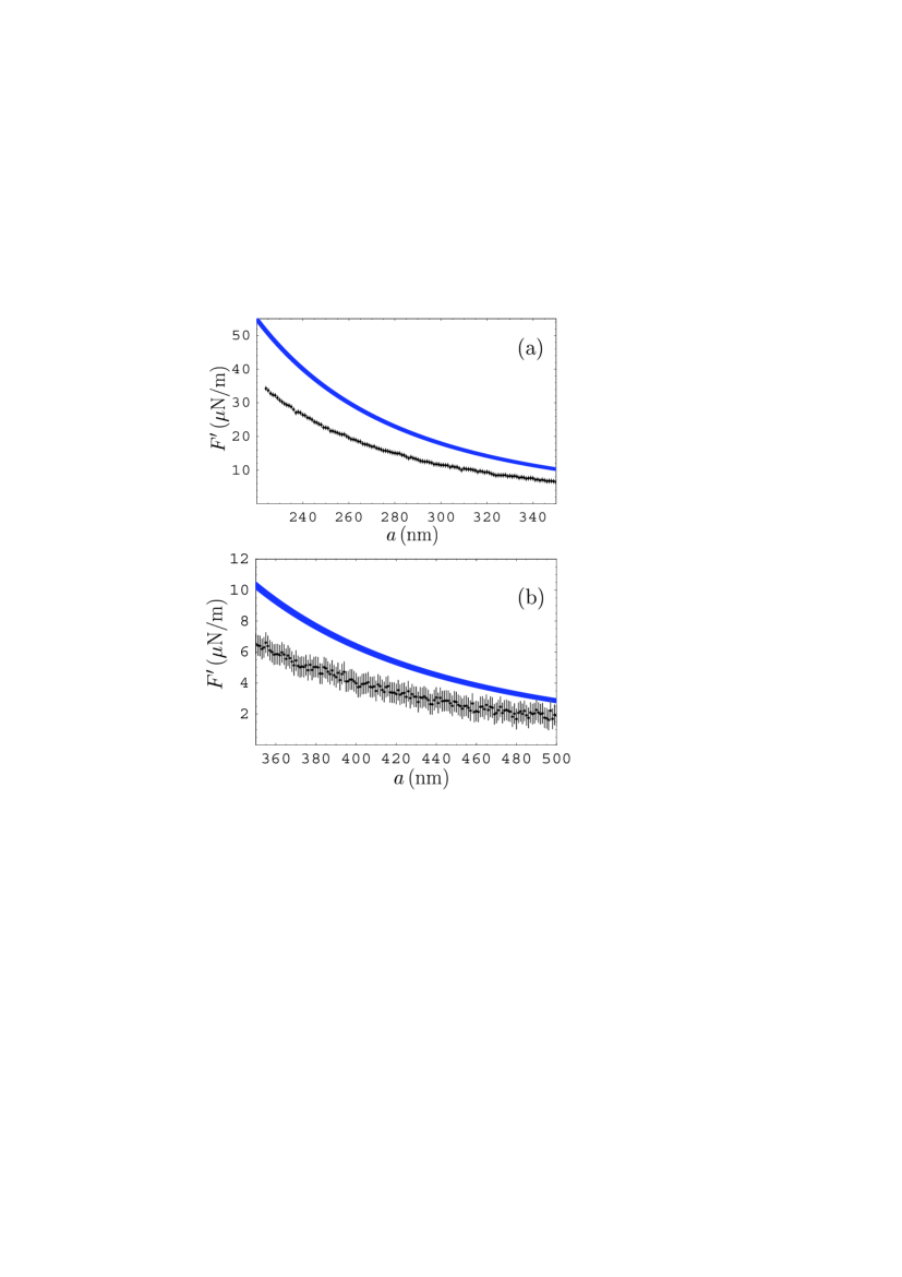
Figure 1: (Color online) The experimental data for the gradient of the Casimir force between a Au-coated sphere and a graphene sheet deposited on a SiO₂ film covering a Si plate (the first sample) are shown as crosses plotted at a 67% confidence level over different separation regions (a) from 224 to 350 nm and (b) from 350 to 500 nm. The respective theoretical predictions of the hydrodynamic model of graphene are indicated as the blue bands.

         

Figure 2: The gradients of the Casimir force between a Au-coated sphere and a graphene sheet deposited on a SiO₂ film covering a Si plate are computed using the hydrodynamic model (the dashed line) and the Dirac model (the solid line) as functions of separation.

References

- (1) M. I. Katsnelson, Graphene: Carbon in Two Dimensions (Cambridge University Press, Cambridge, 2012).
- (2) A. K. Geim and K. S. Novoselov, Nature Mater. 6, 183 (2007).
- (3) A. H. Castro Neto, F. Guinea, N. M. R. Peres, K. S. Novoselov, and A. K. Geim, Rev. Mod. Phys. 81, 109 (2009).
- (4) G. Gómez-Santos, Phys. Rev. B 80, 245424 (2009).
- (5) D. Drosdoff and L. M. Woods, Phys. Rev. B 82, 155459 (2010).
- (6) D. Drosdoff and L. M. Woods, Phys. Rev. A 84, 062501 (2011).
- (7) Bo E. Sernelius, Europhys. Lett. 95, 57003 (2011).
- (8) D. Drosdoff, A. D. Phan, L. M. Woods, I. V. Bondarev, and J. F. Dobson, Eur. Phys. J. B 85, 365 (2012).
- (9) M. Bordag, I. V. Fialkovsky, D. M. Gitman, and D. V. Vassilevich, Phys. Rev. B 80, 245406 (2009).
- (10) I. V. Fialkovsky, V. N. Marachevsky, and D. V. Vassilevich, Phys. Rev. B 84, 035446 (2011).
- (11) M. Bordag, G. L. Klimchitskaya, and V. M. Mostepanenko, Phys. Rev. B 86, 165429 (2012).
- (12) Yu. V. Churkin, A. B. Fedortsov, G. L. Klimchitskaya, and V. A. Yurova, Phys. Rev. B 82, 165433 (2010).
- (13) M. Chaichian, G. L. Klimchitskaya, V. M. Mostepanenko, and A. Tureanu, Phys. Rev. A 86, 012515 (2012).
- (14) G. L. Klimchitskaya and V. M. Mostepanenko, Phys. Rev. B 87, 075439 (2013).
- (15) G. L. Klimchitskaya, V. M. Mostepanenko, and Bo E. Sernelius, Phys Rev. B 89, 125407 (2014).
- (16) G. L. Klimchitskaya, U. Mohideen, and V. M. Mostepanenko, Phys. Rev. B 89, 115419 (2014).
- (17) G. L. Klimchitskaya and V. M. Mostepanenko, Phys. Rev. A 89, 052512 (2014).
- (18) A. A. Banishev, H. Wen, J. Xu, R. K. Kawakami, G. L. Klimchitskaya, V. M. Mostepanenko, and U. Mohideen, Phys. Rev. B 87, 205433 (2013).
- (19) G. Barton, J. Phys. A 37, 1011 (2004).
- (20) G. Barton, J. Phys. A 38, 2997 (2005).
- (21) M. Bordag, J. Phys. A: Math. Gen. 39, 6173 (2006).
- (22) M. Bordag, B. Geyer, G. L. Klimchitskaya, and V. M. Mostepanenko, Phys. Rev. B 74, 205431 (2006).
- (23) E. V. Blagov, G. L. Klimchitskaya, and V. M. Mostepanenko, Phys. Rev. B 75, 235413 (2007).
- (24) M. Bordag and N. Khusnutdinov, Phys. Rev. D 77, 085026 (2008).
- (25) T. E. Judd, R. G. Scott, A. M. Martin, B. Kaczmarek, and T. M. Fromhold, New. J. Phys. 13, 083020 (2011).
- (26) N. R. Khusnutdinov, Phys. Rev. B 83, 115454 (2011).
- (27) B. Arora, H. Kaur, and B. K. Sahoo, J. Phys. B 47, 155002 (2014).
- (28) M. Bordag, Phys. Rev. D 89, 125015 (2014).
- (29) E. M. Lifshitz and L. P. Pitaevskii, Statistical Physics, Pt.II (Pergamon Press, Oxford, 1980).
- (30) M. Bordag, G. L. Klimchitskaya, U. Mohideen, and V. M. Mostepanenko, Advances in the Casimir Effect (Oxford University Press, Oxford, 2009).
- (31) G. L. Klimchitskaya, U. Mohideen, and V. M. Mostepanenko, Rev. Mod. Phys. 81, 1827 (2009).
- (32) C.-C. Chang, A. A. Banishev, R. Castillo-Garza, G. L. Klimchitskaya, V. M. Mostepanenko, and U. Mohideen, Phys. Rev. B 85, 165443 (2012).
- (33) A. A. Banishev, C.-C. Chang, G. L. Klimchitskaya, V. M. Mostepanenko, and U. Mohideen, Phys. Rev. B 85, 195422 (2012).
- (34) A. A. Banishev, G. L. Klimchitskaya, V. M. Mostepanenko, and U. Mohideen, Phys. Rev. Lett. 110, 137401 (2013).
- (35) A. A. Banishev, G. L. Klimchitskaya, V. M. Mostepanenko, and U. Mohideen, Phys. Rev. B 88, 155410 (2013).
- (36) M. S. Tomaš, Phys. Rev. A 66, 052103 (2002).
- (37) Handbook of Optical Constants of Solids, ed. E. D. Palik (Academic, New York, 1985).
- (38) G. Bimonte, Phys. Rev. A 83, 042109 (2011).
- (39) R. S. Decca, E. Fischbach, G. L. Klimchitskaya, D. E. Krause, D. López, and V. M. Mostepanenko, Phys. Rev. D 68, 116003 (2003).
- (40) R. S. Decca, D. López, E. Fischbach, G. L. Klimchitskaya, D. E. Krause, and V. M. Mostepanenko, Ann. Phys. (N.Y.) 318, 37 (2005).
- (41) R. S. Decca, D. López, E. Fischbach, G. L. Klimchitskaya, D. E. Krause, and V. M. Mostepanenko, Phys. Rev. D 75, 077101 (2007).
- (42) R. S. Decca, D. López, E. Fischbach, G. L. Klimchitskaya, D. E. Krause, and V. M. Mostepanenko, Eur. Phys. J. C 51, 963 (2007).
- (43) Quick Reference Manual for Silicon Integrated Circuit Technology, eds. W. E. Beadle, J. C. C. Tsai, and R. D. Plummer (Wiley, New York, 1985).
- (44) P. Dai, Y. Zhang, and M. P. Sarachik, Phys. Rev. Lett. 66, 1914 (1991).
- (45) Semiconductors: Physics of Group IV Elements and III-V Compounds, ed. K.-H. Hellwege (Springer, Berlin, 1982).
- (46) Handbook of Optical Constants of Solids, vol II, ed. E. D. Palik (Academic, New York, 1991).
- (47) F. Chen, U. Mohideen, G. L. Klimchitskaya, and V. M. Mostepanenko, Phys. Rev. A 72, 020101(R) (2005); 74, 022103 (2006).
- (48) L. Bergström, Adv. Colloid Interface Sci. 70, 125 (1997).
- (49) S. G. Rabinovich, Measurement Errors and Uncertainties: Theory and Practice (Springer, New York, 2000).