Evaluating accuracy of community detection using the relative normalized mutual information

Abstract

The Normalized Mutual Information (NMI) has been widely used to evaluate the accuracy of community detection algorithms. However in this article we show that the NMI is seriously affected by systematic errors due to finite size of networks, and may give a wrong estimate of performance of algorithms in some cases. We give a simple theory to the finite-size effect of NMI and test our theory numerically. Then we propose a new metric for the accuracy of community detection, namely the relative Normalized Mutual Information (rNMI), which considers statistical significance of the NMI by comparing it with the expected NMI of random partitions. Our numerical experiments show that the rNMI overcomes the finite-size effect of the NMI.

Detection of community structures, which asks to group nodes in a network into groups, is a key problem in network science, computer science, sociology and biology. Many algorithms have been proposed for this problem, see ref. Fortunato (2010) for a review. However on a given network, different algorithms usually give different results. Thus evaluating performance of these algorithms and finding the best ones are of great importance.

Usually the evaluations are performed on benchmark networks each of which has a reference partition. These benchmarks include networks generated by generative models, like Stochastic Block Model Holland et al. (1983) and LFR model Lancichinetti et al. (2008), with a planted partition as the reference partition; and some real-world networks, like the famous Karate Club network Zachary (1977) and the Political Blog network Adamic and Glance (2005), with a partition annotated by domain experts as the reference partition. The accuracy of a community detection algorithm is usually represented using similarity between the reference partition and partition found by the algorithm — the larger similarity, the better performance the algorithm has on the benchmark.

Without losing generality, in what follows we call the reference partition $A$ and the detected partition $B$, and our task is to study the measure of similarity between partition $A$ and partition $B$.

When the number of groups are identical, $q_{A}=q_{B}=q$, the similarity can be easily defined by the overlap, which is the number of identical group labels in $A$ and $B$ maximized over all possible permutations:

$$O(A,B)=\max_{\pi}\left(\frac{1}{n}\sum_{i=1}^{n}\delta_{A_{i},\pi(B_{i})}-\frac{1}{q}\right),$$ (1)

where $n$ is number of nodes, $\delta$ is the Kronecker delta function and $\pi$ ranges over all permutations of $q$ groups.

However we can see that the overlap is non-zero even if partition $B$ is a random partition: there are roughly $\frac{n}{q}$ identical labels in two partitions if labels are distributed randomly and uniformly. One way to refine it is to normalize the overlap to scale from $0$ to $1$ Decelle et al. (2011); Krzakala et al. (2013):

$${{\mathcal{O}}(A,B)}=\max_{\pi}\left(\frac{1}{n}\sum_{i=1}^{n}\delta_{A_{i},\pi(B_{i})}-\frac{1}{q}\right)\left/\left(1-\frac{1}{q}\right)\right.\,.$$ (2)

However despite its simplicity, using overlap as the similarity has two problems: first, when number of groups $q$ is large, maximizing overlap over $q!$ permutations is difficult; second, when number of partitions, $q_{A}$ and $q_{B}$, are not identical, the overlap is ill-defined.

Another well-accepted measure of similarity is the Normalized Mutual Information (NMI) Danon et al. (2005); Ana and Jain (2003), which is well-defined even when $q_{A}\neq q_{B}$. Many studies use NMI to evaluate their algorithms or to compare different algorithms Lancichinetti and Fortunato (2009); Fortunato (2010). To define NMI we need to approximate the marginal probability of a randomly selected node being in group $a$ and $b$ by $P_{A}(a)=\frac{n_{a}}{n}$ and $P_{B}(b)=\frac{n_{b}}{n}$, where $n_{a}$ and $n_{b}$ denote group size of $A$ and $B$.

We know that the spirit of Mutual Information is to compute the dependence of these two distributions, by computing Kullback-Leibler (KL) distance between joint distribution $P_{AB}(a,b)$ and the product of two marginal distributions $P_{A}(a)P_{B}(b)$:

$$I_{AB}(P_{A},P_{B})=\sum_{a=1}^{q_{a}}\sum_{b=1}^{q_{b}}P_{AB}(a,b)\log\frac{P_{AB}(a,b)}{P_{A}(a)P_{B}(b)}.$$ (3)

Due to the property of KL distance, this quantity is non-negative. $I_{AB}(P_{A},P_{B})=0$ implies that $P_{A}$ and $P_{B}$ are independent, that detected partition has nothing to do with the ground-true partition. And if $I_{AB}(P_{A},P_{B})$ is much larger than zero, the detected partition and the ground true partition are similar. In practice the joint distribution can also be approximated by frequencies

$$P_{AB}(a,b)=\frac{n_{ab}}{n},$$

where $n_{ab}$ is number of nodes that both in group $a$ of partition $A$ and in group $b$ of partition $B$. Eq.(3) can be written as

$$I(P_{A},P_{B})=H(P_{A})+H(P_{B})-H(P_{AB}),$$ (4)

where

$$H(P_{A})=-\sum_{a}P_{A}(a)\log P_{A}(a)$$

is the Shannon entropy of distribution $P_{A}$, and $H(P_{AB})$ is the entropy of the joint distribution $P_{AB}$. Note that using conditional distribution $P_{A|B}(a|b)=P_{AB}(a,b)/P_{B}(b)$, one can rewrite Eq.(3) as

$$I(P_{A},P_{B})=H(P_{A})-H(P_{A|B}),$$ (5)

which has a interpretation that amount of information (surprise) gained on distribution $P_{A}$ after known $B$. If this information gain is $0$, it means knowledge of $B$ does not give any information about $A$, then two partitions has nothing to do with each other. Obviously the larger $I_{AB}(P_{A},P_{B})$, the more similar two partitions are. However this is still not a ideal metric for evaluating community detection algorithms since it is not normalized. As proposed in Danon et al. (2005), one way to normalize it is to choose normalization as $H(P_{A})+H(P_{B})$, and the Normalized Mutual Information is written as

$${\rm NMI}(P_{A},P_{B})=\frac{2I(P_{A},P_{B})}{H(P_{A})+H(P_{B})}.$$ (6)

Since $H(P_{AB})\leq H(P_{A})+H(P_{B})$, ${\rm NMI}(P_{A},P_{B})$ is bounded below by $0$. Also note that $H(P_{AB})=H(P_{A})=H(P_{B})$ when $A$ and $B$ are identical, which means in this case ${\rm NMI}(P_{A},P_{B})=1$.

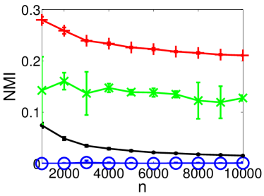
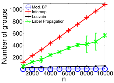
After NMI was introduced as a metric for comparing community detection algorithm, it becomes very popular in evaluating community detection algorithms. However in some cases we find that this metric gives un-consistent results. One example is shown in Fig. 1 left where we compare NMI between partitions obtained by four algorithms and the planted partition in the stochastic block model with parameter $\epsilon=1$. These four algorithms are Label Propagation Raghavan et al. (2007), Infomap Rosvall and Bergstrom (2008), Louvain method Blondel et al. (2008) and Modularity Belief Propagation Zhang and Moore (2014) respectively. The principle of the algorithms are different: Label Propagation algorithm maintains a group label for each node by iteratively adopting the label that most of its neighbors have; Infomap method compresses a description of information flow on the network; Louvain method maximizes modularity by aggregation; and Modularity Belief Propagation detects a statistically significant community structures using the landscape analysis in spin glass theory of statistical physics.

The stochastic block model (SBM) is also called the planted partition model. It has a planted, or ground-true, partition with $q$ groups of nodes, each node $i$ has a group label $t^{*}_{i}\in\{1,\ldots,q\}$. Edges in the network are generated independently according to a $q\times q$ matrix $p$, by connecting each pair of nodes $\left\langle ij\right\rangle$ with probability $p_{t^{*}_{i},t^{*}_{j}}$. Here we consider the commonly studied case where the $q$ groups have equal size and where $p$ has only two distinct entries, $p_{rs}=p_{\rm in}/n$ if $r=s$ and $p_{\rm out}/n$ if $r\neq s$. We use $\epsilon=p_{\rm out}/p_{\rm in}$ to denote the ratio between these two entries, the larger $\epsilon$ the weaker the community structure is. With $\epsilon=0$ the network is essentially composed of two connected components, while with $\epsilon=1$, as in Fig. 1 left, the network is deep in the un-detectable phase Decelle et al. (2011), and are essentially random graphs. In the later case though in each network there is a planted partition, the partition is not detectable in the sense that no algorithm could be able to find it or even find a partition that is correlated with it. This un-detectability of the planted partition in SBM has been proved for $q=2$ groups in Mossel12 .

However from Fig. 1 we can see that only Modularity BP gives zero NMI on all networks that is consistent with the un-detectability we described above, while other three algorithms give positive NMI, and Infomap gives a quite large NMI on all networks. Then the question arises: does it mean Infomap could do a theoretically-impossible job of finding the planted configuration in the un-detectable phase of SBM? We think it is not the case, but the problem comes from NMI, the measure for how much one finds about the planted configuration.

In Fig. 1 right we plot the number of groups found by different algorithms, then we can see that only Modularity BP gives one group while other algorithms report increasing number of groups when system size increases. Thus from this result we can guess that the large NMI found in Fig. 1 may come from a large number of group.

Figure 1: (Color online) Normalized Mutual Information (left) and number of groups (right) given by four algorithms on networks generated by Stochastic Block Model with $\epsilon=\frac{p_{\rm out}}{p_{\rm in}}=1$ (see text for the description of parameters of SBM), which is deep in the undetectable phase of SBM with different system sizes. These algorithms are (from top to bottom in left panel) Infomap Rosvall and Bergstrom (2008), Label Propagation Raghavan et al. (2007), Louvain method Blondel et al. (2008) and Modularity Belief Propagation Zhang and Moore (2014) . These networks are essentially random graphs, though in each network there is a planted partition, we expect no algorithm can obtain any information about it. Each point in the figure is averaged over $10$ realizations.

Recall that in computing NMI of two partitions, we use $\frac{n_{a}}{n}$ to approximate $p_{a}$, which is fine with $n\to\infty$ but leads to a finite size effect with $n$ finite. Since NMI can be seen as a function of entropies (as in Eq. (6)), we can express the finite size effect of NMI as the finite size effect of entropy, which means that entropy with an infinite system size $H_{\infty}(\left\{p_{a}\right\})$ is different from entropy with a finite system size $\left\langle H_{n}(\left\{n_{a}\right\})\right\rangle$, where the expectation is taken over random instances. Actually this effect comes from the fluctuations of $n_{a}$ around its mean value $p_{a}n$ and the concavity of entropy, as Jensen’s inequality implies that

$$\left\langle H_{n}(\left\{n_{a}\right\})\right\rangle\leq H_{\infty}(\left\{p_{a}\right\})=H_{\infty}(\left\{\left\langle\frac{n_{a}}{n}\right\rangle\right\}).$$

More precisely, we have

$$\left\langle H_{n}(\left\{n_{a}\right\})\right\rangle =-\sum_{a=1}^{q}\left\langle\frac{n_{a}}{n}\log\frac{n_{a}}{n}\right\rangle$$

$$=-\sum_{a=1}^{q}\left\langle p_{a}\log p_{a}+\left.\frac{\partial(x\log x)}{\partial x}\right|_{x=p_{a}}(\frac{n_{a}}{n}-p_{a})+\frac{1}{2}\left.\frac{\partial^{2}(x\log x)}{\partial x^{2}}\right|_{x=p_{a}}(\frac{n_{a}}{n}-p_{a})^{2}\right\rangle.$$

Assuming further on the distribution that the random variable $n_{a}$ follows, for example the Bernoulli distribution as in Herzel et al. (1994), the mean entropy at finite-size systems can be estimated by inserting the first and second moment into last equation:

$$\left\langle H_{n}(\left\{n_{a}\right\})\right\rangle =-\sum_{a=1}^{q}\left(p_{a}\log p_{a}+\frac{1-p_{a}}{2n}\right)$$

$$=H_{\infty}(\left\{p_{a}\right\})-\frac{q-1}{2n}.$$ (7)

Obviously using Eq. (4) the finite size correction for mutual information is

$$\left\langle I_{\infty}(P_{A},P_{B})\right\rangle-I_{n}(P_{A},P_{B})=\frac{q_{a}+q_{b}-q_{a}q_{b}-1}{2n}.$$

In our system, if we treat number of nodes in a network as sample size, the difference between NMI estimated using (6) in our network and in the network with an infinite number of nodes is expressed as

$$\left\langle{\rm NMI}_{n}(P_{A},P_{B})\right\rangle-{\rm NMI}_{\infty}(P_{A},P_{B})=\frac{1}{2n}\frac{q_{a}q_{b}-q_{a}-q_{b}+1}{H(P_{A})+H(P_{B})}.$$ (8)

One thing we can infer from last equation is that in finite-size networks, even two random partitions $A$ and $B$ have a non-vanishing NMI, and its value is

$${\rm NMI}^{\rm{random}}_{n}(q_{A},q_{B})\approx\frac{1}{2n}\frac{q_{a}q_{b}-q_{a}-q_{b}+1}{H(P_{A})+H(P_{B})}.$$ (9)

Note that in the last equation we put $\approx$ instead of $=$ because ${\rm NMI}^{\rm{random}}_{n}(q_{A},q_{B})$ represents NMI of an instance instead of the ensemble average.

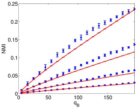
To test our theory on the finite-size correction, in Fig. 2 we compare NMI of two random partitions $A$ and $B$ with $q_{A}=10$ groups in partition $A$ and a varying number of groups in partition $B$. We can see that Eq. (9) gives a good estimate of NMI between two random partitions. From the figure we see that for the same $n$, the finite-size correction is smaller with fewer states. This is consistent with Eq. (9) whose right hand side is an increasing function of $q_{a}$ and $q_{b}$. Moreover we can see from the figure that for the same $q$, the finite-size correction is smaller with a larger system size, due to the $\frac{1}{n}$ dependence in Eq. (9). These two properties can also be used to understand the phenomenon we saw in Fig. 1 where NMI of Infomap and Label Propagation change slowly with system size, because number of groups given by these two algorithms increases in system size. We note that in Steuer et al. (2002) a similar finite-size effect for Mutual Information has been studied, though in a different context.

Figure 2: (Color online) Normalized Mutual Information between two random partitions $A$ and $B$. Partition $A$ always has $q_{A}=10$ groups, each of which has expected size $\frac{1}{q_{A}}$. While $B$ has a varying number of groups $q_{B}$, with expected group size $\frac{1}{q_{B}}$. In other words group labelling for each node is chosen independently according to $\frac{1}{q_{A}}$ for partition $A$ and $\frac{1}{q_{B}}$ for partition $B$. The lines are theoretical estimate (9) and points with error-bars are experimental data, with each point averaged over $10$ random instances. From top to bottom, system size are $n=1000$,$2000$,$4000$ and $8000$.

From above analysis, we see that as a metric for accuracy of community detection, NMI prefers a large number of partitions, which gives a systematic bias to evaluation results. One way to fix this bias is to consider statistical significance of the NMI, by comparing it to NMI of a null model. In this article we choose a random configuration $C$, which has the same group-size distribution as the detected partition, as a null model, and define the relative Normalized Mutual Information (rNMI) as

$${\rm rNMI}(A,B)={\rm NMI}(A,B)-\left\langle{\rm NMI}(A,C)\right\rangle,$$ (10)

where $\left\langle{\rm NMI}(A,C)\right\rangle$ is the expected NMI between the ground-true configuration $A$ and a random partition $C$, averaged over realizations of $C$.

So if partition $B$ has a large number of groups, though ${\rm NMI}(A,B)$ could be large, a random configuration having same distribution as $B$ also has a large number of groups and hence a large ${\rm NMI}(A,C)$ and finally results to a small ${\rm rNMI}(A,B)$.

Actually the idea of computing statistical significance by comparing score of a partition to expected score of a null model has been used everywhere in science. For example, the well-known metric for community structures, Modularity Newman and Girvan (2004), compares the number of internal edges of a partition to the expected number of internal edges in random graphs which act as a null model.

An easy way to compute $\left\langle{\rm NMI}(A,C)\right\rangle$ is to generate several random configurations, compute NMI for each random configuration then take the average. In practice we find that usually $10$ realizations of $C$ are already enough. If we really care about the computational speed, we can use expression

$$\left\langle{\rm NMI}(A,C)\right\rangle=\frac{1}{2n}\frac{q_{a}q_{b}-q_{a}-q_{b}+1}{H(P_{A})+H(P_{B})}.$$

However as explained in Eq. (Evaluating accuracy of community detection using the relative normalized mutual information), this expression is only a first-order approximation adopting the Bernoulli distribution, hence is obviously less accurate as the simulation value, as shown in Fig. 2.

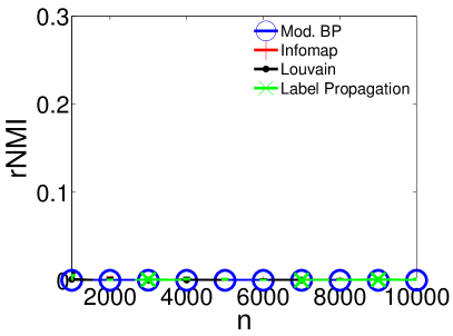
In Fig. 3 left we plot the rNMI given by the same four algorithms used in Fig. 1, where we can see that now all algorithms report zero rNMI, telling us correctly that no one has found useful information about the planted partition of SBM networks in the un-detectable phase.

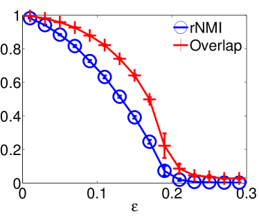
To test the accuracy of the proposed metric, in Fig. 3 right we compare the rNMI and overlap (Eq. (2)) between the planted partition and the one detected by Belief Propagation (BP) algorithm, for benchmark networks generated by stochastic block model. In this benchmark the detectability transition happens at $\epsilon^{*}=0.2$. It is known Decelle et al. (2011) that with $\epsilon<\epsilon^{*}$ the planted configuration is detectable, and BP algorithm is supposed to find a partition that is correlated with the planted configuration; with $\epsilon>\epsilon^{*}$ the planted configuration is un-detectable, which means that partition given by BP should be not correlated with the planted partition. In this case $q_{A}=q_{B}$, so overlap defined in (2) is a good metric and we can test whether rNMI gives the same information as overlap tells. In the figure we see that the value of rNMI and overlap are consistent: they are both high in detectable phase with $\epsilon<0.2$ and low in un-detectable phase with $\epsilon>0.2$. Note that the overlap is not perfectly zero in un-detectable phase, because in maximizing overlap over permutations the effect of noise has been induced. So in this sense our metric which reports perfectly zero values in un-detectable phase, is a better metric for similarity of two partitions in undetectable phase than overlap, even when $q_{A}=q_{B}$.

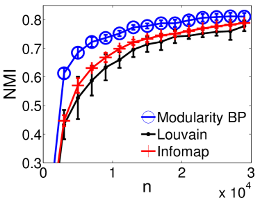
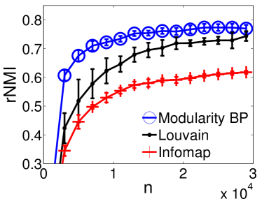
In Fig. 4 we compare NMI and rNMI for three algorithms, Louvain, Infomap and Modularity BP, on benchmark networks generated by the LFR model Lancichinetti et al. (2008) with different system sizes. the LFR model is also a planted model for generating benchmark networks with community structures. However compared with the SBM model, networks generated by the LFR model has a power-law degree distribution and group-size distribution. From left panel of Fig. 4 we can see that if we use the NMI as a metric for accuracy of these algorithms, we may conclude that Infomap works better than Louvain in whole set of benchmarks. However from Fig. 4 right we can see that Louvain actually works better than Infomap because it gives a larger rNMI than Infomap. Moreover the difference of rNMI between Louvain and Infomap are larger with system size increases. So Fig. 4 also tells us that using NMI may give a wrong estimate of performance of community detection algorithms.

Figure 3: (Color online) (Left) Relative Normalized Mutual Information given by the same four algorithms on the same set of networks used in Fig 1. Each point is averaged over $10$ realizations. (Right) Relative Normalized Mutual Information compared with overlap (2) in networks generated by stochastic block model with $10000$ nodes, $6$ groups, average degree $6$ and different $\epsilon=p_{\rm out}/p_{\rm in}$.

Figure 4: (Color online) Normalized Mutual Information (left) and Relative Normalized Mutual Information (right) for three algorithms, Infomap Rosvall and Bergstrom (2008), Louvain Blondel et al. (2008) and Modularity BP Zhang and Moore (2014) on LFR benchmarks Lancichinetti et al. (2008) with different system sizes. The parameters of networks are: average degree $c=8$, mixing parameter $\mu=0.45$, maximum degree is $50$, community sizes range from $200$ to $400$, exponent of degree distribution is $-2$. and exponent of community size distribution is $-1$.

As a conclusion, in this article we showed analytically and numerically that using normalized mutual information as a metric for accuracy of community detection algorithms has a systematic error when number of groups given by algorithms are much different. We proposed to fix this problem by using the relative normalize mutual information which considers the statistically significance of NMI by comparing the NMI of two partitions to the expected value of random partitions. We note that there are other ways to estimate finite-size effect of entropy, e.g. a Bayesian estimate proposed in Wolpert and DeDeo (2013). We put it in future work to refine $\left\langle{\rm NMI}(A,C)\right\rangle$ in expression of rNMI (10) using Bayesian approaches.

Implementation of rNMI and examples of using it can be found at code .