Jimm, a Fundamental Involution

A. Muhammed Uludağ, Hakan Ayral111 Galatasaray University, Department of Mathematics, Çırağan Cad. No. 36, 34357 Beşiktaş İstanbul, Turkey
Abstract

We study the involution of the real line induced by the outer automorphism of the extended modular group PGL(2,Z). This ‘modular’ involution is discontinuous at rationals but satisfies a surprising collection of functional equations. It preserves the set of real quadratic irrationalities mapping them in a highly non-obvious way to each other. It commutes with the Galois action on real quadratic irrationals.

More generally, it preserves set-wise the orbits of the modular group, thereby inducing an involution of the moduli space of real rank-two lattices. It induces a duality of Beatty partitions of the set of positive integers.

This involution conjugates (though not topologically) the Gauss’ continued fraction map to an intermittent dynamical system on the unit interval with an infinite invariant measure. The transfer operator (resp. the functional equation) naturally associated to this dynamical system is closely related to the Mayer transfer operator (resp. the Lewis’ functional equation).

We give a description of this involution as the boundary action of a certain automorphism of the infinite trivalent tree. We prove that its derivative exists and vanishes almost everywhere. It is conjectured that algebraic numbers of degree at least three are mapped to transcendental numbers under this involution.

Dedicated to Yılmaz Akyıldız, who shared our enthusiasm about jimm

1 Introduction

It is (it seems not very well-) known that the group $\mathrm{PGL}_{2}(\mathbf{Z})$ has an involutive outer automorphism, which was discovered by Dyer in the late 70’s [14]. It would be very strange if this automorphism had no manifestations in myriad contexts where $\mathrm{PGL}_{2}(\mathbf{Z})$ or its subgroups play a major role. Our aim in this paper is to elucidate one of these manifestations, which appears to have remained in obscurity until now. This may be because the conventional arithmetic, algebraic and geometric structures are not ‘respected’ by this involution (i.e. it sends parabolics to hyperbolics) which makes its study all the more appealing. Being thus exotic in several ways, we denote it - and some other involutions it gives rise to - by the letter222This is the fifth letter of the arabic alphabet in the hijâ’î order. Latex preamble commands for a latin-compatible typography of \RLj are given at the end of the paper. \RLj (read as: “jimm”), hoping that this notation will help to keep track of its manifestations.

Let $\widehat{\mathbf{R}}:=\mathbf{R}\cup\{\infty\}$. The manifestation in question of \RLj is a map \RLj𝐑:𝐑^𝐑^:subscript\RLj𝐑^𝐑^𝐑{\leavevmode\hbox{\raise 4.30554pt\hbox{\set@color\resizebox{}{}{\scalebox{0.8}[0.8]{{\leavevmode\hbox{\hskip 0.0pt\lower-0.19293pt\hbox{\set@color{\RL{j}}}}}}}}}}_{\mathbf{R}}:\widehat{\mathbf{R}}\rightarrow\widehat{\mathbf{R}}. Denoting the continued fractions in the usual way

$$[n_{0},n_{1},n_{2},\dots]=n_{0}+\cfrac{1}{n_{1}+\cfrac{1}{n_{2}+\cfrac{1}{\dots}}},$$

one has, for an irrational number $[n_{0},n_{1},n_{2},\dots]$ with $n_{0},n_{1},\dots\geq 2$,

\RLj𝐑([n0,n1,n2,])=[1n01,2,1n12,2,1n22,]subscript\RLj𝐑subscript𝑛0subscript𝑛1subscript𝑛2subscript1subscript𝑛012subscript1subscript𝑛122subscript1subscript𝑛22{\leavevmode\hbox{\raise 4.30554pt\hbox{\set@color\resizebox{}{}{\scalebox{0.8}[0.8]{{\leavevmode\hbox{\hskip 0.0pt\lower-0.19293pt\hbox{\set@color{\RL{j}}}}}}}}}}_{\mathbf{R}}([n_{0},n_{1},n_{2},\dots])=[1_{n_{0}-1},2,1_{n_{1}-2},2,1_{n_{2}-2},\dots] (1)

where $1_{k}$ is the sequence ${1,1,\dots,1}$ of length $k$. This formula remains valid for $n_{0},n_{1},\dots\geq 1$, if the emerging $1_{-1}$’s are eliminated in accordance with the rule $[\dots m,1_{-1},n,\dots]=[\dots m+n-1,\dots]$ and $1_{0}$ with the rule $[\dots m,1_{0},n,\dots]=[\dots m,n,\dots]$. See page 1 below for some examples.

It is possible to extend this definition of \RLj𝐑subscript\RLj𝐑{\leavevmode\hbox{\raise 4.30554pt\hbox{\set@color\resizebox{}{}{\scalebox{0.8}[0.8]{{\leavevmode\hbox{\hskip 0.0pt\lower-0.19293pt\hbox{\set@color{\RL{j}}}}}}}}}}_{\mathbf{R}} to all of $\widehat{\mathbf{R}}$. If we ignore rationals and the noble numbers (i.e. numbers in the $\mathrm{PGL}_{2}(\mathbf{Z})$-orbit of the golden section, $\Phi:=(1+\sqrt{5})/{2}$), then \RLj𝐑subscript\RLj𝐑{\leavevmode\hbox{\raise 4.30554pt\hbox{\set@color\resizebox{}{}{\scalebox{0.8}[0.8]{{\leavevmode\hbox{\hskip 0.0pt\lower-0.19293pt\hbox{\set@color{\RL{j}}}}}}}}}}_{\mathbf{R}} becomes an involution. It is well-defined and continuous at irrationals, but two-valued and discontinuous at rationals (Theorem 16). Although it is impossible to draw its graph, we will give (see page 4.3) a boxed-graph to indicate where the graph lies. One can choose one among the two values at rational arguments so that the function becomes upper semicontinuous. The amount of jump of \RLj𝐑subscript\RLj𝐑{\leavevmode\hbox{\raise 4.30554pt\hbox{\set@color\resizebox{}{}{\scalebox{0.8}[0.8]{{\leavevmode\hbox{\hskip 0.0pt\lower-0.19293pt\hbox{\set@color{\RL{j}}}}}}}}}}_{\mathbf{R}} at $q\in\mathbf{Q}$ provides a canonical (signed) measure of complexity of a rational number.

Guide for notation. In what follows,
\RLj denotes Dyers’ outer automorphism of $\mathrm{PGL}_{2}(\mathbf{Z})$,
\RLjsubscript\RLj{\leavevmode\hbox{\raise 4.30554pt\hbox{\set@color\resizebox{}{}{\scalebox{0.8}[0.8]{{\leavevmode\hbox{\hskip 0.0pt\lower-0.19293pt\hbox{\set@color{\RL{j}}}}}}}}}}_{\mathcal{F}} denotes the automorphism of the tree $|\mathcal{F}|$ induced by \RLj ,
\RLjsubscript\RLj{\leavevmode\hbox{\raise 4.30554pt\hbox{\set@color\resizebox{}{}{\scalebox{0.8}[0.8]{{\leavevmode\hbox{\hskip 0.0pt\lower-0.19293pt\hbox{\set@color{\RL{j}}}}}}}}}}_{\partial\mathcal{F}} denotes the homeomorphism of the boundary $\partial\mathcal{F}$ induced by \RLjsubscript\RLj{\leavevmode\hbox{\raise 4.30554pt\hbox{\set@color\resizebox{}{}{\scalebox{0.8}[0.8]{{\leavevmode\hbox{\hskip 0.0pt\lower-0.19293pt\hbox{\set@color{\RL{j}}}}}}}}}}_{\mathcal{F}},
\RLj𝐑subscript\RLj𝐑{\leavevmode\hbox{\raise 4.30554pt\hbox{\set@color\resizebox{}{}{\scalebox{0.8}[0.8]{{\leavevmode\hbox{\hskip 0.0pt\lower-0.19293pt\hbox{\set@color{\RL{j}}}}}}}}}}_{\mathbf{R}} denotes the involution of $\mathbf{R}$ induced by \RLjsubscript\RLj{\leavevmode\hbox{\raise 4.30554pt\hbox{\set@color\resizebox{}{}{\scalebox{0.8}[0.8]{{\leavevmode\hbox{\hskip 0.0pt\lower-0.19293pt\hbox{\set@color{\RL{j}}}}}}}}}}_{\partial\mathcal{F}}, and
\RLj𝐐subscript\RLj𝐐{\leavevmode\hbox{\raise 4.30554pt\hbox{\set@color\resizebox{}{}{\scalebox{0.8}[0.8]{{\leavevmode\hbox{\hskip 0.0pt\lower-0.19293pt\hbox{\set@color{\RL{j}}}}}}}}}}_{\mathbf{Q}} denotes the involution of $\mathbf{Q}\setminus\{0,\infty\}$ induced by \RLjsubscript\RLj{\leavevmode\hbox{\raise 4.30554pt\hbox{\set@color\resizebox{}{}{\scalebox{0.8}[0.8]{{\leavevmode\hbox{\hskip 0.0pt\lower-0.19293pt\hbox{\set@color{\RL{j}}}}}}}}}}_{\mathcal{F}}.
However, we reserve the right to drop the subscript and simply write \RLj when we think that confusion won’t arise.

Functional equations

The involution \RLj𝐑subscript\RLj𝐑{\leavevmode\hbox{\raise 4.30554pt\hbox{\set@color\resizebox{}{}{\scalebox{0.8}[0.8]{{\leavevmode\hbox{\hskip 0.0pt\lower-0.19293pt\hbox{\set@color{\RL{j}}}}}}}}}}_{\mathbf{R}} shares the privileged status of the fundamental involutions generating the extended modular group $\mathrm{PGL}_{2}(\mathbf{Z})$,

$$K:x\rightarrow 1-x,\quad U:x\rightarrow 1/x,\quad V:x\rightarrow-x,$$

as it interacts in a very harmonious way with them. Indeed, if we ignore its values at rational points then \RLj𝐑subscript\RLj𝐑{\leavevmode\hbox{\raise 4.30554pt\hbox{\set@color\resizebox{}{}{\scalebox{0.8}[0.8]{{\leavevmode\hbox{\hskip 0.0pt\lower-0.19293pt\hbox{\set@color{\RL{j}}}}}}}}}}_{\mathbf{R}} satisfies the following set of functional equations:

(FE:0)\RLj(\RLj(x))=x(FE:0)\RLj\RLj𝑥𝑥\mbox{(FE:0)}\quad{\leavevmode\hbox{\raise 4.30554pt\hbox{\set@color\resizebox{}{}{\scalebox{0.8}[0.8]{{\leavevmode\hbox{\hskip 0.0pt\lower-0.19293pt\hbox{\set@color{\RL{j}}}}}}}}}}({\leavevmode\hbox{\raise 4.30554pt\hbox{\set@color\resizebox{}{}{\scalebox{0.8}[0.8]{{\leavevmode\hbox{\hskip 0.0pt\lower-0.19293pt\hbox{\set@color{\RL{j}}}}}}}}}}(x))=x (FE:I)\RLjU=U\RLj\RLj(1x)=1\RLj(x)iff(FE:I)\RLj𝑈𝑈\RLj\RLj1𝑥1\RLj𝑥\mbox{(FE:I)}\quad{\leavevmode\hbox{\raise 4.30554pt\hbox{\set@color\resizebox{}{}{\scalebox{0.8}[0.8]{{\leavevmode\hbox{\hskip 0.0pt\lower-0.19293pt\hbox{\set@color{\RL{j}}}}}}}}}}U=U{\leavevmode\hbox{\raise 4.30554pt\hbox{\set@color\resizebox{}{}{\scalebox{0.8}[0.8]{{\leavevmode\hbox{\hskip 0.0pt\lower-0.19293pt\hbox{\set@color{\RL{j}}}}}}}}}}\iff{\leavevmode\hbox{\raise 4.30554pt\hbox{\set@color\resizebox{}{}{\scalebox{0.8}[0.8]{{\leavevmode\hbox{\hskip 0.0pt\lower-0.19293pt\hbox{\set@color{\RL{j}}}}}}}}}}\bigl{(}\frac{1}{x}\bigr{)}=\frac{1}{{\leavevmode\hbox{\raise 4.30554pt\hbox{\set@color\resizebox{}{}{\scalebox{0.8}[0.8]{{\leavevmode\hbox{\hskip 0.0pt\lower-0.19293pt\hbox{\set@color{\RL{j}}}}}}}}}}(x)} (FE:II)\RLjV=UV\RLj\RLj(x)=1\RLj(x)iff(FE:II)\RLj𝑉𝑈𝑉\RLj\RLj𝑥1\RLj𝑥\mbox{(FE:II)}\quad{\leavevmode\hbox{\raise 4.30554pt\hbox{\set@color\resizebox{}{}{\scalebox{0.8}[0.8]{{\leavevmode\hbox{\hskip 0.0pt\lower-0.19293pt\hbox{\set@color{\RL{j}}}}}}}}}}V=UV{\leavevmode\hbox{\raise 4.30554pt\hbox{\set@color\resizebox{}{}{\scalebox{0.8}[0.8]{{\leavevmode\hbox{\hskip 0.0pt\lower-0.19293pt\hbox{\set@color{\RL{j}}}}}}}}}}\iff{\leavevmode\hbox{\raise 4.30554pt\hbox{\set@color\resizebox{}{}{\scalebox{0.8}[0.8]{{\leavevmode\hbox{\hskip 0.0pt\lower-0.19293pt\hbox{\set@color{\RL{j}}}}}}}}}}(-x)=-\frac{1}{{\leavevmode\hbox{\raise 4.30554pt\hbox{\set@color\resizebox{}{}{\scalebox{0.8}[0.8]{{\leavevmode\hbox{\hskip 0.0pt\lower-0.19293pt\hbox{\set@color{\RL{j}}}}}}}}}}(x)} (FE:III)\RLjK=K\RLj\RLj(1x)=1\RLj(x)iff(FE:III)\RLj𝐾𝐾\RLj\RLj1𝑥1\RLj𝑥\mbox{(FE:III)}\quad{\leavevmode\hbox{\raise 4.30554pt\hbox{\set@color\resizebox{}{}{\scalebox{0.8}[0.8]{{\leavevmode\hbox{\hskip 0.0pt\lower-0.19293pt\hbox{\set@color{\RL{j}}}}}}}}}}K=K{\leavevmode\hbox{\raise 4.30554pt\hbox{\set@color\resizebox{}{}{\scalebox{0.8}[0.8]{{\leavevmode\hbox{\hskip 0.0pt\lower-0.19293pt\hbox{\set@color{\RL{j}}}}}}}}}}\iff{\leavevmode\hbox{\raise 4.30554pt\hbox{\set@color\resizebox{}{}{\scalebox{0.8}[0.8]{{\leavevmode\hbox{\hskip 0.0pt\lower-0.19293pt\hbox{\set@color{\RL{j}}}}}}}}}}(1-x)=1-{\leavevmode\hbox{\raise 4.30554pt\hbox{\set@color\resizebox{}{}{\scalebox{0.8}[0.8]{{\leavevmode\hbox{\hskip 0.0pt\lower-0.19293pt\hbox{\set@color{\RL{j}}}}}}}}}}(x)

The following set of functional equations are derived from the above ones:

(FE:II)\RLjUV=V\RLj\RLj(1x)=\RLj(x)iff(FE:II)\RLj𝑈𝑉𝑉\RLj\RLj1𝑥\RLj𝑥\mbox{(FE:II${}^{\prime}$)}\quad{\leavevmode\hbox{\raise 4.30554pt\hbox{\set@color\resizebox{}{}{\scalebox{0.8}[0.8]{{\leavevmode\hbox{\hskip 0.0pt\lower-0.19293pt\hbox{\set@color{\RL{j}}}}}}}}}}UV=V{\leavevmode\hbox{\raise 4.30554pt\hbox{\set@color\resizebox{}{}{\scalebox{0.8}[0.8]{{\leavevmode\hbox{\hskip 0.0pt\lower-0.19293pt\hbox{\set@color{\RL{j}}}}}}}}}}\iff{\leavevmode\hbox{\raise 4.30554pt\hbox{\set@color\resizebox{}{}{\scalebox{0.8}[0.8]{{\leavevmode\hbox{\hskip 0.0pt\lower-0.19293pt\hbox{\set@color{\RL{j}}}}}}}}}}(-\frac{1}{x})=-{{\leavevmode\hbox{\raise 4.30554pt\hbox{\set@color\resizebox{}{}{\scalebox{0.8}[0.8]{{\leavevmode\hbox{\hskip 0.0pt\lower-0.19293pt\hbox{\set@color{\RL{j}}}}}}}}}}(x)} (FE:IV)\RLjKV=KUV\RLj\RLj(1+x)=1+1\RLj(x)iff(FE:IV)\RLj𝐾𝑉𝐾𝑈𝑉\RLj\RLj1𝑥11\RLj𝑥\mbox{(FE:IV)}\quad{\leavevmode\hbox{\raise 4.30554pt\hbox{\set@color\resizebox{}{}{\scalebox{0.8}[0.8]{{\leavevmode\hbox{\hskip 0.0pt\lower-0.19293pt\hbox{\set@color{\RL{j}}}}}}}}}}KV=KUV{\leavevmode\hbox{\raise 4.30554pt\hbox{\set@color\resizebox{}{}{\scalebox{0.8}[0.8]{{\leavevmode\hbox{\hskip 0.0pt\lower-0.19293pt\hbox{\set@color{\RL{j}}}}}}}}}}\iff{\leavevmode\hbox{\raise 4.30554pt\hbox{\set@color\resizebox{}{}{\scalebox{0.8}[0.8]{{\leavevmode\hbox{\hskip 0.0pt\lower-0.19293pt\hbox{\set@color{\RL{j}}}}}}}}}}(1+x)=1+\frac{1}{{\leavevmode\hbox{\raise 4.30554pt\hbox{\set@color\resizebox{}{}{\scalebox{0.8}[0.8]{{\leavevmode\hbox{\hskip 0.0pt\lower-0.19293pt\hbox{\set@color{\RL{j}}}}}}}}}}(x)} (FE:V)(\RLj𝐑M\RLj𝐑)(x)=(\RLjM)(x)MPGL2(𝐙)formulae-sequence(FE:V)subscript\RLj𝐑𝑀subscript\RLj𝐑𝑥\RLj𝑀𝑥for-all𝑀subscriptPGL2𝐙\mbox{(FE:V)}\quad({\leavevmode\hbox{\raise 4.30554pt\hbox{\set@color\resizebox{}{}{\scalebox{0.8}[0.8]{{\leavevmode\hbox{\hskip 0.0pt\lower-0.19293pt\hbox{\set@color{\RL{j}}}}}}}}}}_{\mathbf{R}}M{\leavevmode\hbox{\raise 4.30554pt\hbox{\set@color\resizebox{}{}{\scalebox{0.8}[0.8]{{\leavevmode\hbox{\hskip 0.0pt\lower-0.19293pt\hbox{\set@color{\RL{j}}}}}}}}}}_{\mathbf{R}})(x)=({\leavevmode\hbox{\raise 4.30554pt\hbox{\set@color\resizebox{}{}{\scalebox{0.8}[0.8]{{\leavevmode\hbox{\hskip 0.0pt\lower-0.19293pt\hbox{\set@color{\RL{j}}}}}}}}}}M)(x)\quad\forall M\in\mathrm{PGL}_{2}(\mathbf{Z}) (FE:VI)\RLj𝐑(Mx)=\RLjM\RLj𝐑(x)MPGL2(𝐙)formulae-sequence(FE:VI)subscript\RLj𝐑𝑀𝑥\RLj𝑀subscript\RLj𝐑𝑥for-all𝑀subscriptPGL2𝐙\mbox{(FE:VI)}\quad{\leavevmode\hbox{\raise 4.30554pt\hbox{\set@color\resizebox{}{}{\scalebox{0.8}[0.8]{{\leavevmode\hbox{\hskip 0.0pt\lower-0.19293pt\hbox{\set@color{\RL{j}}}}}}}}}}_{\mathbf{R}}(Mx)={\leavevmode\hbox{\raise 4.30554pt\hbox{\set@color\resizebox{}{}{\scalebox{0.8}[0.8]{{\leavevmode\hbox{\hskip 0.0pt\lower-0.19293pt\hbox{\set@color{\RL{j}}}}}}}}}}M{\leavevmode\hbox{\raise 4.30554pt\hbox{\set@color\resizebox{}{}{\scalebox{0.8}[0.8]{{\leavevmode\hbox{\hskip 0.0pt\lower-0.19293pt\hbox{\set@color{\RL{j}}}}}}}}}}_{\mathbf{R}}(x)\quad\forall M\in\mathrm{PGL}_{2}(\mathbf{Z})


Equations (FE:I) and (FE:III) states that \RLj is covariant with the operators $U$ and $K$, whereas equation (FE:II) is a kind of lax-covariance Since $U$, $V$ and $K$ generate the group $\mathrm{PGL}_{2}(\mathbf{Z})$, we may say that \RLj is lax-covariant with the $\mathrm{PGL}_{2}(\mathbf{Z})$-action on $\mathbf{R}$. Of course, if we consider \RLj as an operator then covariance is simply a relation of commutativity. Relation (FE:IV) is not independent from the rest as it can be easily deduced from (FE:II) and (FE:III). The final relation is the most general form of the functional equations and says that \RLj𝐑subscript\RLj𝐑{\leavevmode\hbox{\raise 4.30554pt\hbox{\set@color\resizebox{}{}{\scalebox{0.8}[0.8]{{\leavevmode\hbox{\hskip 0.0pt\lower-0.19293pt\hbox{\set@color{\RL{j}}}}}}}}}}_{\mathbf{R}} conjugates the Möbius transformation $M\in\mathrm{PGL}_{2}(\mathbf{Z})$ to the Möbius transformation \RLj(M)PGL2(𝐙)\RLj𝑀subscriptPGL2𝐙{\leavevmode\hbox{\raise 4.30554pt\hbox{\set@color\resizebox{}{}{\scalebox{0.8}[0.8]{{\leavevmode\hbox{\hskip 0.0pt\lower-0.19293pt\hbox{\set@color{\RL{j}}}}}}}}}}(M)\in\mathrm{PGL}_{2}(\mathbf{Z}). It is readily deduced from (FE:I-III) by using the involutivity of \RLj . As an instance of (FE:V), \RLj conjugates the translation $1+x$ to $1+1/x$ and the transformation $1/(1+x)$ to $x/(1+x)$. (FE:VI) is got from (FE:V) by setting x\RLj𝐑(x)𝑥subscript\RLj𝐑𝑥x\to{\leavevmode\hbox{\raise 4.30554pt\hbox{\set@color\resizebox{}{}{\scalebox{0.8}[0.8]{{\leavevmode\hbox{\hskip 0.0pt\lower-0.19293pt\hbox{\set@color{\RL{j}}}}}}}}}}_{\mathbf{R}}(x). It says that \RLj𝐑subscript\RLj𝐑{\leavevmode\hbox{\raise 4.30554pt\hbox{\set@color\resizebox{}{}{\scalebox{0.8}[0.8]{{\leavevmode\hbox{\hskip 0.0pt\lower-0.19293pt\hbox{\set@color{\RL{j}}}}}}}}}}_{\mathbf{R}} is a kind of modular function.

Before attempting to play with them, beware that these functional equations are not consistent on the set of rational numbers. The first thing to try are the noble numbers. They are sent to rationals under \RLj and \RLj is 2-to-1 on this set. On the other hand, there is a related involution \RLj𝐐subscript\RLj𝐐{\leavevmode\hbox{\raise 4.30554pt\hbox{\set@color\resizebox{}{}{\scalebox{0.8}[0.8]{{\leavevmode\hbox{\hskip 0.0pt\lower-0.19293pt\hbox{\set@color{\RL{j}}}}}}}}}}_{\mathbf{Q}} on the set of positive rationals satisfying some functional equations. It must be stressed that \RLj𝐐subscript\RLj𝐐{\leavevmode\hbox{\raise 4.30554pt\hbox{\set@color\resizebox{}{}{\scalebox{0.8}[0.8]{{\leavevmode\hbox{\hskip 0.0pt\lower-0.19293pt\hbox{\set@color{\RL{j}}}}}}}}}}_{\mathbf{Q}} is not the restriction of \RLj𝐑subscript\RLj𝐑{\leavevmode\hbox{\raise 4.30554pt\hbox{\set@color\resizebox{}{}{\scalebox{0.8}[0.8]{{\leavevmode\hbox{\hskip 0.0pt\lower-0.19293pt\hbox{\set@color{\RL{j}}}}}}}}}}_{\mathbf{R}} to ${\mathbf{Q}}$. See page 3.2.

The privileged status of \RLj is vindicated by the fact that it preserves the “real-multiplication locus”, i.e. the set of real quadratic irrationalities. It does so in a highly non-trivial manner, though it preserves setwise the $\mathrm{PGL}_{2}(\mathbf{Z})$-orbits of real quadratic irrationalities. More generally \RLj preserves setwise the $\mathrm{PGL}_{2}(\mathbf{Z})$-orbits on $\widehat{\mathbf{R}}$ thereby inducing an involution of the moduli space of real rank-2 lattices, $\widehat{\mathbf{R}}/\mathrm{PGL}_{2}(\mathbf{Z})$. Moduli of the lattices represented by the numbers $[\overline{1_{k},k+2}]$ are fixed under this involution. For a precise description of all fixed points, see Proposition 25.

One could use the functional equations (FE:I)-(FE:III) to directly define and study the involution \RLj𝐑subscript\RLj𝐑{\leavevmode\hbox{\raise 4.30554pt\hbox{\set@color\resizebox{}{}{\scalebox{0.8}[0.8]{{\leavevmode\hbox{\hskip 0.0pt\lower-0.19293pt\hbox{\set@color{\RL{j}}}}}}}}}}_{\mathbf{R}}. However, the elusive nature of \RLj𝐑subscript\RLj𝐑{\leavevmode\hbox{\raise 4.30554pt\hbox{\set@color\resizebox{}{}{\scalebox{0.8}[0.8]{{\leavevmode\hbox{\hskip 0.0pt\lower-0.19293pt\hbox{\set@color{\RL{j}}}}}}}}}}_{\mathbf{R}} is best understood by considering it as a homeomorphism of the boundary of the Farey tree, induced by an automorphism of the tree. This automorphism is the one which twists all but one vertex of the tree.

Finally, the following two-variable consequence of the functional equations is noteworthy:

1x+1y=11\RLj(x)+1\RLj(y)=1iff1𝑥1𝑦11\RLj𝑥1\RLj𝑦1\boxed{\frac{1}{x}+\frac{1}{y}=1\iff\frac{1}{{\leavevmode\hbox{\raise 4.30554pt\hbox{\set@color\resizebox{}{}{\scalebox{0.8}[0.8]{{\leavevmode\hbox{\hskip 0.0pt\lower-0.19293pt\hbox{\set@color{\RL{j}}}}}}}}}}(x)}+\frac{1}{{\leavevmode\hbox{\raise 4.30554pt\hbox{\set@color\resizebox{}{}{\scalebox{0.8}[0.8]{{\leavevmode\hbox{\hskip 0.0pt\lower-0.19293pt\hbox{\set@color{\RL{j}}}}}}}}}}(y)}=1}

Hence \RLj sends harmonic pairs of numbers to harmonic pairs. See page 3.3 for a complete set of two-variable functional equations.

Recall that, if the pair $(x,y)$ satisfies ${1}/{x}+{1}/{y}=1$, then the so-called Beatty sequences $(\lfloor nx\rfloor)_{n\geq 1}$, $(\lfloor ny\rfloor)_{n\geq 1}$ gives a partition of the set of positive integers (Rayleigh’s theorem). Therefore every Beatty partition of positive integers admits a \RLj -dual partition (n\RLj(x))n1subscript𝑛\RLj𝑥𝑛1(\lfloor n{\leavevmode\hbox{\raise 4.30554pt\hbox{\set@color\resizebox{}{}{\scalebox{0.8}[0.8]{{\leavevmode\hbox{\hskip 0.0pt\lower-0.19293pt\hbox{\set@color{\RL{j}}}}}}}}}}(x)\rfloor)_{n\geq 1}, (n\RLj(y))n1.subscript𝑛\RLj𝑦𝑛1(\lfloor n{\leavevmode\hbox{\raise 4.30554pt\hbox{\set@color\resizebox{}{}{\scalebox{0.8}[0.8]{{\leavevmode\hbox{\hskip 0.0pt\lower-0.19293pt\hbox{\set@color{\RL{j}}}}}}}}}}(y)\rfloor)_{n\geq 1}.

Some examples.

Here is a list of assorted values of \RLj . Recall that $\Phi$ denotes the golden section.

Φ=[1¯]\RLj(Φ)==\RLj(1/Φ),Φdelimited-[]¯1\RLjΦ\RLj1Φ\displaystyle\Phi=[\overline{1}]\implies{\leavevmode\hbox{\raise 4.30554pt\hbox{\set@color\resizebox{}{}{\scalebox{0.8}[0.8]{{\leavevmode\hbox{\hskip 0.0pt\lower-0.19293pt\hbox{\set@color{\RL{j}}}}}}}}}}(\Phi)=\infty={\leavevmode\hbox{\raise 4.30554pt\hbox{\set@color\resizebox{}{}{\scalebox{0.8}[0.8]{{\leavevmode\hbox{\hskip 0.0pt\lower-0.19293pt\hbox{\set@color{\RL{j}}}}}}}}}}\bigl{(}-{1}/{\Phi}\bigr{)}, (2)

where by $\overline{v}$ we denote the infinite sequence $v,v,v,\dots$, for any finite sequence $v$. From 2 by using (FE:II) we find

\RLj(Φ)=\RLj(1/Φ)=0.\RLjΦ\RLj1Φ0\displaystyle{\leavevmode\hbox{\raise 4.30554pt\hbox{\set@color\resizebox{}{}{\scalebox{0.8}[0.8]{{\leavevmode\hbox{\hskip 0.0pt\lower-0.19293pt\hbox{\set@color{\RL{j}}}}}}}}}}(-\Phi)={\leavevmode\hbox{\raise 4.30554pt\hbox{\set@color\resizebox{}{}{\scalebox{0.8}[0.8]{{\leavevmode\hbox{\hskip 0.0pt\lower-0.19293pt\hbox{\set@color{\RL{j}}}}}}}}}}\bigl{(}{1}/{\Phi}\bigr{)}=0. (3)

Repeated application of (FE:IV) gives

\RLj(n+Φ)=\RLj([n+1,1¯])=Fn+1/Fn\RLj𝑛Φ\RLj𝑛1¯1subscript𝐹𝑛1subscript𝐹𝑛\displaystyle{\leavevmode\hbox{\raise 4.30554pt\hbox{\set@color\resizebox{}{}{\scalebox{0.8}[0.8]{{\leavevmode\hbox{\hskip 0.0pt\lower-0.19293pt\hbox{\set@color{\RL{j}}}}}}}}}}(n+\Phi)={\leavevmode\hbox{\raise 4.30554pt\hbox{\set@color\resizebox{}{}{\scalebox{0.8}[0.8]{{\leavevmode\hbox{\hskip 0.0pt\lower-0.19293pt\hbox{\set@color{\RL{j}}}}}}}}}}([n+1,\overline{1}])={F_{n+1}}/{F_{n}} (4)

where $F_{n}$ denotes the $n$th Fibonacci number. One has

\RLj([1n,2,1¯])=[n+1,]=n+1\RLjsubscript1𝑛2¯1𝑛1𝑛1{\leavevmode\hbox{\raise 4.30554pt\hbox{\set@color\resizebox{}{}{\scalebox{0.8}[0.8]{{\leavevmode\hbox{\hskip 0.0pt\lower-0.19293pt\hbox{\set@color{\RL{j}}}}}}}}}}([1_{n},2,\overline{1}])=[n+1,\infty]=n+1

For the number $\sqrt{2}$ we have something that looks simple

2=[1,2¯]\RLj(2)=[2¯]=1+221¯2\RLj2delimited-[]¯212\sqrt{2}=[1,\overline{2}]\implies{\leavevmode\hbox{\raise 4.30554pt\hbox{\set@color\resizebox{}{}{\scalebox{0.8}[0.8]{{\leavevmode\hbox{\hskip 0.0pt\lower-0.19293pt\hbox{\set@color{\RL{j}}}}}}}}}}(\sqrt{2})=[\overline{2}]=1+\sqrt{2}

but this is not typical as the next example illustrates:

\RLj((3+52)/7)=\RLj([1,2,3,1,1,2,1,1,1¯])=[2,2,1,4,5¯]=3+2957\RLj3527\RLj1¯231121112¯214532957{\leavevmode\hbox{\raise 4.30554pt\hbox{\set@color\resizebox{}{}{\scalebox{0.8}[0.8]{{\leavevmode\hbox{\hskip 0.0pt\lower-0.19293pt\hbox{\set@color{\RL{j}}}}}}}}}}({(3+5\sqrt{2})}/{7})={\leavevmode\hbox{\raise 4.30554pt\hbox{\set@color\resizebox{}{}{\scalebox{0.8}[0.8]{{\leavevmode\hbox{\hskip 0.0pt\lower-0.19293pt\hbox{\set@color{\RL{j}}}}}}}}}}([1,\overline{2,3,1,1,2,1,1,1}])=[2,\overline{2,1,4,5}]=\frac{-3+2\sqrt{95}}{7}

In a similar vein, consider the examples

11=[3;3,6¯]\RLj(11)=[1,1,2,1,2,1,1¯]=15+90126,113¯36\RLj11delimited-[]¯11212111590126\sqrt{11}=[3;\overline{3,6}]\implies{\leavevmode\hbox{\raise 4.30554pt\hbox{\set@color\resizebox{}{}{\scalebox{0.8}[0.8]{{\leavevmode\hbox{\hskip 0.0pt\lower-0.19293pt\hbox{\set@color{\RL{j}}}}}}}}}}(\sqrt{11})=[\overline{1,1,2,1,2,1,1}]=\frac{15+\sqrt{901}}{26},
\RLj(11)=1/\RLj(11)=2615+901=1590126.\RLj111\RLj1126159011590126{\leavevmode\hbox{\raise 4.30554pt\hbox{\set@color\resizebox{}{}{\scalebox{0.8}[0.8]{{\leavevmode\hbox{\hskip 0.0pt\lower-0.19293pt\hbox{\set@color{\RL{j}}}}}}}}}}(-\sqrt{11})=-1/{\leavevmode\hbox{\raise 4.30554pt\hbox{\set@color\resizebox{}{}{\scalebox{0.8}[0.8]{{\leavevmode\hbox{\hskip 0.0pt\lower-0.19293pt\hbox{\set@color{\RL{j}}}}}}}}}}(\sqrt{11})=-\frac{26}{15+\sqrt{901}}=\frac{15-\sqrt{901}}{26}.

The last example hints at the following result

Theorem 1

The involution \RLj commutes with the conjugation of real quadratic irrationals; i.e. for every real quadratic irrational $\alpha$ one has \RLj(α)=\RLj(α).\RLjsuperscript𝛼\RLjsuperscript𝛼{\leavevmode\hbox{\raise 4.30554pt\hbox{\set@color\resizebox{}{}{\scalebox{0.8}[0.8]{{\leavevmode\hbox{\hskip 0.0pt\lower-0.19293pt\hbox{\set@color{\RL{j}}}}}}}}}}({\alpha}^{*})={{\leavevmode\hbox{\raise 4.30554pt\hbox{\set@color\resizebox{}{}{\scalebox{0.8}[0.8]{{\leavevmode\hbox{\hskip 0.0pt\lower-0.19293pt\hbox{\set@color{\RL{j}}}}}}}}}}(\alpha)^{*}}.

Proof. Every real quadratic irrational $\alpha$ is the fixed point of some $M\in\mathrm{PSL}_{2}(\mathbf{Z})$, the Galois conjugate $\alpha^{*}$ being the other root of the equation $Mx=x$. But then \RLj(Mα)=\RLj(M)\RLj(α)=\RLj(α)\RLj𝑀𝛼\RLj𝑀\RLj𝛼\RLj𝛼{\leavevmode\hbox{\raise 4.30554pt\hbox{\set@color\resizebox{}{}{\scalebox{0.8}[0.8]{{\leavevmode\hbox{\hskip 0.0pt\lower-0.19293pt\hbox{\set@color{\RL{j}}}}}}}}}}(M\alpha)={\leavevmode\hbox{\raise 4.30554pt\hbox{\set@color\resizebox{}{}{\scalebox{0.8}[0.8]{{\leavevmode\hbox{\hskip 0.0pt\lower-0.19293pt\hbox{\set@color{\RL{j}}}}}}}}}}(M){\leavevmode\hbox{\raise 4.30554pt\hbox{\set@color\resizebox{}{}{\scalebox{0.8}[0.8]{{\leavevmode\hbox{\hskip 0.0pt\lower-0.19293pt\hbox{\set@color{\RL{j}}}}}}}}}}(\alpha)={\leavevmode\hbox{\raise 4.30554pt\hbox{\set@color\resizebox{}{}{\scalebox{0.8}[0.8]{{\leavevmode\hbox{\hskip 0.0pt\lower-0.19293pt\hbox{\set@color{\RL{j}}}}}}}}}}(\alpha), i.e. \RLj(α)\RLj𝛼{\leavevmode\hbox{\raise 4.30554pt\hbox{\set@color\resizebox{}{}{\scalebox{0.8}[0.8]{{\leavevmode\hbox{\hskip 0.0pt\lower-0.19293pt\hbox{\set@color{\RL{j}}}}}}}}}}(\alpha) is a fixed point of the equation \RLj(M)\RLj𝑀{\leavevmode\hbox{\raise 4.30554pt\hbox{\set@color\resizebox{}{}{\scalebox{0.8}[0.8]{{\leavevmode\hbox{\hskip 0.0pt\lower-0.19293pt\hbox{\set@color{\RL{j}}}}}}}}}}(M), the other root being \RLj(α)\RLjsuperscript𝛼{\leavevmode\hbox{\raise 4.30554pt\hbox{\set@color\resizebox{}{}{\scalebox{0.8}[0.8]{{\leavevmode\hbox{\hskip 0.0pt\lower-0.19293pt\hbox{\set@color{\RL{j}}}}}}}}}}(\alpha)^{*}. Finally

Mα=αMα=α\RLj(α)=\RLj(Mα)=\RLj(M)\RLj(α),𝑀𝛼𝛼𝑀superscript𝛼superscript𝛼\RLjsuperscript𝛼\RLj𝑀superscript𝛼\RLj𝑀\RLjsuperscript𝛼M\alpha=\alpha\implies M\alpha^{*}=\alpha^{*}\implies{\leavevmode\hbox{\raise 4.30554pt\hbox{\set@color\resizebox{}{}{\scalebox{0.8}[0.8]{{\leavevmode\hbox{\hskip 0.0pt\lower-0.19293pt\hbox{\set@color{\RL{j}}}}}}}}}}(\alpha^{*})={\leavevmode\hbox{\raise 4.30554pt\hbox{\set@color\resizebox{}{}{\scalebox{0.8}[0.8]{{\leavevmode\hbox{\hskip 0.0pt\lower-0.19293pt\hbox{\set@color{\RL{j}}}}}}}}}}(M\alpha^{*})={\leavevmode\hbox{\raise 4.30554pt\hbox{\set@color\resizebox{}{}{\scalebox{0.8}[0.8]{{\leavevmode\hbox{\hskip 0.0pt\lower-0.19293pt\hbox{\set@color{\RL{j}}}}}}}}}}(M){\leavevmode\hbox{\raise 4.30554pt\hbox{\set@color\resizebox{}{}{\scalebox{0.8}[0.8]{{\leavevmode\hbox{\hskip 0.0pt\lower-0.19293pt\hbox{\set@color{\RL{j}}}}}}}}}}(\alpha^{*}),

so \RLj(α)\RLjsuperscript𝛼{\leavevmode\hbox{\raise 4.30554pt\hbox{\set@color\resizebox{}{}{\scalebox{0.8}[0.8]{{\leavevmode\hbox{\hskip 0.0pt\lower-0.19293pt\hbox{\set@color{\RL{j}}}}}}}}}}(\alpha^{*}) is also a fixed point of \RLj(M)\RLj𝑀{\leavevmode\hbox{\raise 4.30554pt\hbox{\set@color\resizebox{}{}{\scalebox{0.8}[0.8]{{\leavevmode\hbox{\hskip 0.0pt\lower-0.19293pt\hbox{\set@color{\RL{j}}}}}}}}}}(M), i.e. it must coincide with \RLj(α)\RLjsuperscript𝛼{\leavevmode\hbox{\raise 4.30554pt\hbox{\set@color\resizebox{}{}{\scalebox{0.8}[0.8]{{\leavevmode\hbox{\hskip 0.0pt\lower-0.19293pt\hbox{\set@color{\RL{j}}}}}}}}}}(\alpha)^{*}. $\Box$.

To finish, let us give the \RLj -transform of a non-quadratic algebraic number,

\RLj(32)=\RLj([1;3,1,5,1,1,4,1,1,8,1,14,1,10,2,1,4,12,2,3,2,1,3,4,1,])\displaystyle{\leavevmode\hbox{\raise 4.30554pt\hbox{\set@color\resizebox{}{}{\scalebox{0.8}[0.8]{{\leavevmode\hbox{\hskip 0.0pt\lower-0.19293pt\hbox{\set@color{\RL{j}}}}}}}}}}(^{3}\!\sqrt{2})={\leavevmode\hbox{\raise 4.30554pt\hbox{\set@color\resizebox{}{}{\scalebox{0.8}[0.8]{{\leavevmode\hbox{\hskip 0.0pt\lower-0.19293pt\hbox{\set@color{\RL{j}}}}}}}}}}([1;3,1,5,1,1,4,1,1,8,1,14,1,10,2,1,4,12,2,3,2,1,3,4,1,\dots])
$\displaystyle=[2,1,3,1,1,1,4,1,1,4,1_{6},3,1_{12},3,1_{8},2,3,1,1,2,1_{10},2,2,1,2,3,1,2,1,1,3,\dots]$
$\displaystyle=2.784731558662723\dots$

and the transforms of two familiar transcendental numbers:

\RLj(π)=\RLj([3,7,15,1,292,1,1,1,2,1,3,])=[12,2,15,2,113,3,1290,5,3,]\RLj𝜋\RLj37151292111213subscript122subscript152subscript1133subscript129053\displaystyle{\leavevmode\hbox{\raise 4.30554pt\hbox{\set@color\resizebox{}{}{\scalebox{0.8}[0.8]{{\leavevmode\hbox{\hskip 0.0pt\lower-0.19293pt\hbox{\set@color{\RL{j}}}}}}}}}}(\pi)={\leavevmode\hbox{\raise 4.30554pt\hbox{\set@color\resizebox{}{}{\scalebox{0.8}[0.8]{{\leavevmode\hbox{\hskip 0.0pt\lower-0.19293pt\hbox{\set@color{\RL{j}}}}}}}}}}([3,7,15,1,292,1,1,1,2,1,3,\dots])=[1_{2},2,1_{5},2,1_{13},3,1_{290},5,3,\dots]
$\displaystyle=1.7237707925480276079699326494931025145558144289232\dots$
\RLj(e)=\RLj([2,1,2,1,1,4,1,1,6,1,1,8,])=[1,3,4,1,1,4,1,1,1,1,,4,12n¯]\RLj𝑒\RLj2121141161181341141111¯4subscript12𝑛\displaystyle{\leavevmode\hbox{\raise 4.30554pt\hbox{\set@color\resizebox{}{}{\scalebox{0.8}[0.8]{{\leavevmode\hbox{\hskip 0.0pt\lower-0.19293pt\hbox{\set@color{\RL{j}}}}}}}}}}(e)={\leavevmode\hbox{\raise 4.30554pt\hbox{\set@color\resizebox{}{}{\scalebox{0.8}[0.8]{{\leavevmode\hbox{\hskip 0.0pt\lower-0.19293pt\hbox{\set@color{\RL{j}}}}}}}}}}([2,1,2,1,1,4,1,1,6,1,1,8,\dots])=[1,3,4,1,1,4,1,1,1,1,\dots,\overline{4,1_{2n}}]
$\displaystyle=1.3105752928466255215822495496939143349712038085627\dots$

We have been unable to relate these numbers to other numbers of mathematics.

Algebraicity and transcendence

We made some numerical experiments on the algebraicity of a few numbers \RLj(x)\RLj𝑥{\leavevmode\hbox{\raise 4.30554pt\hbox{\set@color\resizebox{}{}{\scalebox{0.8}[0.8]{{\leavevmode\hbox{\hskip 0.0pt\lower-0.19293pt\hbox{\set@color{\RL{j}}}}}}}}}}(x) where $x$ is an algebraic number of degree $>2$, with a special emphasis on \RLj(32){\leavevmode\hbox{\raise 4.30554pt\hbox{\set@color\resizebox{}{}{\scalebox{0.8}[0.8]{{\leavevmode\hbox{\hskip 0.0pt\lower-0.19293pt\hbox{\set@color{\RL{j}}}}}}}}}}(^{3}\!\sqrt{2}) (see our forthcoming paper). It is very likely that these numbers are transcendental. Furthermore, as we prove in Lemma 24, if $X$ is a uniformly distributed random variable over the unit interval, then almost everywhere the average of continued fraction entries of \RLj(X)\RLj𝑋{\leavevmode\hbox{\raise 4.30554pt\hbox{\set@color\resizebox{}{}{\scalebox{0.8}[0.8]{{\leavevmode\hbox{\hskip 0.0pt\lower-0.19293pt\hbox{\set@color{\RL{j}}}}}}}}}}(X) tends to 1, i.e. \RLj(X)\RLj𝑋{\leavevmode\hbox{\raise 4.30554pt\hbox{\set@color\resizebox{}{}{\scalebox{0.8}[0.8]{{\leavevmode\hbox{\hskip 0.0pt\lower-0.19293pt\hbox{\set@color{\RL{j}}}}}}}}}}(X) does not obey the Gauss-Kuzmin statistics. As it is widely believed and experimentally affirmed that the algebraic numbers of degree$\geq 3$ do obey the Gauss-Kuzmin statistics, one can state with confidence the following conjecture:


Conjecture. If $x\in\mathbf{R}$ is algebraic of degree $>2$, then \RLj(x)\RLj𝑥{\leavevmode\hbox{\raise 4.30554pt\hbox{\set@color\resizebox{}{}{\scalebox{0.8}[0.8]{{\leavevmode\hbox{\hskip 0.0pt\lower-0.19293pt\hbox{\set@color{\RL{j}}}}}}}}}}(x) is transcendental.


One philosophy concerning the continued fraction expansions of algebraic numbers is that it should not be possible to approximate them too closely by the rationals. On the other hand, since by the above remark on continued fraction entries, the convergents of the \RLj -transform of a uniformly distributed number converges almost surely very slowly, they can not be too closely approximated by the rationals, and this seem to provide some (rather weak) evidence against the conjecture.

It might be possible to tackle this conjecture with the methods recently introduced by Adamczewski and Y. Bugeaud, see [1].

Jimm-conjugates

Equation (FE:V) states that \RLj conjugates elements of $\mathrm{PGL}_{2}(\mathbf{Z})$ to elements of $\mathrm{PGL}_{2}(\mathbf{Z})$. In the next section we will see that \RLj conjugates the Gauss continued fraction map to something that makes sense. What about the other familiar functions of analysis? This question is probably not just a dull curiosity.


Conjecture. If $M$ is an element of $\mathrm{PGL}_{2}(\mathbf{Q})\setminus\mathrm{PGL}_{2}(\mathbf{Z})$, then the conjugation \RLjM\RLj\RLj𝑀\RLj{\leavevmode\hbox{\raise 4.30554pt\hbox{\set@color\resizebox{}{}{\scalebox{0.8}[0.8]{{\leavevmode\hbox{\hskip 0.0pt\lower-0.19293pt\hbox{\set@color{\RL{j}}}}}}}}}}M{\leavevmode\hbox{\raise 4.30554pt\hbox{\set@color\resizebox{}{}{\scalebox{0.8}[0.8]{{\leavevmode\hbox{\hskip 0.0pt\lower-0.19293pt\hbox{\set@color{\RL{j}}}}}}}}}} assumes transcendental values at algebraic arguments of degree at least 3.

Here $\mathrm{PGL}_{2}(\mathbf{Q})$ denotes the group of projective two-by-two non-singular integral matrices.

Dynamics

Denote by ${\mathbb{T}}_{G}$ the Gauss map $[0,1]\rightarrow[0,1]$, sending $x$ to the fractional part of $1/x$ and denote by ${\mathbb{T}_{F}}$ the Farey map $[0,1]\rightarrow[0,1]$, defined as

$${\mathbb{T}}_{F}(x)=\begin{cases}{x\over 1-x},&0\leq x\leq 1/2\\ {1-x\over x},&1/2<x\leq 1\end{cases}$$ (5)

The involution \RLj sends the unit interval onto itself, and the \RLj -conjugate of ${\mathbb{T}_{F}}$ is ${\mathbb{T}_{F}}$ itself with the two branches being permuted. On the other hand, the involution \RLj conjugates ${\mathbb{T}}_{G}$ (but not topologically) to a self-map 𝕋\RLjsubscript𝕋\RLj{\mathbb{T}}_{\leavevmode\hbox{\raise 3.01389pt\hbox{\set@color\resizebox{}{}{\scalebox{0.5}[0.5]{{\leavevmode\hbox{\hskip 0.0pt\lower-2.24292pt\hbox{\set@color{\RL{j}}}}}}}}}} of the unit interval, defined by

𝕋\RLj:[0,1k,nk+1,nk+2,][0,1][0,nk+11,nk+2,][0,1],:subscript𝕋\RLj0subscript1𝑘subscript𝑛𝑘1subscript𝑛𝑘2010subscript𝑛𝑘11subscript𝑛𝑘201{\mathbb{T}}_{{\leavevmode\hbox{\raise 3.01389pt\hbox{\set@color\resizebox{}{}{\scalebox{0.5}[0.5]{{\leavevmode\hbox{\hskip 0.0pt\lower-2.24292pt\hbox{\set@color{\RL{j}}}}}}}}}}}:[0,1_{k},n_{k+1},n_{k+2},\dots]\in[0,1]\to[0,n_{k+1}-1,n_{k+2},\dots]\in[0,1],

where it is assumed that $n_{k+1}>1$ and $0\leq k<\infty$.

Refer to captionRefer to caption
Figure 1: The graph of the map ${\mathbb{T}}_{jimm}$ and its first iterate.

(This map appears also in two recent papers [7], [22], where the name “Fibonacci map” was coined.) We discovered by trial and error that the resulting dynamical system have the infinite invariant measure $1/x(x+1)$, which can be readily verified The map 𝕋\RLjsubscript𝕋\RLj{\mathbb{T}}_{{\leavevmode\hbox{\raise 3.01389pt\hbox{\set@color\resizebox{}{}{\scalebox{0.5}[0.5]{{\leavevmode\hbox{\hskip 0.0pt\lower-2.24292pt\hbox{\set@color{\RL{j}}}}}}}}}}} gives rise to a transfer operator (recall that $F_{n}$ is the $n$th Fibonacci number)

(s\RLjψ)(y)=k=11(Fk+1y+Fk)2sψ(Fky+Fk1Fk+1y+Fk)superscriptsubscript𝑠\RLj𝜓𝑦superscriptsubscript𝑘11superscriptsubscript𝐹𝑘1𝑦subscript𝐹𝑘2𝑠𝜓subscript𝐹𝑘𝑦subscript𝐹𝑘1subscript𝐹𝑘1𝑦subscript𝐹𝑘({\mathscr{L}}_{s}^{{\leavevmode\hbox{\raise 3.01389pt\hbox{\set@color\resizebox{}{}{\scalebox{0.5}[0.5]{{\leavevmode\hbox{\hskip 0.0pt\lower-2.24292pt\hbox{\set@color{\RL{j}}}}}}}}}}}\psi)(y)=\sum_{k=1}^{\infty}\frac{1}{(F_{k+1}y+F_{k})^{2s}}\psi\left(\frac{F_{k}y+F_{k-1}}{F_{k+1}y+F_{k}}\right) (6)

eigenfunctions of which satisfies the three-term functional equation

$$\psi(y)=\frac{1}{y^{2s}}\psi\left(\frac{y+1}{y}\right)+\frac{1}{\lambda}\frac{1}{(y+1)^{2s}}\psi\left(\frac{y}{y+1}\right)$$ (7)

for the eigenvalue $\lambda$. It is straightforward to check that the solutions of this functional equation for $\lambda=1$ corresponds in a one-to-one manner to solutions of Lewis’ functional equations [54]),

$\displaystyle\phi(y)=\phi(y+1)+\frac{1}{(y+1)^{2s}}\phi\left(\frac{1}{y+1}\right)$ (8)

for the fixed points of the Mayer transfer operators [33]

$\displaystyle({\mathscr{L}}_{s}\phi)(y)=\sum_{k=1}^{\infty}\frac{1}{(y+n)^{2s}}\phi\left(\frac{1}{y+n}\right),$ (9)

under the transformation

$$\phi(y)=y^{-2s}\psi(1/y)\leftrightarrow\psi(y)=y^{-2s}\phi(1/y).$$ (10)

The correspondence (10) works also for the fixed functions of the operators (9) and (6). Zagier and Lewis [31] established a correspondence between the Maass wave forms for the extended modular group and the solutions of the functional equation (8). Furthermore, according to a result of Mayer [33], the determinant of the operator $1-{\mathscr{L}}_{s}$, when made to act on the space of holomorphic functions on the disc $\{|z-1|\leq 3/2\}$, exists in the Fredholm sense and equals the Selberg zeta function of $\mathrm{PGL}_{2}(\mathbf{Z})$. Hence, our story is related to the Selberg zeta, although we don’t expect an exact statement of Mayer’s result to hold for the operator s\RLjsuperscriptsubscript𝑠\RLj{\mathscr{L}}_{s}^{{\leavevmode\hbox{\raise 3.01389pt\hbox{\set@color\resizebox{}{}{\scalebox{0.5}[0.5]{{\leavevmode\hbox{\hskip 0.0pt\lower-2.24292pt\hbox{\set@color{\RL{j}}}}}}}}}}}. On the other hand, there is an alternative way of introducing some zeta analogues, by using the operator s\RLjsuperscriptsubscript𝑠\RLj{\mathscr{L}}_{s}^{{\leavevmode\hbox{\raise 3.01389pt\hbox{\set@color\resizebox{}{}{\scalebox{0.5}[0.5]{{\leavevmode\hbox{\hskip 0.0pt\lower-2.24292pt\hbox{\set@color{\RL{j}}}}}}}}}}}. Since $\zeta_{H}(2s,x)={\mathscr{L}}_{s}{\mathbf{1}}(x)$ is the Hurwitz zeta function, the function

ζ\RLj(2s,y):=s\RLj𝟏(y)=k=11(Fk+1y+Fk)2sassignsubscript𝜁\RLj2𝑠𝑦superscriptsubscript𝑠\RLj1𝑦superscriptsubscript𝑘11superscriptsubscript𝐹𝑘1𝑦subscript𝐹𝑘2𝑠\zeta_{{\leavevmode\hbox{\raise 3.01389pt\hbox{\set@color\resizebox{}{}{\scalebox{0.5}[0.5]{{\leavevmode\hbox{\hskip 0.0pt\lower-2.24292pt\hbox{\set@color{\RL{j}}}}}}}}}}}(2s,y):={\mathscr{L}}_{s}^{{\leavevmode\hbox{\raise 3.01389pt\hbox{\set@color\resizebox{}{}{\scalebox{0.5}[0.5]{{\leavevmode\hbox{\hskip 0.0pt\lower-2.24292pt\hbox{\set@color{\RL{j}}}}}}}}}}}{\mathbf{1}}(y)=\sum_{k=1}^{\infty}\frac{1}{(F_{k+1}y+F_{k})^{2s}}

arises as an analogue of the Hurwitz zeta and satisfies the functional equation

ζ\RLj(s,y)=ysζ\RLj(s,1+1/y)+(y+1)ssubscript𝜁\RLj𝑠𝑦superscript𝑦𝑠subscript𝜁\RLj𝑠11𝑦superscript𝑦1𝑠\zeta_{{\leavevmode\hbox{\raise 3.01389pt\hbox{\set@color\resizebox{}{}{\scalebox{0.5}[0.5]{{\leavevmode\hbox{\hskip 0.0pt\lower-2.24292pt\hbox{\set@color{\RL{j}}}}}}}}}}}(s,y)=y^{-s}\zeta_{{\leavevmode\hbox{\raise 3.01389pt\hbox{\set@color\resizebox{}{}{\scalebox{0.5}[0.5]{{\leavevmode\hbox{\hskip 0.0pt\lower-2.24292pt\hbox{\set@color{\RL{j}}}}}}}}}}}(s,1+1/y)+(y+1)^{-s}

It reduces to the so-called “Fibonacci zeta” when $y=0$

ζfib(s):=k=11Fks=ζ\RLj(s,0),assignsubscript𝜁𝑓𝑖𝑏𝑠superscriptsubscript𝑘11superscriptsubscript𝐹𝑘𝑠subscript𝜁\RLj𝑠0\zeta_{fib}(s):=\sum_{k=1}^{\infty}\frac{1}{F_{k}^{s}}=\zeta_{{\leavevmode\hbox{\raise 3.01389pt\hbox{\set@color\resizebox{}{}{\scalebox{0.5}[0.5]{{\leavevmode\hbox{\hskip 0.0pt\lower-2.24292pt\hbox{\set@color{\RL{j}}}}}}}}}}}(s,0),\quad

studied for its own sake in the literature [35]. The ζ\RLjsubscript𝜁\RLj\zeta_{{\leavevmode\hbox{\raise 3.01389pt\hbox{\set@color\resizebox{}{}{\scalebox{0.5}[0.5]{{\leavevmode\hbox{\hskip 0.0pt\lower-2.24292pt\hbox{\set@color{\RL{j}}}}}}}}}}}-values at $y=1$ and $y=2$ are also related to the Fibonacci zeta, via

ζ\RLj(s,1)=2+ζfib(s),ζ\RLj(s,2)=2+2s+ζfib(s),formulae-sequencesubscript𝜁\RLj𝑠12subscript𝜁𝑓𝑖𝑏𝑠subscript𝜁\RLj𝑠22superscript2𝑠subscript𝜁𝑓𝑖𝑏𝑠\zeta_{{\leavevmode\hbox{\raise 3.01389pt\hbox{\set@color\resizebox{}{}{\scalebox{0.5}[0.5]{{\leavevmode\hbox{\hskip 0.0pt\lower-2.24292pt\hbox{\set@color{\RL{j}}}}}}}}}}}(s,1)=2+\zeta_{fib}(s),\quad\zeta_{{\leavevmode\hbox{\raise 3.01389pt\hbox{\set@color\resizebox{}{}{\scalebox{0.5}[0.5]{{\leavevmode\hbox{\hskip 0.0pt\lower-2.24292pt\hbox{\set@color{\RL{j}}}}}}}}}}}(s,2)=2+2^{-s}+\zeta_{fib}(s),

whereas ζ\RLjsubscript𝜁\RLj\zeta_{{\leavevmode\hbox{\raise 3.01389pt\hbox{\set@color\resizebox{}{}{\scalebox{0.5}[0.5]{{\leavevmode\hbox{\hskip 0.0pt\lower-2.24292pt\hbox{\set@color{\RL{j}}}}}}}}}}}-value at $y=2$ is related to the so-called “Lucas zeta” [25]:

ζ\RLj(s,2)=3s+ζluc(s),ζluc(s):=k=11(Fk+Fk+2)s.formulae-sequencesubscript𝜁\RLj𝑠2superscript3𝑠subscript𝜁𝑙𝑢𝑐𝑠assignsubscript𝜁𝑙𝑢𝑐𝑠superscriptsubscript𝑘11superscriptsubscript𝐹𝑘subscript𝐹𝑘2𝑠\zeta_{{\leavevmode\hbox{\raise 3.01389pt\hbox{\set@color\resizebox{}{}{\scalebox{0.5}[0.5]{{\leavevmode\hbox{\hskip 0.0pt\lower-2.24292pt\hbox{\set@color{\RL{j}}}}}}}}}}}(s,2)=3^{-s}+\zeta_{luc}(s),\quad\zeta_{luc}(s):=\sum_{k=1}^{\infty}\frac{1}{(F_{k}+F_{k+2})^{s}}.

For more details about the dynamical system of 𝕋\RLjsubscript𝕋\RLj{\mathbb{T}}_{{\leavevmode\hbox{\raise 3.01389pt\hbox{\set@color\resizebox{}{}{\scalebox{0.5}[0.5]{{\leavevmode\hbox{\hskip 0.0pt\lower-2.24292pt\hbox{\set@color{\RL{j}}}}}}}}}}}, its siblings and the associated zeta functions, see our forthcoming paper [48].

The involution \RLj is induced by an automorphism of the abstract Farey tree (denoted $|\mathcal{F}|$ in what follows). This connection calls for a systematic study of dynamical properties of the conjugates of the Gauss map by automorphisms of $|\mathcal{F}|$ that fix an edge $I$, denoted $Aut_{I}(|\mathcal{F}|)$. This latter group is an uncountable non-abelian profinite group (we give two quite concrete descriptions of its elements in this paper, in Theorems 2 and 3). In the same vein, it is of interest to know about the dynamical properties which distinguish $Aut_{I}(|\mathcal{F}|)$-orbits of dynamical maps on the unit interval.

It might also be of interest to study the \RLj -conjugates of other euclidean dynamical systems [50] (or of any other dynamical system with discontinuities at rationals for that matter) on $[0,1]$.

Combinatorics and arithmetic

Being an automorphism of $\mathrm{PGL}_{2}(\mathbf{Z})$, the automorphism \RLj acts on the system of subgroups $\mathbf{Sub}^{*}(\mathrm{PGL}_{2}(\mathbf{Z}))$ and on the system of conjugacy classes of subgroups $\mathbf{Sub}(\mathrm{PGL}_{2}(\mathbf{Z}))$. We call the quotient $\mathrm{PGL}_{2}(\mathbf{Z})\backslash{\mathcal{H}}$ the modular tile and denote by $\mathcal{T}$. This is an orbifold with boundary and can also be described as the quotient of the modular curve $\mathrm{PSL}_{2}(\mathbf{Z})\backslash{\mathcal{H}}$ under the complex conjugation. The action of \RLj on subgroups (respectively conjugacy classes of subgroups) induces an action on the base-pointed system of coverings $\mathbf{Cov}^{*}({\mathcal{T}})$ (respectively the system of coverings $\mathbf{Cov}({\mathcal{T}})$) of the modular tile. These coverings are surfaces possibly with boundary and with an orbifold structure. This action does not respect the genera of these surfaces. It does respect the rank of their fundamental groups. Jones and Thornton studied these actions to some depth in terms of the language of maps. One result they obtained (and besides Dyers’, this is the only other result in the literature, about an action of \RLj that we are aware of) is

Theorem (Jones and Thornton [24]) Let $G$ be a congruence subgroup of $\mathrm{PGL}_{2}(\mathbf{Z})$ such that \RLj(G)\RLj𝐺{\leavevmode\hbox{\raise 4.30554pt\hbox{\set@color\resizebox{}{}{\scalebox{0.8}[0.8]{{\leavevmode\hbox{\hskip 0.0pt\lower-0.19293pt\hbox{\set@color{\RL{j}}}}}}}}}}(G) is also a congruence subgroup. Then $G\geq\Gamma(600)$, where $\Gamma(N)$ the level-$N$ principal congruence subgroup of $\mathrm{PSL}_{2}(\mathbf{Z})$.

Since these covering systems are naturally equivalent to systems of (half-) ribbon graphs, we have the combinatorial action of \RLj on these graphs. This action can be related to an action on combinatorial objects called necklaces, bracelets, Lyndon words, to the indefinite integral binary quadratic forms of Gauss and also to an action on geodesics on the modular curve. This latter action does not respect nor preserve the geodesic length. It does preserve the primitivity. The \RLj -action on real quadratic irrationals studied in this paper to some depth, is related to these actions but we detail these connections elsewhere.

Numerics

There are many numerical excursions to be made around \RLj . One important challenge which we failed until now, is to recognize (i.e. express by some algebraic/analytic procedure other then via \RLj itself) the \RLj -transform of some number which is not rational and not a quadratic irrational. A second curiosity is to study the statistics of \RLj -transforms of some numbers (such as $\pi$ or ${}^{3}\!\sqrt{2}$) and see if they are “normal” in some proper sense. If you want to do some numerical experiments yourself, we plan to make our matlab and pyton codes and some graphics available via a tablet computer version of this paper and on our webpage.

2 Modular group and its automorphism group

The modular group is the projective group $\mathrm{PSL}_{2}(\mathbf{Z})$ of two by two unimodular integral matrices [29]. It acts on the upper half plane by Möbius transformations. It is the free product of its subgroups generated by $S(z)=-1/z$ and $L(z)=(z-1)/z$, respectively of orders 2 and 3. Thus

$$\mathrm{PSL}_{2}(\mathbf{Z})=\langle S,L\,|\,S^{2}=L^{3}=1\rangle$$

The projective group $\mathrm{PGL}_{2}(\mathbf{Z})$ consists of two by two integral matrices of determinant $\pm 1$. Its Möbius action on the sphere does not preserve the upper half plane, i.e. if $\det(M)=-1$ then $M$ exchanges the upper and lower half planes. There is a modification of this action which preserves the upper half plane, where $M\in\mathrm{PGL}_{2}(\mathbf{Z})$ acts as

$$M=\left[\begin{matrix}p&q\\ r&s\end{matrix}\right]\leadsto\begin{cases}\frac{pz+q}{rz+s},&if\quad\det(M)=1\\ \frac{p\overline{z}+q}{r\overline{z}+s},&if\quad\det(M)=-1\end{cases}$$

This representation of $\mathrm{PGL}_{2}(\mathbf{Z})$ is called the extended modular group. Here we are interested in the $\mathrm{PGL}_{2}(\mathbf{Z})$-action on the boundary circle of the upper half plane, so we do not need to distinguish between these actions. But we shall keep calling $\mathrm{PGL}_{2}(\mathbf{Z})$ “the extended modular group”.

Note that, whenever we have an action of $\mathrm{PGL}_{2}(\mathbf{Z})$, we may compose it with \RLj and get another $\mathrm{PGL}_{2}(\mathbf{Z})$-action. Although it is essentially different from the first action, this latter action will have exactly the same invariants as the first one.

Below is a list of elements of $\mathrm{PGL}_{2}(\mathbf{Z})$ that will be used in the text.

$$\begin{array}[]{|c|c|c|c|c|}\hline\cr&&\\[-3.01389pt] \quad\mbox{\bf Symbol}&\quad\mbox{\bf M\"{o}bius map}&\quad\mbox{\bf Matrix form}\\[6.02777pt] \hline\cr&&\\[-6.02777pt] S=UV&-1/x&\left[\begin{matrix}0&1\\ -1&0\end{matrix}\right]\\[6.02777pt] \hline\cr&&\\[-6.02777pt] L=KU&1-1/x&\left[\begin{matrix}1&-1\\ 1&0\end{matrix}\right]\\[6.02777pt] \hline\cr&&\\[-6.02777pt] V&-x&\left[\begin{matrix}-1&0\\ 0&1\end{matrix}\right]\\[6.02777pt] \hline\cr&&\\[-6.02777pt] T=LS=KV&x+1&\left[\begin{matrix}1&1\\ 0&1\end{matrix}\right]\\[6.02777pt] \hline\cr&&\\[-6.02777pt] \widetilde{T}=TU=KS&1+1/x&\left[\begin{matrix}1&1\\ 1&0\end{matrix}\right]\\[6.02777pt] \hline\cr&&\\[-6.02777pt] U=SV&1/x&\left[\begin{matrix}0&1\\ 1&0\end{matrix}\right]\\[6.02777pt] \hline\cr&&\\[-6.02777pt] K&1-x&\left[\begin{matrix}-1&1\\ 0&1\end{matrix}\right]\\[6.02777pt] \hline\cr\end{array}$$

The fact that $Out(\mathrm{PGL}_{2}(\mathbf{Z}))\simeq\mathbf{Z}/2\mathbf{Z}$ has a story with a twist: Hua and Reiner [19] determined the automorphism groups of various projective groups in 1952, claiming that $\mathrm{PGL}_{2}(\mathbf{Z})$ has no outer automorphisms. The error was corrected by Dyer [14] in 1978. This automorphism also appears in the work of Djokovic and Miller [12] from about the same time. Dyer also proved that the automorphism tower of $\mathrm{PGL}_{2}(\mathbf{Z})$ stops here; i.e. $Aut(Aut(\mathrm{PGL}_{2}(\mathbf{Z})))\simeq Aut(\mathrm{PGL}_{2}(\mathbf{Z}))$. Note that $\mathrm{PGL}_{2}(\mathbf{Z})\simeq Aut(\mathrm{PSL}_{2}(\mathbf{Z}))$.

Below is a list of presentations of $\mathrm{PGL}_{2}(\mathbf{Z})$ in terms of several sets of generators, and the outer automorphism \RLj of $\mathrm{PGL}_{2}(\mathbf{Z})$ defined in terms of these generators.

Presentation of PGL2(𝐙)The automorphism 

\RLj

V,U,K|V2=U2=K2=(VU)2=(KU)3=1(V,U,K)(UV,U,K)V,U,L|V2=U2=(LU)2=(VU)2=L3=1(V,U,L)(UV,U,L)S,V,K|V2=S2=K2=(SV)2=(KSV)3=1(S,V,K)(V,S,K)T,U|U2=(T2UTU)2=(UTUT1)3=1(T,U)(T~,U)T,T~|(T1T~)2=(T3T~2)2=(T2T~2)3=1(T,T~)(T~,T)
missing-subexpressionmissing-subexpressionmissing-subexpressionmissing-subexpressionPresentation of PGL2(𝐙)The automorphism 

\RLj

missing-subexpressionmissing-subexpressionmissing-subexpressionmissing-subexpressioninner-product𝑉𝑈𝐾superscript𝑉2superscript𝑈2superscript𝐾2superscript𝑉𝑈2superscript𝐾𝑈31𝑉𝑈𝐾𝑈𝑉𝑈𝐾missing-subexpressionmissing-subexpressionmissing-subexpressionmissing-subexpressioninner-product𝑉𝑈𝐿superscript𝑉2superscript𝑈2superscript𝐿𝑈2superscript𝑉𝑈2superscript𝐿31𝑉𝑈𝐿𝑈𝑉𝑈𝐿missing-subexpressionmissing-subexpressionmissing-subexpressionmissing-subexpressioninner-product𝑆𝑉𝐾superscript𝑉2superscript𝑆2superscript𝐾2superscript𝑆𝑉2superscript𝐾𝑆𝑉31𝑆𝑉𝐾𝑉𝑆𝐾missing-subexpressionmissing-subexpressionmissing-subexpressionmissing-subexpressioninner-product𝑇𝑈superscript𝑈2superscriptsuperscript𝑇2𝑈𝑇𝑈2superscript𝑈𝑇𝑈superscript𝑇131𝑇𝑈~𝑇𝑈missing-subexpressionmissing-subexpressionmissing-subexpressionmissing-subexpressioninner-product𝑇~𝑇superscriptsuperscript𝑇1~𝑇2superscriptsuperscript𝑇3superscript~𝑇22superscriptsuperscript𝑇2superscript~𝑇231𝑇~𝑇~𝑇𝑇
\begin{array}[]{|l|l|}\hline\cr&\\[-3.01389pt] \mbox{\bf Presentation of $\mathrm{PGL}_{2}(\mathbf{Z})$}&\mbox{\bf The automorphism ${\leavevmode\hbox{\raise 3.01389pt\hbox{\set@color\resizebox{}{}{\scalebox{0.8}[0.8]{{\leavevmode\hbox{\hskip 0.0pt\lower-2.24292pt\hbox{\set@color{\RL{j}}}}}}}}}}$}\\[6.02777pt] \hline\cr&\\[-1.50694pt] \langle V,U,K\,|\,V^{2}=U^{2}=K^{2}=(VU)^{2}=(KU)^{3}=1\rangle&(V,U,K)\rightarrow(UV,U,K)\\[6.02777pt] \hline\cr&\\[-1.50694pt] \langle V,U,L\,|\,V^{2}=U^{2}=(LU)^{2}=(VU)^{2}=L^{3}=1\rangle&(V,U,L)\rightarrow(UV,U,L)\\[6.02777pt] \hline\cr&\\[-1.50694pt] \langle S,V,K\,|\,V^{2}=S^{2}=K^{2}=(SV)^{2}=(KSV)^{3}=1\rangle&(S,V,K)\rightarrow(V,S,K)\\[6.02777pt] \hline\cr&\\[-1.50694pt] \langle T,U\,|\,{U^{2}=(T^{-2}UTU)^{2}=(UTUT^{-1})^{3}=1}\rangle&(T,U)\rightarrow(\widetilde{T},U)\\[6.02777pt] \hline\cr&\\[-1.50694pt] \langle T,\widetilde{T}\,|\,(T^{-1}\widetilde{T})^{2}=(T^{-3}\widetilde{T}^{2})^{2}=(T^{-2}\widetilde{T}^{2})^{3}=1\rangle&(T,\widetilde{T})\rightarrow(\widetilde{T},T)\\[6.02777pt] \hline\cr\end{array}

From the first presentation we see that Klein’s viergruppe and the symmetric group on three letters are subgroups of $\mathrm{PGL}_{2}(\mathbf{Z})$:

$$\mathbf{Z}/2\mathbf{Z}\times\mathbf{Z}/2\mathbf{Z}\simeq\langle V,U\,|\,V^{2}=U^{2}=1\rangle<\mathrm{PGL}_{2}(\mathbf{Z}),$$
$$\Sigma_{3}\simeq\langle U,K\,|\,K^{2}=U^{2}=(UK)^{3}=1\rangle<\mathrm{PGL}_{2}(\mathbf{Z}).$$

In fact $\mathrm{PGL}_{2}(\mathbf{Z})$ is an amalgamated product of these subgroups [11]:

$$\mathrm{PGL}_{2}(\mathbf{Z})\simeq\langle V,U\rangle*_{\langle U\rangle}\langle V,K\rangle\simeq(\mathbf{Z}/2\mathbf{Z}\times\mathbf{Z}/2\mathbf{Z})*_{\mathbf{Z}/2\mathbf{Z}}\Sigma_{3}$$

In this description, we see that the outer automorphism of $\mathrm{PGL}_{2}(\mathbf{Z})$ originates from the following automorphism of Klein’s viergruppe:

\RLj:(I,U,V,UV)(I,U,UV,V):\RLj𝐼𝑈𝑉𝑈𝑉𝐼𝑈𝑈𝑉𝑉{\leavevmode\hbox{\raise 4.30554pt\hbox{\set@color\resizebox{}{}{\scalebox{0.8}[0.8]{{\leavevmode\hbox{\hskip 0.0pt\lower-0.19293pt\hbox{\set@color{\RL{j}}}}}}}}}}:(I,U,V,UV)\rightarrow(I,U,UV,V)

We also see that \RLj leaves invariant the subgroup

$$\langle U,K\rangle\simeq\left\{z,\frac{1}{z},1-z,1-\frac{1}{z},\frac{1}{1-z},\frac{z}{z-1}\right\}\simeq\Sigma_{3}.$$

It is easy to find the \RLj of an element of $\mathrm{PGL}_{2}(\mathbf{Z})$ given as a word in one of the presentations listed above. On the other hand, there seems to be no algorithm to compute the \RLj of an element of $\mathrm{PGL}_{2}(\mathbf{Z})$ given in the matrix form, other then actually expressing the matrix in terms of one of the presentations above, finding the \RLj -transform, and then computing the matrix.

The trace \RLj(M)\RLj𝑀{\leavevmode\hbox{\raise 4.30554pt\hbox{\set@color\resizebox{}{}{\scalebox{0.8}[0.8]{{\leavevmode\hbox{\hskip 0.0pt\lower-0.19293pt\hbox{\set@color{\RL{j}}}}}}}}}}(M) has no simple expression in terms of the trace of $M$. It seems that tr(\RLj(M))𝑡𝑟\RLj𝑀tr({\leavevmode\hbox{\raise 4.30554pt\hbox{\set@color\resizebox{}{}{\scalebox{0.8}[0.8]{{\leavevmode\hbox{\hskip 0.0pt\lower-0.19293pt\hbox{\set@color{\RL{j}}}}}}}}}}(M)) is a novel and subtle class invariant of $M\in\mathrm{PGL}_{2}(\mathbf{Z})$ and of the binary quadratic form obtained by homogenization from the fixed point equation of $M$.

It is easy to see that the translation $2+x\in\mathrm{PSL}_{2}(\mathbf{Z})$ is sent to the transformation $(2x+1)/(x+1)\in\mathrm{PSL}_{2}(\mathbf{Z})$ under \RLj , i.e. it may send a parabolic element inside $\mathrm{PSL}_{2}(\mathbf{Z})$ to a hyperbolic element of inside $\mathrm{PSL}_{2}(\mathbf{Z})\subset\mathrm{PGL}_{2}(\mathbf{Z})$. Here is a selecta of other examples illustrating the effect of \RLj on matrices:

M\RLj(M)M\RLj(M)[1011][0111][161151][9871597377610][151141][610987233377][292141][8431364610987][141131][377610144233][413272][6651076144233][272131][521843377610][403131][8981453521843]missing-subexpressionmissing-subexpressionmissing-subexpressionmissing-subexpressionmissing-subexpressionmissing-subexpressionmissing-subexpressionmissing-subexpression𝑀\RLj𝑀𝑀\RLj𝑀missing-subexpressionmissing-subexpressionmissing-subexpressionmissing-subexpressionmissing-subexpressionmissing-subexpressionmissing-subexpressionmissing-subexpressiondelimited-[]matrix1011delimited-[]matrix0111delimited-[]matrix161151delimited-[]matrix9871597377610delimited-[]matrix151141delimited-[]matrix610987233377delimited-[]matrix292141delimited-[]matrix8431364610987delimited-[]matrix141131delimited-[]matrix377610144233delimited-[]matrix413272delimited-[]matrix6651076144233delimited-[]matrix272131delimited-[]matrix521843377610delimited-[]matrix403131delimited-[]matrix8981453521843\begin{array}[]{|cc|cc|}\hline\cr&&&\\[-3.01389pt] M&{\leavevmode\hbox{\raise 3.01389pt\hbox{\set@color\resizebox{}{}{\scalebox{0.8}[0.8]{{\leavevmode\hbox{\hskip 0.0pt\lower-2.24292pt\hbox{\set@color{\RL{j}}}}}}}}}}(M)&M&{\leavevmode\hbox{\raise 3.01389pt\hbox{\set@color\resizebox{}{}{\scalebox{0.8}[0.8]{{\leavevmode\hbox{\hskip 0.0pt\lower-2.24292pt\hbox{\set@color{\RL{j}}}}}}}}}}(M)\\[3.01389pt] \hline\cr&&&\\[-3.01389pt] \left[\begin{matrix}1&0\\ 1&1\end{matrix}\right]&\left[\begin{matrix}0&1\\ 1&1\end{matrix}\right]&\left[\begin{matrix}16&1\\ 15&1\end{matrix}\right]&\left[\begin{matrix}987&1597\\ 377&610\end{matrix}\right]\\[6.02777pt] \left[\begin{matrix}15&1\\ 14&1\end{matrix}\right]&\left[\begin{matrix}610&987\\ 233&377\end{matrix}\right]&\left[\begin{matrix}29&2\\ 14&1\end{matrix}\right]&\left[\begin{matrix}843&1364\\ 610&987\end{matrix}\right]\\[6.02777pt] \left[\begin{matrix}14&1\\ 13&1\end{matrix}\right]&\left[\begin{matrix}377&610\\ 144&233\end{matrix}\right]&\left[\begin{matrix}41&3\\ 27&2\end{matrix}\right]&\left[\begin{matrix}665&1076\\ 144&233\end{matrix}\right]\\[6.02777pt] \left[\begin{matrix}27&2\\ 13&1\end{matrix}\right]&\left[\begin{matrix}521&843\\ 377&610\end{matrix}\right]&\left[\begin{matrix}40&3\\ 13&1\end{matrix}\right]&\left[\begin{matrix}898&1453\\ 521&843\end{matrix}\right]\\[6.02777pt] \hline\cr\end{array}
Presentation of $Aut(\mathrm{PGL}_{2}(\mathbf{Z}))$
V,U,K,\RLj|V2=U2=K2=\RLj2=(VU)2=(KU)3=(\RLjV)2U=(\RLjK)2=(\RLjU)2=1inner-product𝑉𝑈𝐾\RLjsuperscript𝑉2superscript𝑈2superscript𝐾2superscript\RLj2superscript𝑉𝑈2superscript𝐾𝑈3superscript\RLj𝑉2𝑈superscript\RLj𝐾2superscript\RLj𝑈21\langle V,U,K,{\leavevmode\hbox{\raise 4.30554pt\hbox{\set@color\resizebox{}{}{\scalebox{0.8}[0.8]{{\leavevmode\hbox{\hskip 0.0pt\lower-0.19293pt\hbox{\set@color{\RL{j}}}}}}}}}}\,|\,V^{2}=U^{2}=K^{2}={\leavevmode\hbox{\raise 4.30554pt\hbox{\set@color\resizebox{}{}{\scalebox{0.8}[0.8]{{\leavevmode\hbox{\hskip 0.0pt\lower-0.19293pt\hbox{\set@color{\RL{j}}}}}}}}}}^{2}=(VU)^{2}=(KU)^{3}=({\leavevmode\hbox{\raise 4.30554pt\hbox{\set@color\resizebox{}{}{\scalebox{0.8}[0.8]{{\leavevmode\hbox{\hskip 0.0pt\lower-0.19293pt\hbox{\set@color{\RL{j}}}}}}}}}}V)^{2}U=({\leavevmode\hbox{\raise 4.30554pt\hbox{\set@color\resizebox{}{}{\scalebox{0.8}[0.8]{{\leavevmode\hbox{\hskip 0.0pt\lower-0.19293pt\hbox{\set@color{\RL{j}}}}}}}}}}K)^{2}=({\leavevmode\hbox{\raise 4.30554pt\hbox{\set@color\resizebox{}{}{\scalebox{0.8}[0.8]{{\leavevmode\hbox{\hskip 0.0pt\lower-0.19293pt\hbox{\set@color{\RL{j}}}}}}}}}}U)^{2}=1\rangle

One can eliminate U=(\RLjV)2𝑈superscript\RLj𝑉2U=({\leavevmode\hbox{\raise 4.30554pt\hbox{\set@color\resizebox{}{}{\scalebox{0.8}[0.8]{{\leavevmode\hbox{\hskip 0.0pt\lower-0.19293pt\hbox{\set@color{\RL{j}}}}}}}}}}V)^{2} from the presentation. Simplification gives

V,K,\RLj|V2=K2=\RLj2=(\RLjV)4=(K\RLjV\RLjV)3=(\RLjK)2=1inner-product𝑉𝐾\RLjsuperscript𝑉2superscript𝐾2superscript\RLj2superscript\RLj𝑉4superscript𝐾\RLj𝑉\RLj𝑉3superscript\RLj𝐾21\langle V,K,{\leavevmode\hbox{\raise 4.30554pt\hbox{\set@color\resizebox{}{}{\scalebox{0.8}[0.8]{{\leavevmode\hbox{\hskip 0.0pt\lower-0.19293pt\hbox{\set@color{\RL{j}}}}}}}}}}\,|\,V^{2}=K^{2}={\leavevmode\hbox{\raise 4.30554pt\hbox{\set@color\resizebox{}{}{\scalebox{0.8}[0.8]{{\leavevmode\hbox{\hskip 0.0pt\lower-0.19293pt\hbox{\set@color{\RL{j}}}}}}}}}}^{2}=({\leavevmode\hbox{\raise 4.30554pt\hbox{\set@color\resizebox{}{}{\scalebox{0.8}[0.8]{{\leavevmode\hbox{\hskip 0.0pt\lower-0.19293pt\hbox{\set@color{\RL{j}}}}}}}}}}V)^{4}=(K{\leavevmode\hbox{\raise 4.30554pt\hbox{\set@color\resizebox{}{}{\scalebox{0.8}[0.8]{{\leavevmode\hbox{\hskip 0.0pt\lower-0.19293pt\hbox{\set@color{\RL{j}}}}}}}}}}V{\leavevmode\hbox{\raise 4.30554pt\hbox{\set@color\resizebox{}{}{\scalebox{0.8}[0.8]{{\leavevmode\hbox{\hskip 0.0pt\lower-0.19293pt\hbox{\set@color{\RL{j}}}}}}}}}}V)^{3}=({\leavevmode\hbox{\raise 4.30554pt\hbox{\set@color\resizebox{}{}{\scalebox{0.8}[0.8]{{\leavevmode\hbox{\hskip 0.0pt\lower-0.19293pt\hbox{\set@color{\RL{j}}}}}}}}}}K)^{2}=1\rangle
The largest Jimm-invariant subgroup.

The subgroup $\mathrm{PSL}_{2}(\mathbf{Z})$ is not invariant under \RLj , its image is the subgroup

\RLj(PSL2(𝐙))V,L|V2=L3=1z,11/zsimilar-to-or-equals\RLjsubscriptPSL2𝐙inner-product𝑉𝐿superscript𝑉2superscript𝐿31similar-to-or-equals𝑧11𝑧{\leavevmode\hbox{\raise 4.30554pt\hbox{\set@color\resizebox{}{}{\scalebox{0.8}[0.8]{{\leavevmode\hbox{\hskip 0.0pt\lower-0.19293pt\hbox{\set@color{\RL{j}}}}}}}}}}(\mathrm{PSL}_{2}(\mathbf{Z}))\simeq\langle V,L\,|\,V^{2}=L^{3}=1\rangle\simeq\langle-z,1-1/z\rangle

Note that \RLj sends elements of order three in $\mathrm{PSL}_{2}(\mathbf{Z})$ to elements of order three in $\mathrm{PSL}_{2}(\mathbf{Z})$: since the determinant is multiplicative, there are in fact no elements of order three in $\mathrm{PGL}_{2}(\mathbf{Z})\setminus\mathrm{PSL}_{2}(\mathbf{Z})$.

The largest \RLj -invariant subgroup of $\mathrm{PSL}_{2}(\mathbf{Z})$ is the index-2 subgroup

PSL2(𝐙)\RLjPSL2(𝐙)=R,SRS=𝐙/3𝐙𝐙/3𝐙subscriptPSL2𝐙\RLjsubscriptPSL2𝐙𝑅𝑆𝑅𝑆𝐙3𝐙𝐙3𝐙\mathrm{PSL}_{2}(\mathbf{Z})\cap{\leavevmode\hbox{\raise 4.30554pt\hbox{\set@color\resizebox{}{}{\scalebox{0.8}[0.8]{{\leavevmode\hbox{\hskip 0.0pt\lower-0.19293pt\hbox{\set@color{\RL{j}}}}}}}}}}\mathrm{PSL}_{2}(\mathbf{Z})=\langle R,SRS\rangle=\mathbf{Z}/3\mathbf{Z}*\mathbf{Z}/3\mathbf{Z}

This subgroup is the kernel

$$0\longrightarrow\langle R,SRS\rangle\longrightarrow\mathrm{PSL}_{2}(\mathbf{Z})\longrightarrow\mathbf{Z}/2\mathbf{Z}\longrightarrow 0$$

Hence this is the subgroup of $\mathrm{PSL}_{2}(\mathbf{Z})$ which consists of words in $L$ and $S$ with an even number of $S$’s; in particular this subgroup does not contain any elliptic elements of order 2. Thus $\Gamma(2)$ and therefore all congruence subgroups $\Gamma(2N)$ are contained in it. On the other hand, since $T^{2N+1}\in\Gamma(2N+1)$, the subgroups $\Gamma(2N+1)$ are never contained in it.

3 The Farey tree and its boundary

3.1 The bipartite Farey tree $\mathcal{F}$.

(This subsection is taken to a large extent from a joint project of M. Uludağ with A. Zeytin on Thompson’s groups.) From $\mathrm{PSL}_{2}(\mathbf{Z})$ we construct the bipartite Farey tree $\mathcal{F}$ tree on which $\mathrm{PSL}_{2}(\mathbf{Z})$ acts, as follows. The edges of $\mathcal{F}$ consists of the elements of the modular group; i.e. $E(\mathcal{F})=\mathrm{PSL}_{2}(\mathbf{Z})$. The set of vertices of $\mathcal{F}$ are the left cosets of the subgroups $\langle S\rangle$ and $\langle L\rangle$. Two distinct vertices $v$ and $v^{\prime}$ are joined by an edge if and only if the intersection $v\cap v^{\prime}$ is non-empty and in this case the edge between the two vertices is the only element in the intersection. Since cosets of a subgroup are disjoint, $\mathcal{F}$ is a bipartite graph. Cosets of $\langle S\rangle$ are always 2-valent vertices and the cosets of $\langle L\rangle$ are always 3-valent. The edges incident to the vertex $\{W,WL,WL^{2}\}$ are $W,\,WL$ and $WL^{2}$, and these edges inherit a natural cyclic ordering which we fix for all vertices as $(W,WL,WL^{2})$. This endows $\mathcal{F}$ with the structure of a ribbon graph. It is connected since $\mathrm{PSL}_{2}(\mathbf{Z})$ is generated by $S$ and $L$ and is circuit-free since it is freely generated by these elements. Hence $\mathcal{F}$ is an infinite bipartite tree with a ribbon structure.

$M\in\mathrm{PSL}_{2}(\mathbf{Z})$ acts on $\mathcal{F}$ from the left by ribbon graph automorphisms by sending the edge labeled $W$ to the edge labeled $MW$. This action is free on $E(\mathcal{F})$ but not free on the set of vertices: the vertex $\{W,WL,WL^{2}\}$ is left invariant by the order-3 subgroup $\langle WLW^{-1}\rangle$ and the vertex $\{W,WS\}$ is left invariant by the order-2 subgroup $\langle WSW^{-1}\rangle$.

The boundary of $\mathcal{F}$.

A path on a graph $\mathcal{G}$ is a sequence of edges $e_{1},e_{2},\dots,e_{k}$ of $\mathcal{G}$ such that $e_{i}$ and $e_{i+1}$ meet at a vertex, for each $1\leq i<k-1$. Since the edges of $\mathcal{F}$ are labeled by reduced words in the letters $L$ and $S$, a path in $\mathcal{F}$ is a sequence of reduced words $(W_{i})$ in $L$ and $S$, such that $W_{i}^{-1}W_{i+1}\in\{L,L^{2},S\}$ for every $i$. Since $\mathcal{F}$ is a tree, there is a unique non-backtracking path through any two edges.

An end of $\mathcal{F}$ is an equivalence class of infinite (but not bi-infinite) non-backtracking paths in $\mathcal{F}$, where eventually coinciding paths are considered as equivalent. In other words, an end of $\mathcal{F}$ is the equivalence class of an infinite sequence of finite reduced words $(W_{i})$ in $L$ and $S$ with $W_{i}^{-1}W_{i+1}\in\{L,S\}$ for every $i$, where sequences with coinciding tails are equivalent.

The set of ends of $\mathcal{F}$ is denoted $\partial\mathcal{F}$. The action of $\mathrm{PSL}_{2}(\mathbf{Z})$ on $\mathcal{F}$ extends to an action on the set $\partial\mathcal{F}$, the element $M\in\mathrm{PSL}_{2}(\mathbf{Z})$ sending the path $(W_{i})$ to the path $(MW_{i})$.

Given an edge $e$ of $\mathcal{F}$ and an end $b$ of $\mathcal{F}$, there is a unique path in the class $b$ which starts at $e$. Hence for any edge $e$, we may identify the set $\partial\mathcal{F}$ with the set of infinite non-backtracking paths that start at $e$. We denote this latter set by $\partial\mathcal{F}_{e}$ and endow it with the product topology. This topology is generated by the open sets, called Farey intervals ${\mathcal{O}}_{e^{\prime}}$, which are defined to be the set of infinite paths starting at $e$ and passing through $e$. The space $\partial\mathcal{F}_{e}$ is also endowed with a natural cyclic ordering induced by the ribbon structure of $\mathcal{F}$. Hence $\partial\mathcal{F}_{e}$ is a cyclically ordered topological space. Given a second edge $e^{\prime}$ of $\mathcal{F}$, the spaces $\partial\mathcal{F}_{e}$ and $\partial\mathcal{F}_{e^{\prime}}$ are homeomorphic under the order-preserving map which pre-composes with the unique path joining $e$ to $e^{\prime}$. The action of the modular group on the set $\partial\mathcal{F}$ induces an action of $\mathrm{PSL}_{2}(\mathbf{Z})$ by order-preserving homeomorphisms of the topological space $\partial\mathcal{F}_{e}$, for any choice of a base edge $e$.

This construction of the Farey tree and that of its boundary below, was inspired by Qaiser Mushtaq’s work [36], [37] on coset diagrams, and also by a paper of Manin and Marcolli [32]. It can be established for a large class of trees with a planar structure, see [40] and [39].

The continued fraction map.

$\partial\mathcal{F}_{e}$ is homeomorphic to the Cantor set, i.e. it is an uncountable, compact, totally disconnected, Hausdorff topological space. By exploiting its cyclic order structure, we “smash the holes” of this Cantor set to obtain the continuum, as follows. Define a rational end of $\mathcal{F}$ to be an eventually left-turn or eventually right-turn path. Now introduce the equivalence relation $\sim_{*}$ on $\partial\mathcal{F}$ as: left- and right- rational paths which bifurcate from the same vertex are equivalent. On $\partial\mathcal{F}_{e}$ this equivalence sets equal those points which are not separated by (with respect to the order relation) a third point.

[Uncaptioned image]

Figure. A pair of rational ends.

On the quotient space $\partial\mathcal{F}_{e}/\!\sim_{*}$ there is the quotient topology induced by the topology on $\partial\mathcal{F}_{e}$ such that the projection map

$$\partial\mathcal{F}_{e}\longrightarrow\partial\mathcal{F}_{e}/\!\sim_{*}$$ (11)

is continuous. The quotient space333The space $S^{1}_{e}:=\partial\mathcal{F}_{e}/\!\sim_{*}$ is called the circle boundary of $\mathcal{F}$, Northshield [39] gave a much general construction for planar graphs, in the context of potential theory. $\partial\mathcal{F}_{e}/\!\sim_{*}$ is a cyclically ordered topological space under the order relation inherited from $\partial\mathcal{F}_{e}$. We shall denote this quotient space by $S^{1}_{e}$. The equivalence relation is preserved under the canonical homeomorphisms $\partial\mathcal{F}_{e}\longrightarrow\partial\mathcal{F}_{e^{\prime}}$ and is also respected by the $\mathrm{PSL}_{2}(\mathbf{Z})$-action. Therefore we have the commutative diagram

$\textstyle{\partial\mathcal{F}_{e}\ignorespaces\ignorespaces\ignorespaces\ignorespaces\ignorespaces\ignorespaces\ignorespaces\ignorespaces}$ $\textstyle{\partial\mathcal{F}_{e^{\prime}}\ignorespaces\ignorespaces\ignorespaces\ignorespaces}$ $\textstyle{S^{1}_{e}\ignorespaces\ignorespaces\ignorespaces\ignorespaces}$ $\textstyle{S^{1}_{e^{\prime}}}$

where the horizontal arrows are order-preserving homeomorphisms and the vertical arrows are projections. Moreover, $\mathrm{PSL}_{2}(\mathbf{Z})$ acts by homeomorphisms on $S^{1}_{e}$, for any $e$.

Now, $\mathcal{F}$ comes equipped with a distinguished edge, the one marked $I$, the identity element of the modular group. Hence all spaces $S^{1}_{e}$ are canonically homeomorphic to $S^{1}_{I}$.

Any element of $S^{1}_{I}$ can be represented by an infinite word in $L$ and $S$. Regrouping occurrences of $LS$ and $L^{2}S$, any such word $x$ of $S^{1}_{I}$ can be written in one of the following forms:

$\displaystyle x$ $\displaystyle=(LS)^{n_{0}}(L^{2}S)^{n_{1}}(LS)^{n_{2}}(L^{2}S)^{n_{3}}(LS)^{n_{4}}\cdots\mbox{ or }$ (12)
$\displaystyle x$ $\displaystyle=S(LS)^{n_{0}}(L^{2}S)^{n_{1}}(LS)^{n_{2}}(L^{2}S)^{n_{3}}(LS)^{n_{4}}\cdots,$ (13)

where $n_{0},n_{1}\dots\geq 0$. Since our paths do not have any backtracking we have $n_{0}\geq 0$ and $n_{i}>0$ for $i=1,2,\cdots$. The pairs of words

$\displaystyle(LS)^{n_{0}}\cdots(LS)^{n_{k}+1}(L^{2}S)^{\infty}\mbox{ and }$ $\displaystyle(LS)^{n_{0}}\cdots(LS)^{n_{k}}(L^{2}S)(LS)^{\infty},$ $\displaystyle(k\mbox{ even})$
$\displaystyle(LS)^{n_{0}}\cdots(L^{2}S)^{n_{k}+1}(LS)^{\infty}\mbox{ and }$ $\displaystyle(LS)^{n_{0}}\cdots(L^{2}S)^{n_{k}}(LS)(L^{2}S)^{\infty},$ $\displaystyle(k\mbox{ odd})$

correspond to pairs of rational ends and represent the same element of $S_{I}^{1}$. For irrational ends this representation is unique.

The $\mathrm{PSL}_{2}(\mathbf{Z})$-action on $S^{1}_{I}$ is then the pre-composition of the infinite word by the word in $L,S$ representing the element of $\mathrm{PSL}_{2}(\mathbf{Z})$. In this picture it is readily seen that this action respects the equivalence relation $\sim_{*}$

Set $T:=LS$, so that $T(x)=1+x$. Note that

$\displaystyle(LS)^{n}.(L^{2}S)^{m}.(LS)^{k}(x)=(LS)^{n}.S.[S.(L^{2}S)^{m}.S].S.(LS)^{k}(x)$
$\displaystyle=(LS)^{n}.S.[SL^{2}]^{m}.S.(LS)^{k}(x)=(LS)^{n}.S.[LS]^{-m}.S.(LS)^{k}(x)$
$\displaystyle=(x+n)\circ(-1/x)\circ(x-m)\circ(-1/x)\circ(x+k)=n+\cfrac{1}{m+\cfrac{1}{k+x}}$

Accordingly, define the continued fraction map $cfm:S^{1}_{I}\rightarrow\hat{\mathbf{R}}$ by

$$cfm(x)=\left\{\begin{array}[]{rl}[n_{0},n_{1},n_{2},\dots]&\mbox{ if }x=(LS)^{n_{0}}(L^{2}S)^{n_{1}}(LS)^{n_{2}}(L^{2}S)^{n_{3}}(LS)^{n_{4}}\dots\\ -1/[n_{0},n_{1},n_{2},\dots]&\mbox{ if }x=S(LS)^{n_{0}}(L^{2}S)^{n_{1}}(LS)^{n_{2}}(L^{2}S)^{n_{3}}(LS)^{n_{4}}\dots\end{array}\right.$$

Theorem 2

The continued fraction map $cfm$ is a homeomorphism.

Proof. To each rational end $[n_{0},n_{1},n_{2},\dots,n_{k},\infty]$ we associate the rational number $[n_{0},n_{1},n_{2},\dots,n_{k}]$. Likewise for the rational ends in the negative sector. This is an order preserving bijection between the set of equivalent pairs of rational ends and $\mathbf{Q}\cup\{\infty\}$. Now observe that an infinite path is then no other than a Dedekind cut and conversely every cut determines a unique infinite path, see [49] for details. $\Box$


As a consequence of this result, we see that the continued fraction map conjugates the $\mathrm{PSL}_{2}(\mathbf{Z})$-action on $S_{I}^{1}$ to its action on $\widehat{\mathbf{R}}$ by Möbius transformations. Furthermore, there is a bijection between $\widehat{\mathbf{Q}}$ and the set of pairs of equivalent rational ends. Any pair of equivalent rational ends determines a unique rational horocycle, a bi-infinite left-turning (or right-turning) path. Hence, there is a bijection between $\widehat{\mathbf{Q}}$ and the set of rational horocycles.

Lemma 3

Given the base edge $I$ of $\mathcal{F}$,
(i) There is a natural bijection between the 3-valent vertices of $\mathcal{F}$ and $\widehat{\mathbf{Q}}\setminus\{0,\infty\}$.
(ii) There is a bijection between the 2-valent vertices and the Farey intervals $[p/q,r/s]$ with $ps-qr=1$.

Proof. (i) On each rational horocycle there lies unique trivalent vertex which is closest to the base edge $I$. If we exclude the two horocycles on which $I$ lies, this gives a bijection between the set of trivalent vertices of $\mathcal{F}$ and the set of horocycles. The continued fraction map sends the two horocycles through $I$ to 00 and $\infty$. Hence, there is a natural correspondence between the set of trivalent vertices of $\mathcal{F}$ and $\widehat{\mathbf{Q}}\setminus\{0,\infty\}$. This correspondence sends the trivalent vertex $\{W,WL,WL^{2}\}$ to $W(1)\in\mathbf{Q}$, where it is assumed that $W$ is a reduced word which ends with an $S$. (ii) Every 2-valent vertex $\{W,WS\}$ lies exactly on two horocycles, and the set of paths based at $I$ and through $\{W,WS\}$ is sent to the interval $[W(0),WS(0)]$ under $cfm$. $\Box$

Periodic paths and the real multiplication set.

Let $\gamma:=(W_{1},W_{2},\dots,W_{n})$ be a finite path in $\mathcal{F}$. Then the periodization of $\gamma$ is the path $\gamma^{\omega}$ defined as

$\displaystyle W_{1},W_{2},\dots,W_{n},W_{n}W_{1}^{-1}W_{2},W_{n}W_{1}^{-1}W_{3},\dots,W_{n}W_{1}^{-1}W_{n},\qquad\qquad\qquad$
$\displaystyle\quad(W_{n}W_{1}^{-1})^{2}W_{2},\dots,(W_{n}W_{1}^{-1})^{2}W_{n},(W_{n}W_{1}^{-1})^{3}W_{2},\dots$

In plain words, $\gamma^{\omega}$ is the path obtained by concatenating an infinite number of copies of a path representing $W_{1}^{-1}W_{n}$, starting at the edge $W_{1}$. If $W_{1}^{-1}W_{n}$ is elliptic, then $\gamma^{\omega}$ is an infinitely backtracking finite path. If not, $\gamma^{\omega}$ is actually infinite and represents an end of $\mathcal{F}$. We call these periodic ends of $\mathcal{F}$. Thus we have the periodization map

$$per:\,\,\{\,finite\,\,hyperbolic\,\,paths\,\}\longrightarrow\{\,ends\,\,of\,\,\mathcal{F}\,\}$$

whose image consists of periodic ends. The map $per$ is not one-to one but its restriction to the set of primitive paths is one-to-one. The modular group action on $\partial\mathcal{F}$ preserves the set of periodic ends and the periodization map is $\mathrm{PSL}_{2}(\mathbf{Z})$-equivariant.

Given an edge $e$ of $\mathcal{F}$ and a periodic end $b$ of $\mathcal{F}$, there is a unique path in the class $b$ which starts at $e$. This way the set of periodic ends of $\mathcal{F}$ is identified with the set of eventually periodic paths based at $e$. This set is dense in $\partial\mathcal{F}_{e}$ and preserved under the canonical homeomorphisms between the spaces $\partial\mathcal{F}_{e}$ and $\partial\mathcal{F}_{e^{\prime}}$. Every periodic end has a unique $\mathrm{PSL}_{2}(\mathbf{Z})$-translate, which is a purely periodic path based at $e$. Finally, the set of periodic ends descends to a well-defined subset of $S^{1}_{e}$. The image of this set under the continued fraction map consists of the set of eventually periodic continued fractions, i.e. the set of real quadratic irrationalities (the “real-multiplication set”). These are precisely the fixed points of the $\mathrm{PSL}_{2}(\mathbf{Z})$-action on $S^{1}_{e}$; a hyperbolic element $M=(LS)^{n_{0}}(L^{2}S)^{n_{1}}\cdots(LS)^{n_{k}}\in\mathrm{PSL}_{2}(\mathbf{Z})$ fixing the numbers represented by the infinite words

$\displaystyle(LS)^{n_{0}}(L^{2}S)^{n_{1}}\cdots(LS)^{n_{k}}(LS)^{n_{0}}(L^{2}S)^{n_{1}}\cdots(LS)^{n_{k}}\dots,\mbox{ and}$
$\displaystyle(LS)^{-n_{k}}\cdots(L^{2}S)^{-n_{1}}(LS)^{-n_{k}}(LS)^{-n_{k}}\cdots(L^{2}S)^{-n_{1}}(LS)^{-n_{k}}\dots.$

3.2 The automorphism group of $\mathcal{F}$

Recall that $\mathrm{PSL}_{2}(\mathbf{Z})$ acts on $\mathcal{F}$ by ribbon graph automorphisms and on $\partial\mathcal{F}$ by homeomorphisms respecting the pairs of rational ends thereby acting by homeomorphisms on $S^{1}$. Any non-identity element of $\mathrm{PSL}_{2}(\mathbf{Z})$ is either of finite order, stabilizes a pair of rational ends, or it stabilizes a pair of eventually periodic ends of $\mathcal{F}$; in which case it is respectively called elliptic, parabolic or hyperbolic.

Now let us forget about the ribbon structure of $\mathcal{F}$. This gives an abstract graph which we denote by $|\mathcal{F}|$. The automorphism group444The group $Aut(|\mathcal{F}|)$ is naturally isomorphic to the automorphism group of the abstract trivalent tree obtained from $|\mathcal{F}|$ by forgetting the vertices of degree 2. $Aut(|\mathcal{F}|)$ of $|\mathcal{F}|$ is much bigger then $Aut(\mathcal{F})$. It is uncountable and contains $Aut(\mathcal{F})$ as a non-normal subgroup. It is not compact but locally compact under its natural topology. In this topology, a neighborhood base of an automorphism $\gamma$ consists those elements of $Aut(|\mathcal{F}|)$ which agree with $\gamma$ on finite subtrees.

The map

$$Aut(|\mathcal{F}|)\times\partial\mathcal{F}\to\partial\mathcal{F}$$

is continuous and $Aut(|\mathcal{F}|)$ also acts by homeomorphisms on $\partial\mathcal{F}$. However, automorphisms of $|\mathcal{F}|$ does not respect the ribbon structure on $\mathcal{F}$ in general and does not induce a well-defined homeomorphism of $S_{I}^{1}$ in general (for example, as in the case of \RLjsubscript\RLj{\leavevmode\hbox{\raise 4.30554pt\hbox{\set@color\resizebox{}{}{\scalebox{0.8}[0.8]{{\leavevmode\hbox{\hskip 0.0pt\lower-0.19293pt\hbox{\set@color{\RL{j}}}}}}}}}}_{\partial\mathcal{F}}, an automorphism of $|\mathcal{F}|$ may send a pair of rational ends to distinct irrational ends.).

A bi-infinite path without back-tracking in $\mathcal{F}$ is called an oriented geodesic of $\mathcal{F}$; the set of geodesics of $\mathcal{F}$ is in one-to-one correspondence with the “Cantor torus” $\partial\mathcal{F}\times\partial\mathcal{F}$, minus the diagonal. In other words, every pair of distinct ends determine a unique oriented geodesic.

Fix an edge $e$ of $\mathcal{F}$ and denote by $Aut_{e}(|\mathcal{F}|)$ the group of automorphisms of $|\mathcal{F}|$ that stabilize $e$. For any pair $e$, $e^{\prime}$ of edges, $Aut_{e}(|\mathcal{F}|)$ and $Aut_{e^{\prime}}(|\mathcal{F}|)$ are conjugate subgroups.

For $n>0$ let $|\mathcal{F}_{n}|$ be the finite subtree of $|\mathcal{F}|$ containing vertices of distance $\leq n$ from $e$. Then $|\mathcal{F}_{n}|\subset|\mathcal{F}_{n+1}|$ forms an injective system with respect to inclusion and $Aut_{e}(|\mathcal{F}_{n+1}|)\rightarrow Aut_{e}(|\mathcal{F}_{n}|)$ forms a projective system, and one has

$$Aut_{e}(|\mathcal{F}|)=\lim_{\longleftarrow}Aut_{e}(|\mathcal{F}_{n}|).$$

Hence $Aut_{e}(|\mathcal{F}|)$ is a profinite group. Note that any edge $e$ splits $\mathcal{F}$ into two components and each one of these components are preserved by all elements of $Aut_{e}(|\mathcal{F}|)$. Hence,

$$Aut_{e}(|\mathcal{F}|)\simeq Aut({\mathcal{T}})\times Aut({\mathcal{T}}),$$

where $\mathcal{T}$ is the rooted infinite binary tree. The group $Aut({\mathcal{T}})$ might be described as a certain wreath product of an infinite number of copies of $\mathbf{Z}/2\mathbf{Z}$ (see Nekrashevych [38]), but we prefer and we shall present below two alternative descriptions which appears to be more intuitive.

A description of tree automorphisms as shuffles.

Let us turn back to the ribbon graph $\mathcal{F}$, which by construction comes with a base edge, the one labeled with $I\in\mathrm{PSL}_{2}(\mathbf{Z})$. Given any vertex $v$, this base edge permits us to speak about the full subtree (i.e. Farey branch) attached to $\mathcal{F}$ at $v$.

Denote by $V_{\bullet}$ the set of vertices of degree three of $\mathcal{F}$.

The ribbon structure of $\mathcal{F}$ serves as a sort of coordinate system to describe all automorphisms of $|\mathcal{F}|$, as follows.

Given a vertex $v=\{W,WL,WL^{2}\}$ of type $V_{\bullet}$ of $\mathcal{F}$, the shuffle $\sigma_{v}$ is the automorphism of $|\mathcal{F}|$ which is defined as:

$\displaystyle\sigma_{v}:\mbox{edge labeled }M\longrightarrow\mbox{edge labeled}\left\{\begin{array}[]{ll}M,&\mbox{ if }M\neq WLX\\ WL^{2}X,&\mbox{ if }M=WLX\\ WLX,&\mbox{ if }M=WL^{2}X\end{array}\right.$ (17)

where $M$ and $X$ are assumed to be reduced words in $S$ and $L$. Thus $\sigma_{v}$ is the identity away from the Farey branches at $v$, whereas it exchanges the two Farey branches at $v$. Note that $\sigma_{v}^{2}=I$, i.e. the shuffle $\sigma_{v}$ is involutive.

The automorphism $\sigma_{v}$ is obtained by permuting the two branches attached at $v$, by shuffling these branches one above the other. Beware that $\sigma_{v}$ is not the automorphism $\theta_{v}$ of $|\mathcal{F}|$ obtained by rotating in the physical 3-space the branches starting at $WL$ and at $WL^{2}$ around the vertex $v$. We call this latter automorphism a twist, see below for a precise definition.

We must also stress that the definition of $\sigma_{v}$ requires the ribbon structure of $\mathcal{F}$ as well as a base edge, although $\sigma_{v}$ is never an automorphism of $\mathcal{F}$.

Evidently, $\sigma_{v}$ stabilizes $I$, so one has $\sigma_{v}\in Aut_{I}(|\mathcal{F}|)$.

Given an arbitrary (finite or infinite) set $\nu$ of vertices in $V_{\bullet}$, we inductively define the shuffle $\sigma_{\nu}\in Aut_{I}(|\mathcal{F}|)$ as follows: First order the elements of $\nu$ with respect to the distance from the base edge $I$, i.e. set $\nu^{(1)}=(v_{1}^{(1)},v_{2}^{(1)},\dots)$, where $v_{i}^{(1)}\neq v_{i+1}^{(1)}$ and such that

$$d(v_{i}^{(1)},I)\leq d(v_{i+1}^{(1)},I)\mbox{ for all }i=1,2,\dots$$

For $i=1,2\dots$ set

$$\sigma^{(i)}_{\nu}:=\sigma_{v_{i}^{(i)}}\mbox{ and }v_{j}^{(i+1)}=\sigma^{(i)}_{\nu}(v_{j}^{(i)})\mbox{ for }j\geq i+1$$

Since for any $j>i$, the automorphism $\sigma^{(j)}_{\nu}$ agrees with $\sigma^{(i)}_{\nu}$ on $\mathcal{F}_{i}$, the sequence $\sigma^{(i)}_{\nu}$ converges in $Aut_{I}(|\mathcal{F}|)$ and we set

$$\sigma_{\nu}:=\lim_{i\rightarrow\infty}\sigma^{(i)}_{\nu}$$

for the limit automorphism of $|\mathcal{F}|$. There is some arbitrariness in the initial ordering of $\nu$, concerning its elements of constant distance to the edge $I$, but the limit does not depend on this. The reason is that the shuffles corresponding to those elements commute. $\sigma_{\emptyset}$ is the identity automorphism by definition. Note that $\sigma_{\nu}$ is not involutive in general.

This gives us a unique opportunity to glimpse inside an infinite, non-abelian profinite group; any automorphism of $|\mathcal{F}|$ that fix the edge $I$ is in fact a shuffle:

Theorem 4

$Aut_{I}(|\mathcal{F}|)=\{\sigma_{\nu}\,|\,\nu\subseteq V_{\bullet}(\mathcal{F})\}$.

Proof. It suffices to show that the restrictions of shuffles to finite subtrees $|\mathcal{F}_{n}|$ gives the full group $Aut_{I}(|\mathcal{F}_{n}|)$. This is easy. $\Box$

Beware the trade-off: in the shuffle description, elements of $Aut_{I}(|\mathcal{F}|)$ are quite visible whereas the group operation is not so direct, as attempts to compute some powers of some non-trivial elements shows.

The automorphism $\sigma_{V_{\bullet}}$.

What happens if we shuffle every $\bullet$-vertex of $|\mathcal{F}|$? In other words, what is effect of the automorphism $\sigma_{V_{\bullet}}$ on $\partial_{I}F$? If $x\in\partial_{I}F$ is represented by an infinite word555In what follows, we will be sloppy about the difference between a path $x\in\partial_{I}\mathcal{F}$, its equivalence class in $S^{1}_{I}$, and the real number it represents, i.e. its image $cfm(x)$ under the continued fraction map. in $L$, $L^{2}$ and $S$, then according to (17), we see that $\sigma_{V_{\bullet}}$ replaces $L$ by $L^{2}$ and vice versa. In other words, if $x$ is of the form

$$x=(LS)^{n_{0}}(L^{2}S)^{n_{1}}(LS)^{n_{2}}(L^{2}S)^{n_{3}}(LS)^{n_{4}}\dots,$$

then one has

$$\sigma_{V_{\bullet}}(x)=(L^{2}S)^{n_{0}}(LS)^{n_{1}}(L^{2}S)^{n_{2}}(LS)^{n_{3}}(L^{2}S)^{n_{4}}\dots$$

In terms of the contined fraction representations, we get, for $n_{0}>0$,

$$\sigma_{V_{\bullet}}([n_{0},n_{1},n_{2},\dots])=[0,n_{1},n_{2},\dots]$$

and for $n_{0}=0$

$$\sigma_{V_{\bullet}}([0,n_{1},n_{2},\dots])=[n_{1},n_{2},\dots].$$

It is readily verified that a similar formula also holds when $x$ starts with an $S$, and we get

$$\sigma_{V_{\bullet}}(x)=1/x=U(x).$$

Observe (keeping in mind the forthcoming parallelism between \RLj and $U$) that $U$ is an involution satisfying the equations

$$U=U^{-1},\quad US=SU,\quad LU=UL^{2}.$$ (18)

Here, $U$, $L$ and $S$ are viewed as operators acting on the boundary $\partial_{I}\mathcal{F}$. These equations can be re-written in the form of functional equations as below:

$$U(Ux)=x,\quad U(-\frac{1}{x})=-\frac{1}{Ux},\quad U(\frac{1}{1-x})=1-\frac{1}{Ux}.$$

One may derive other functional equations from these, i.e. $UT=ULS=L^{2}US=L^{2}SU$ is written as

$$U(1+x)=\frac{Ux}{1+Ux}.$$

One may consider $U$ as an “orientation-reversing” automorphism of the ribbon tree $\mathcal{F}$. In the same vein, $U$ is a homeomorphism of $\partial_{I}\mathcal{F}$ which reverses its canonical ordering. It is the sole element of $Aut_{I}(|\mathcal{F}|)$ which respects the equivalence $\sim_{*}$ (unlike \RLj ) and hence $U$ acts by homeomorphism on $S^{1}_{I}$.

In fact, taken as a map on $E(\mathcal{F})=\mathrm{PSL}_{2}(\mathbf{Z})$, the involution $U$ is an automorphism of $\mathrm{PSL}_{2}(\mathbf{Z})$, the one defined by

$$U:\left(\begin{matrix}S\\ L\end{matrix}\right)\to\left(\begin{matrix}S\\ L^{2}\end{matrix}\right)$$

The automorphism group of $\mathrm{PSL}_{2}(\mathbf{Z})$ is generated by the inner automorphisms and $U$: this is the group $\mathrm{PGL}_{2}(\mathbf{Z})$.

Twists.

Let $v\in V_{\bullet}$ and let $\nu_{v}$ be the set of all vertices (including $v$) on the Farey branch (with reference to the edge $I$) of $\mathcal{F}$ at $v$. Then the twist of $v$ is the automorphism of $\mathcal{F}$ defined by

$$\theta_{v}:=\sigma_{\nu_{v}}.$$

In words, $\theta_{v}$ is the shuffle of every vertex of the Farey branch at $v$. As in the case of shuffles, for any subset $\mu\subset V_{\bullet}$, one may define the twist $\theta_{\mu}$ as a limit of convergent sequence of individual twists.

Lemma 5

Let $v$ be a vertex in $V_{\bullet}$ and $v^{\prime}$, $v^{\prime\prime}$ its two children (with respect to the ancestor $I$). Put $\mu:=\{v,v^{\prime},v^{\prime\prime}\}$. Then $\sigma_{v}=\theta_{\mu}.$

Hence, shuffles can be expressed in terms of twists and vice versa. This proves the following result.

Theorem 6

$Aut_{I}(|\mathcal{F}|)=\{\theta_{\mu}\,|\,\mu\subseteq V_{\bullet}(\mathcal{F})\}$.

DEFINITION-NOTATION 7

Let $v^{*}$ be the trivalent vertex incident to the base edge $I$, i.e. $v^{*}:=\{I,L,L^{2}\}$ and set $V_{\bullet}^{*}:=V_{\bullet}\backslash\{v^{*}\}$. We denote the special automorphism $\theta_{V_{\bullet}^{*}}$ by \RLjsubscript\RLj{\leavevmode\hbox{\raise 4.30554pt\hbox{\set@color\resizebox{}{}{\scalebox{0.8}[0.8]{{\leavevmode\hbox{\hskip 0.0pt\lower-0.19293pt\hbox{\set@color{\RL{j}}}}}}}}}}_{\mathcal{F}}. In words, this is the automorphism of $|\mathcal{F}|$ obtained by twisting every trivalen vertex except the vertex $v^{*}$. This is the same automorphism obtained by shuffling every other trivalent vertex, such that the vertex $v^{*}$ is not shuffled.

More precisely, the following consequence of Lemma 5 holds:

Lemma 8

One has θV=\RLj=σJ,subscript𝜃superscriptsubscript𝑉subscript\RLjsubscript𝜎𝐽\theta_{V_{\bullet}^{*}}={\leavevmode\hbox{\raise 4.30554pt\hbox{\set@color\resizebox{}{}{\scalebox{0.8}[0.8]{{\leavevmode\hbox{\hskip 0.0pt\lower-0.19293pt\hbox{\set@color{\RL{j}}}}}}}}}}_{\mathcal{F}}=\sigma_{J}, where $J\subset V_{\bullet}$ is the set of degree-3 vertices, whose distance to the base edge is an odd number.

Obviously, \RLjsubscript\RLj{\leavevmode\hbox{\raise 4.30554pt\hbox{\set@color\resizebox{}{}{\scalebox{0.8}[0.8]{{\leavevmode\hbox{\hskip 0.0pt\lower-0.19293pt\hbox{\set@color{\RL{j}}}}}}}}}}_{\mathcal{F}} induce an involutive homeomorphism of $\partial_{I}\mathcal{F}$ which do not respect its canonical ordering. In fact, one may say that it destroys the ordering of the boundary in the most terrible possible way. We denote this homeomorphism by \RLjsubscript\RLj{\leavevmode\hbox{\raise 4.30554pt\hbox{\set@color\resizebox{}{}{\scalebox{0.8}[0.8]{{\leavevmode\hbox{\hskip 0.0pt\lower-0.19293pt\hbox{\set@color{\RL{j}}}}}}}}}}_{\partial\mathcal{F}}. Terrible as they are, we must emphasize that \RLjsubscript\RLj{\leavevmode\hbox{\raise 4.30554pt\hbox{\set@color\resizebox{}{}{\scalebox{0.8}[0.8]{{\leavevmode\hbox{\hskip 0.0pt\lower-0.19293pt\hbox{\set@color{\RL{j}}}}}}}}}}_{\mathcal{F}} and \RLjsubscript\RLj{\leavevmode\hbox{\raise 4.30554pt\hbox{\set@color\resizebox{}{}{\scalebox{0.8}[0.8]{{\leavevmode\hbox{\hskip 0.0pt\lower-0.19293pt\hbox{\set@color{\RL{j}}}}}}}}}}_{\partial\mathcal{F}} are perfectly well-defined mappings on their domain of definition. They don’t exhibit such things as the two-valued behavior of \RLj𝐑subscript\RLj𝐑{\leavevmode\hbox{\raise 4.30554pt\hbox{\set@color\resizebox{}{}{\scalebox{0.8}[0.8]{{\leavevmode\hbox{\hskip 0.0pt\lower-0.19293pt\hbox{\set@color{\RL{j}}}}}}}}}}_{\mathbf{R}} at rationals. This two-valued behavior is a consequence of the fact that \RLjsubscript\RLj{\leavevmode\hbox{\raise 4.30554pt\hbox{\set@color\resizebox{}{}{\scalebox{0.8}[0.8]{{\leavevmode\hbox{\hskip 0.0pt\lower-0.19293pt\hbox{\set@color{\RL{j}}}}}}}}}}_{\partial\mathcal{F}} do not respect the equivalence relation $\sim_{*}$.

To see the effect of \RLjsubscript\RLj{\leavevmode\hbox{\raise 4.30554pt\hbox{\set@color\resizebox{}{}{\scalebox{0.8}[0.8]{{\leavevmode\hbox{\hskip 0.0pt\lower-0.19293pt\hbox{\set@color{\RL{j}}}}}}}}}}_{\partial\mathcal{F}} on $x\in\partial_{I}\mathcal{F}$, assume

$$x=S^{\epsilon}(LS)^{n_{0}}(L^{2}S)^{n_{1}}(LS)^{n_{2}}(L^{2}S)^{n_{3}}(LS)^{n_{4}}\dots,\,(n_{0}\geq 0,\,n_{i}>0\mbox{ if }i>0,\,\epsilon\in\{0,1\}).$$

We may represent this element by a string of 0’s and 1’s (0 for $L$ and 1 for $L^{2}$):

$\displaystyle x=S^{\epsilon}\underbrace{00\dots 0}_{n_{0}}\underbrace{11\dots 1}_{n_{1}}\underbrace{00\dots 0}_{n_{2}}\underbrace{11\dots 1}_{n_{3}}\dots,\,$

Then rational numbers are represented by the eventually constant strings where for any finite string $a$, the strings $a0111\dots$ and $a1000\dots$ represent the same rational number666The two representations of the number $0\in\mathbf{R}$ are $1^{\omega}$ and $-0^{\omega}$ and the two representations of $\infty\in\widehat{\mathbf{R}}$ are $0^{\omega}$ and $-1^{\omega}$..

Let $\phi:=(01)^{\omega}$ be the zig-zag path to infinity, and set $\phi^{*}:=\lnot\phi=(10)^{\omega}$. Then

\RLj(x)={a¯ϕ,x=a{0,1}ω,S(a¯ϕ),x=Sa,a{0,1}ω.{\leavevmode\hbox{\raise 4.30554pt\hbox{\set@color\resizebox{}{}{\scalebox{0.8}[0.8]{{\leavevmode\hbox{\hskip 0.0pt\lower-0.19293pt\hbox{\set@color{\RL{j}}}}}}}}}}_{\partial\mathcal{F}}(x)=\begin{cases}a\underline{\lor}\phi,&x=a\in\{0,1\}^{\omega},\\ S(a\underline{\lor}\phi*),&x=Sa,\,a\in\{0,1\}^{\omega}.\end{cases}

where $\underline{\lor}$ is the operation of term-wise exclusive or (XOR) on the strings of 0’s and 1’s. The involutivity of \RLjsubscript\RLj{\leavevmode\hbox{\raise 4.30554pt\hbox{\set@color\resizebox{}{}{\scalebox{0.8}[0.8]{{\leavevmode\hbox{\hskip 0.0pt\lower-0.19293pt\hbox{\set@color{\RL{j}}}}}}}}}}_{\partial\mathcal{F}} then stems from the reversibility of the disjunctive or: $(p\underline{\lor}q)\underline{\lor}q=p$.

Some Examples. The string $0(0011)^{\omega}$ corresponds to the continued fraction $[1,2,2,2,\dots]$, which equals $\sqrt{2}$. One has

{0,1}ω𝐑^x0110011001102ϕ010101010101Φ\RLj(x)0011001100111+2missing-subexpressionsuperscript01𝜔missing-subexpression^𝐑missing-subexpressionmissing-subexpressionmissing-subexpressionmissing-subexpressionmissing-subexpressionmissing-subexpressionmissing-subexpressionmissing-subexpressionmissing-subexpressionmissing-subexpressionmissing-subexpressionmissing-subexpressionmissing-subexpressionmissing-subexpression𝑥0110011001102italic-ϕ010101010101Φ\RLj𝑥00110011001112\begin{array}[]{l|cccccccccccc|c}\partial\mathcal{F}&&\lx@intercol\hfil\{0,1\}^{\omega}\hfil\lx@intercol&&\widehat{\mathbf{R}}\\ \hline\cr x&0&1&1&0&0&1&1&0&0&1&1&0\dots&\sqrt{2}\\ \phi&0&1&0&1&0&1&0&1&0&1&0&1\dots&\Phi\\ {\leavevmode\hbox{\raise 4.30554pt\hbox{\set@color\resizebox{}{}{\scalebox{0.8}[0.8]{{\leavevmode\hbox{\hskip 0.0pt\lower-0.19293pt\hbox{\set@color{\RL{j}}}}}}}}}}(x)&0&0&1&1&0&0&1&1&0&0&1&1\dots&1+\sqrt{2}\end{array}

As for the value of \RLj𝐑subscript\RLj𝐑{\leavevmode\hbox{\raise 4.30554pt\hbox{\set@color\resizebox{}{}{\scalebox{0.8}[0.8]{{\leavevmode\hbox{\hskip 0.0pt\lower-0.19293pt\hbox{\set@color{\RL{j}}}}}}}}}}_{\mathbf{R}} at $\infty$, one has

{0,1}ω𝐑^x000000000000ϕ010101010101Φ\RLj(x)010101010101Φmissing-subexpressionsuperscript01𝜔missing-subexpression^𝐑missing-subexpressionmissing-subexpressionmissing-subexpressionmissing-subexpressionmissing-subexpressionmissing-subexpressionmissing-subexpressionmissing-subexpressionmissing-subexpressionmissing-subexpressionmissing-subexpressionmissing-subexpressionmissing-subexpressionmissing-subexpression𝑥000000000000italic-ϕ010101010101Φ\RLj𝑥010101010101Φ\begin{array}[]{l|cccccccccccc|c}\partial\mathcal{F}&&\lx@intercol\hfil\{0,1\}^{\omega}\hfil\lx@intercol&&\widehat{\mathbf{R}}\\ \hline\cr x&0&0&0&0&0&0&0&0&0&0&0&0\dots&\infty\\ \phi&0&1&0&1&0&1&0&1&0&1&0&1\dots&\Phi\\ {\leavevmode\hbox{\raise 4.30554pt\hbox{\set@color\resizebox{}{}{\scalebox{0.8}[0.8]{{\leavevmode\hbox{\hskip 0.0pt\lower-0.19293pt\hbox{\set@color{\RL{j}}}}}}}}}}(x)&0&1&0&1&0&1&0&1&0&1&0&1\dots&\Phi\end{array}

The two values \RLj𝐑subscript\RLj𝐑{\leavevmode\hbox{\raise 4.30554pt\hbox{\set@color\resizebox{}{}{\scalebox{0.8}[0.8]{{\leavevmode\hbox{\hskip 0.0pt\lower-0.19293pt\hbox{\set@color{\RL{j}}}}}}}}}}_{\mathbf{R}} assumes at the point $1$ are found as follows:

{0,1}ω𝐑^x0111111111111ϕ010101010101Φ\RLj(x)0010101010101+Φmissing-subexpressionsuperscript01𝜔missing-subexpression^𝐑missing-subexpressionmissing-subexpressionmissing-subexpressionmissing-subexpressionmissing-subexpressionmissing-subexpressionmissing-subexpressionmissing-subexpressionmissing-subexpressionmissing-subexpressionmissing-subexpressionmissing-subexpressionmissing-subexpressionmissing-subexpression𝑥0111111111111italic-ϕ010101010101Φ\RLj𝑥0010101010101Φ\begin{array}[]{l|cccccccccccc|c}\partial\mathcal{F}&&\lx@intercol\hfil\{0,1\}^{\omega}\hfil\lx@intercol&&\widehat{\mathbf{R}}\\ \hline\cr x&0&1&1&1&1&1&1&1&1&1&1&1\dots&1\\ \phi&0&1&0&1&0&1&0&1&0&1&0&1\dots&\Phi\\ {\leavevmode\hbox{\raise 4.30554pt\hbox{\set@color\resizebox{}{}{\scalebox{0.8}[0.8]{{\leavevmode\hbox{\hskip 0.0pt\lower-0.19293pt\hbox{\set@color{\RL{j}}}}}}}}}}(x)&0&0&1&0&1&0&1&0&1&0&1&0\dots&1+\Phi\end{array}
{0,1}ω𝐑^x1000000000001ϕ010101010101Φ\RLj(x)1101010101011/(1+Φ)missing-subexpressionsuperscript01𝜔missing-subexpression^𝐑missing-subexpressionmissing-subexpressionmissing-subexpressionmissing-subexpressionmissing-subexpressionmissing-subexpressionmissing-subexpressionmissing-subexpressionmissing-subexpressionmissing-subexpressionmissing-subexpressionmissing-subexpressionmissing-subexpressionmissing-subexpression𝑥1000000000001italic-ϕ010101010101Φ\RLj𝑥11010101010111Φ\begin{array}[]{l|cccccccccccc|c}\partial\mathcal{F}&&\lx@intercol\hfil\{0,1\}^{\omega}\hfil\lx@intercol&&\widehat{\mathbf{R}}\\ \hline\cr x&1&0&0&0&0&0&0&0&0&0&0&0\dots&1\\ \phi&0&1&0&1&0&1&0&1&0&1&0&1\dots&\Phi\\ {\leavevmode\hbox{\raise 4.30554pt\hbox{\set@color\resizebox{}{}{\scalebox{0.8}[0.8]{{\leavevmode\hbox{\hskip 0.0pt\lower-0.19293pt\hbox{\set@color{\RL{j}}}}}}}}}}(x)&1&1&0&1&0&1&0&1&0&1&0&1\dots&1/(1+\Phi)\end{array}

Conversely, one has \RLj𝐑(1+Φ)=\RLj𝐑(1/(1+Φ))=1subscript\RLj𝐑1Φsubscript\RLj𝐑11Φ1{\leavevmode\hbox{\raise 4.30554pt\hbox{\set@color\resizebox{}{}{\scalebox{0.8}[0.8]{{\leavevmode\hbox{\hskip 0.0pt\lower-0.19293pt\hbox{\set@color{\RL{j}}}}}}}}}}_{\mathbf{R}}(1+\Phi)={\leavevmode\hbox{\raise 4.30554pt\hbox{\set@color\resizebox{}{}{\scalebox{0.8}[0.8]{{\leavevmode\hbox{\hskip 0.0pt\lower-0.19293pt\hbox{\set@color{\RL{j}}}}}}}}}}_{\mathbf{R}}(1/(1+\Phi))=1, illustrating the two-to-oneness of \RLj𝐑subscript\RLj𝐑{\leavevmode\hbox{\raise 4.30554pt\hbox{\set@color\resizebox{}{}{\scalebox{0.8}[0.8]{{\leavevmode\hbox{\hskip 0.0pt\lower-0.19293pt\hbox{\set@color{\RL{j}}}}}}}}}}_{\mathbf{R}} on the set of noble numbers.


The noble numbers are the $\mathrm{PSL}_{2}(\mathbf{Z})$-translates of the golden section $\Phi$. They correspond to the eventually zig-zag paths in $\partial\mathcal{F}$, and represented by strings terminating with $(01)^{\omega}$. From the $\underline{\lor}$-description, it is clear that \RLjsubscript\RLj{\leavevmode\hbox{\raise 4.30554pt\hbox{\set@color\resizebox{}{}{\scalebox{0.8}[0.8]{{\leavevmode\hbox{\hskip 0.0pt\lower-0.19293pt\hbox{\set@color{\RL{j}}}}}}}}}}_{\partial\mathcal{F}} sends those strings to rational (i.e. eventually constant) strings and vice versa.

Since the equivalence $\sim_{*}$ is not respected by \RLjsubscript\RLj{\leavevmode\hbox{\raise 4.30554pt\hbox{\set@color\resizebox{}{}{\scalebox{0.8}[0.8]{{\leavevmode\hbox{\hskip 0.0pt\lower-0.19293pt\hbox{\set@color{\RL{j}}}}}}}}}}_{\partial\mathcal{F}}, it does not induce a homeomorphism of $\widehat{\mathbf{R}}$, not even a well-defined map. Nevertheless, if we ignore the pairs of rational ends, then the remaining equivalence classes are singletons and \RLjsubscript\RLj{\leavevmode\hbox{\raise 4.30554pt\hbox{\set@color\resizebox{}{}{\scalebox{0.8}[0.8]{{\leavevmode\hbox{\hskip 0.0pt\lower-0.19293pt\hbox{\set@color{\RL{j}}}}}}}}}}_{\partial\mathcal{F}} restricts to a well-defined map

\RLj𝐑:𝐑^𝐐^𝐑^:subscript\RLj𝐑^𝐑^𝐐^𝐑{\leavevmode\hbox{\raise 4.30554pt\hbox{\set@color\resizebox{}{}{\scalebox{0.8}[0.8]{{\leavevmode\hbox{\hskip 0.0pt\lower-0.19293pt\hbox{\set@color{\RL{j}}}}}}}}}}_{\mathbf{R}}:\widehat{\mathbf{R}}\setminus\widehat{\mathbf{Q}}\to\widehat{\mathbf{R}}

If we also ignore the set of “golden paths”, i.e. the set PGL2(𝐙)𝐐^=\RLj1(𝐐)subscriptPGL2𝐙^𝐐superscript\RLj1𝐐\mathrm{PGL}_{2}(\mathbf{Z})\widehat{\mathbf{Q}}={\leavevmode\hbox{\raise 4.30554pt\hbox{\set@color\resizebox{}{}{\scalebox{0.8}[0.8]{{\leavevmode\hbox{\hskip 0.0pt\lower-0.19293pt\hbox{\set@color{\RL{j}}}}}}}}}}^{-1}(\mathbf{Q}), then we obtain an involutive bijection

\RLj𝐑:𝐑^(𝐐^PGL2(𝐙)𝐐^)𝐑^(𝐐^PGL2(𝐙)𝐐^):subscript\RLj𝐑^𝐑^𝐐subscriptPGL2𝐙^𝐐^𝐑^𝐐subscriptPGL2𝐙^𝐐{\leavevmode\hbox{\raise 4.30554pt\hbox{\set@color\resizebox{}{}{\scalebox{0.8}[0.8]{{\leavevmode\hbox{\hskip 0.0pt\lower-0.19293pt\hbox{\set@color{\RL{j}}}}}}}}}}_{\mathbf{R}}:\widehat{\mathbf{R}}\setminus(\widehat{\mathbf{Q}}\cup\mathrm{PGL}_{2}(\mathbf{Z})\widehat{\mathbf{Q}})\to\widehat{\mathbf{R}}\setminus(\widehat{\mathbf{Q}}\cup\mathrm{PGL}_{2}(\mathbf{Z})\widehat{\mathbf{Q}})

The functional equations. Since twists and shuffles do not change the distance to the base, we have our first functional equation:

Lemma 9

The $|\mathcal{F}|$-automorphisms \RLjsubscript\RLj{\leavevmode\hbox{\raise 4.30554pt\hbox{\set@color\resizebox{}{}{\scalebox{0.8}[0.8]{{\leavevmode\hbox{\hskip 0.0pt\lower-0.19293pt\hbox{\set@color{\RL{j}}}}}}}}}}_{\mathcal{F}} and $U=\sigma_{V_{\bullet}}$ commute, i.e. \RLjU=U\RLjsubscript\RLj𝑈𝑈subscript\RLj{\leavevmode\hbox{\raise 4.30554pt\hbox{\set@color\resizebox{}{}{\scalebox{0.8}[0.8]{{\leavevmode\hbox{\hskip 0.0pt\lower-0.19293pt\hbox{\set@color{\RL{j}}}}}}}}}}_{\mathcal{F}}U=U{\leavevmode\hbox{\raise 4.30554pt\hbox{\set@color\resizebox{}{}{\scalebox{0.8}[0.8]{{\leavevmode\hbox{\hskip 0.0pt\lower-0.19293pt\hbox{\set@color{\RL{j}}}}}}}}}}_{\mathcal{F}}. Hence, \RLjU=U\RLjsubscript\RLj𝑈𝑈subscript\RLj{\leavevmode\hbox{\raise 4.30554pt\hbox{\set@color\resizebox{}{}{\scalebox{0.8}[0.8]{{\leavevmode\hbox{\hskip 0.0pt\lower-0.19293pt\hbox{\set@color{\RL{j}}}}}}}}}}_{\partial\mathcal{F}}U=U{\leavevmode\hbox{\raise 4.30554pt\hbox{\set@color\resizebox{}{}{\scalebox{0.8}[0.8]{{\leavevmode\hbox{\hskip 0.0pt\lower-0.19293pt\hbox{\set@color{\RL{j}}}}}}}}}}_{\partial\mathcal{F}} and whenever \RLj𝐑subscript\RLj𝐑{\leavevmode\hbox{\raise 4.30554pt\hbox{\set@color\resizebox{}{}{\scalebox{0.8}[0.8]{{\leavevmode\hbox{\hskip 0.0pt\lower-0.19293pt\hbox{\set@color{\RL{j}}}}}}}}}}_{\mathbf{R}} is defined, one has

\RLj𝐑U=U\RLj𝐑\RLj𝐑(1x)=1\RLj𝐑(x)iffsubscript\RLj𝐑𝑈𝑈subscript\RLj𝐑subscript\RLj𝐑1𝑥1subscript\RLj𝐑𝑥{\leavevmode\hbox{\raise 4.30554pt\hbox{\set@color\resizebox{}{}{\scalebox{0.8}[0.8]{{\leavevmode\hbox{\hskip 0.0pt\lower-0.19293pt\hbox{\set@color{\RL{j}}}}}}}}}}_{\mathbf{R}}U=U{\leavevmode\hbox{\raise 4.30554pt\hbox{\set@color\resizebox{}{}{\scalebox{0.8}[0.8]{{\leavevmode\hbox{\hskip 0.0pt\lower-0.19293pt\hbox{\set@color{\RL{j}}}}}}}}}}_{\mathbf{R}}\iff{\leavevmode\hbox{\raise 4.30554pt\hbox{\set@color\resizebox{}{}{\scalebox{0.8}[0.8]{{\leavevmode\hbox{\hskip 0.0pt\lower-0.19293pt\hbox{\set@color{\RL{j}}}}}}}}}}_{\mathbf{R}}\bigl{(}\frac{1}{x}\bigr{)}=\frac{1}{{\leavevmode\hbox{\raise 4.30554pt\hbox{\set@color\resizebox{}{}{\scalebox{0.8}[0.8]{{\leavevmode\hbox{\hskip 0.0pt\lower-0.19293pt\hbox{\set@color{\RL{j}}}}}}}}}}_{\mathbf{R}}(x)} (19)

In fact, \RLjUsubscript\RLj𝑈{\leavevmode\hbox{\raise 4.30554pt\hbox{\set@color\resizebox{}{}{\scalebox{0.8}[0.8]{{\leavevmode\hbox{\hskip 0.0pt\lower-0.19293pt\hbox{\set@color{\RL{j}}}}}}}}}}_{\mathcal{F}}U is the automorphism of $\mathcal{F}$ which shuffles every other vertex, starting with the vertex $v^{*}$. In other words, it shuffles those vertices which are not shuffled by \RLjsubscript\RLj{\leavevmode\hbox{\raise 4.30554pt\hbox{\set@color\resizebox{}{}{\scalebox{0.8}[0.8]{{\leavevmode\hbox{\hskip 0.0pt\lower-0.19293pt\hbox{\set@color{\RL{j}}}}}}}}}}_{\mathcal{F}}. We denote this automorphism by \RLjsuperscriptsubscript\RLj{\leavevmode\hbox{\raise 4.30554pt\hbox{\set@color\resizebox{}{}{\scalebox{0.8}[0.8]{{\leavevmode\hbox{\hskip 0.0pt\lower-0.19293pt\hbox{\set@color{\RL{j}}}}}}}}}}_{\mathcal{F}}^{*}. Note that, in terms of the strings, the operation $U$ is nothing but the term-wise negation:

$$Ua=\lnot a,$$

and the lemma merely states the fact that $\lnot(\phi\underline{\lor}a)=\phi\underline{\lor}\lnot a$. The boundary homeomorphism induced by the automorphism \RLjsuperscriptsubscript\RLj{\leavevmode\hbox{\raise 4.30554pt\hbox{\set@color\resizebox{}{}{\scalebox{0.8}[0.8]{{\leavevmode\hbox{\hskip 0.0pt\lower-0.19293pt\hbox{\set@color{\RL{j}}}}}}}}}}_{\mathcal{F}}^{*} is thus the map \RLjsuperscriptsubscript\RLj{\leavevmode\hbox{\raise 4.30554pt\hbox{\set@color\resizebox{}{}{\scalebox{0.8}[0.8]{{\leavevmode\hbox{\hskip 0.0pt\lower-0.19293pt\hbox{\set@color{\RL{j}}}}}}}}}}_{\partial\mathcal{F}}^{*} which xors with the string $\phi^{*}:=(10)^{\omega}$.

Now, consider the operation $S$. If $x=a\in\{0,1\}^{\omega}$, then one has \RLj(Sx)=subscript\RLj𝑆𝑥absent{\leavevmode\hbox{\raise 4.30554pt\hbox{\set@color\resizebox{}{}{\scalebox{0.8}[0.8]{{\leavevmode\hbox{\hskip 0.0pt\lower-0.19293pt\hbox{\set@color{\RL{j}}}}}}}}}}_{\partial\mathcal{F}}(Sx)=

=S(a¯ϕ)=S(a¯¬ϕ)=S(¬(a¯ϕ))=S(U(a¯ϕ))=SU\RLj(x)=V\RLj(x)absent𝑆𝑎¯superscriptitalic-ϕ𝑆𝑎¯italic-ϕ𝑆𝑎¯italic-ϕ𝑆𝑈𝑎¯italic-ϕ𝑆𝑈subscript\RLj𝑥𝑉subscript\RLj𝑥\displaystyle=S(a\underline{\lor}\phi^{*})=S(a\underline{\lor}\lnot\phi)=S(\lnot(a\underline{\lor}\phi))=S(U(a\underline{\lor}\phi))=SU{\leavevmode\hbox{\raise 4.30554pt\hbox{\set@color\resizebox{}{}{\scalebox{0.8}[0.8]{{\leavevmode\hbox{\hskip 0.0pt\lower-0.19293pt\hbox{\set@color{\RL{j}}}}}}}}}}_{\partial\mathcal{F}}(x)=V{\leavevmode\hbox{\raise 4.30554pt\hbox{\set@color\resizebox{}{}{\scalebox{0.8}[0.8]{{\leavevmode\hbox{\hskip 0.0pt\lower-0.19293pt\hbox{\set@color{\RL{j}}}}}}}}}}_{\partial\mathcal{F}}(x)

The same equality holds if $x=Sa$, and we get our second functional equation:

Lemma 10

The $\partial_{I}\mathcal{F}$-homeomorphisms \RLjsubscript\RLj{\leavevmode\hbox{\raise 4.30554pt\hbox{\set@color\resizebox{}{}{\scalebox{0.8}[0.8]{{\leavevmode\hbox{\hskip 0.0pt\lower-0.19293pt\hbox{\set@color{\RL{j}}}}}}}}}}_{\partial\mathcal{F}} and $S$ satisfy \RLjS=V\RLjsubscript\RLj𝑆𝑉subscript\RLj{\leavevmode\hbox{\raise 4.30554pt\hbox{\set@color\resizebox{}{}{\scalebox{0.8}[0.8]{{\leavevmode\hbox{\hskip 0.0pt\lower-0.19293pt\hbox{\set@color{\RL{j}}}}}}}}}}_{\partial\mathcal{F}}S=V{\leavevmode\hbox{\raise 4.30554pt\hbox{\set@color\resizebox{}{}{\scalebox{0.8}[0.8]{{\leavevmode\hbox{\hskip 0.0pt\lower-0.19293pt\hbox{\set@color{\RL{j}}}}}}}}}}_{\partial\mathcal{F}}. Hence, whenever \RLj𝐑subscript\RLj𝐑{\leavevmode\hbox{\raise 4.30554pt\hbox{\set@color\resizebox{}{}{\scalebox{0.8}[0.8]{{\leavevmode\hbox{\hskip 0.0pt\lower-0.19293pt\hbox{\set@color{\RL{j}}}}}}}}}}_{\mathbf{R}} is defined, one has

\RLj𝐑S=V\RLj𝐑\RLj𝐑(1x)=\RLj𝐑(x)iffsubscript\RLj𝐑𝑆𝑉subscript\RLj𝐑subscript\RLj𝐑1𝑥subscript\RLj𝐑𝑥{\leavevmode\hbox{\raise 4.30554pt\hbox{\set@color\resizebox{}{}{\scalebox{0.8}[0.8]{{\leavevmode\hbox{\hskip 0.0pt\lower-0.19293pt\hbox{\set@color{\RL{j}}}}}}}}}}_{\mathbf{R}}S=V{\leavevmode\hbox{\raise 4.30554pt\hbox{\set@color\resizebox{}{}{\scalebox{0.8}[0.8]{{\leavevmode\hbox{\hskip 0.0pt\lower-0.19293pt\hbox{\set@color{\RL{j}}}}}}}}}}_{\mathbf{R}}\iff{\leavevmode\hbox{\raise 4.30554pt\hbox{\set@color\resizebox{}{}{\scalebox{0.8}[0.8]{{\leavevmode\hbox{\hskip 0.0pt\lower-0.19293pt\hbox{\set@color{\RL{j}}}}}}}}}}_{\mathbf{R}}\bigl{(}-\frac{1}{x}\bigr{)}=-{{\leavevmode\hbox{\raise 4.30554pt\hbox{\set@color\resizebox{}{}{\scalebox{0.8}[0.8]{{\leavevmode\hbox{\hskip 0.0pt\lower-0.19293pt\hbox{\set@color{\RL{j}}}}}}}}}}_{\mathbf{R}}(x)} (20)

Now we consider the operator $L$. Suppose that $x=Sa$. Then $Lx=LSa=0a$. Hence, noting that $\phi=(01)^{\omega}=0(10)^{\omega}=0\phi^{*}$ we have

\RLj(Lx)=0a¯ϕ=0a¯0ϕ=0(a¯ϕ)=LS(a¯ϕ)=L\RLj(x).subscript\RLj𝐿𝑥0𝑎¯italic-ϕ0𝑎¯0superscriptitalic-ϕ0𝑎¯superscriptitalic-ϕ𝐿𝑆𝑎¯superscriptitalic-ϕ𝐿subscript\RLj𝑥\displaystyle{\leavevmode\hbox{\raise 4.30554pt\hbox{\set@color\resizebox{}{}{\scalebox{0.8}[0.8]{{\leavevmode\hbox{\hskip 0.0pt\lower-0.19293pt\hbox{\set@color{\RL{j}}}}}}}}}}_{\partial\mathcal{F}}(Lx)=0a\underline{\lor}\phi=0a\underline{\lor}0\phi^{*}=0(a\underline{\lor}\phi^{*})=LS(a\underline{\lor}\phi^{*})=L{\leavevmode\hbox{\raise 4.30554pt\hbox{\set@color\resizebox{}{}{\scalebox{0.8}[0.8]{{\leavevmode\hbox{\hskip 0.0pt\lower-0.19293pt\hbox{\set@color{\RL{j}}}}}}}}}}_{\partial\mathcal{F}}(x).

Another possibility is that $x=0a$. In other words, $x$ starts with an $L$. Then $Lx$ starts with an $L^{2}$, i.e. $Lx=1a$. Hence,

\RLj(Lx)=1a¯ϕ=1a¯0ϕ=1(a¯ϕ),subscript\RLj𝐿𝑥1𝑎¯italic-ϕ1𝑎¯0superscriptitalic-ϕ1𝑎¯superscriptitalic-ϕ\displaystyle{\leavevmode\hbox{\raise 4.30554pt\hbox{\set@color\resizebox{}{}{\scalebox{0.8}[0.8]{{\leavevmode\hbox{\hskip 0.0pt\lower-0.19293pt\hbox{\set@color{\RL{j}}}}}}}}}}_{\partial\mathcal{F}}(Lx)=1a\underline{\lor}\phi=1a\underline{\lor}0\phi^{*}=1(a\underline{\lor}\phi^{*}),
\RLj(x)=0a¯ϕ=0a¯0ϕ=0(a¯ϕ)L\RLj(x)=1(a¯ϕ).subscript\RLj𝑥0𝑎¯italic-ϕ0𝑎¯0superscriptitalic-ϕ0𝑎¯superscriptitalic-ϕ𝐿subscript\RLj𝑥1𝑎¯superscriptitalic-ϕ\displaystyle{\leavevmode\hbox{\raise 4.30554pt\hbox{\set@color\resizebox{}{}{\scalebox{0.8}[0.8]{{\leavevmode\hbox{\hskip 0.0pt\lower-0.19293pt\hbox{\set@color{\RL{j}}}}}}}}}}_{\partial\mathcal{F}}(x)=0a\underline{\lor}\phi=0a\underline{\lor}0\phi^{*}=0(a\underline{\lor}\phi^{*})\implies L{\leavevmode\hbox{\raise 4.30554pt\hbox{\set@color\resizebox{}{}{\scalebox{0.8}[0.8]{{\leavevmode\hbox{\hskip 0.0pt\lower-0.19293pt\hbox{\set@color{\RL{j}}}}}}}}}}_{\partial\mathcal{F}}(x)=1(a\underline{\lor}\phi^{*}).

Finally, if $x=1a$, then $Lx$ starts with an $S$, i.e. $Lx=Sa$. Hence,

\RLj(Lx)=S(a¯ϕ),subscript\RLj𝐿𝑥𝑆𝑎¯superscriptitalic-ϕ\displaystyle{\leavevmode\hbox{\raise 4.30554pt\hbox{\set@color\resizebox{}{}{\scalebox{0.8}[0.8]{{\leavevmode\hbox{\hskip 0.0pt\lower-0.19293pt\hbox{\set@color{\RL{j}}}}}}}}}}_{\partial\mathcal{F}}(Lx)=S(a\underline{\lor}\phi^{*}),
\RLj(x)=1a¯ϕ=1a¯0ϕ=1(a¯ϕ)L\RLj(x)=S(a¯ϕ).subscript\RLj𝑥1𝑎¯italic-ϕ1𝑎¯0superscriptitalic-ϕ1𝑎¯superscriptitalic-ϕ𝐿subscript\RLj𝑥𝑆𝑎¯superscriptitalic-ϕ\displaystyle{\leavevmode\hbox{\raise 4.30554pt\hbox{\set@color\resizebox{}{}{\scalebox{0.8}[0.8]{{\leavevmode\hbox{\hskip 0.0pt\lower-0.19293pt\hbox{\set@color{\RL{j}}}}}}}}}}_{\partial\mathcal{F}}(x)=1a\underline{\lor}\phi=1a\underline{\lor}0\phi^{*}=1(a\underline{\lor}\phi^{*})\implies L{\leavevmode\hbox{\raise 4.30554pt\hbox{\set@color\resizebox{}{}{\scalebox{0.8}[0.8]{{\leavevmode\hbox{\hskip 0.0pt\lower-0.19293pt\hbox{\set@color{\RL{j}}}}}}}}}}_{\partial\mathcal{F}}(x)=S(a\underline{\lor}\phi^{*}).

Whence the third functional equation:

Lemma 11

The $\partial_{I}\mathcal{F}$-homeomorphisms \RLjsubscript\RLj{\leavevmode\hbox{\raise 4.30554pt\hbox{\set@color\resizebox{}{}{\scalebox{0.8}[0.8]{{\leavevmode\hbox{\hskip 0.0pt\lower-0.19293pt\hbox{\set@color{\RL{j}}}}}}}}}}_{\partial\mathcal{F}} and $L$ satisfy \RLjL=L\RLjsubscript\RLj𝐿𝐿subscript\RLj{\leavevmode\hbox{\raise 4.30554pt\hbox{\set@color\resizebox{}{}{\scalebox{0.8}[0.8]{{\leavevmode\hbox{\hskip 0.0pt\lower-0.19293pt\hbox{\set@color{\RL{j}}}}}}}}}}_{\partial\mathcal{F}}L=L{\leavevmode\hbox{\raise 4.30554pt\hbox{\set@color\resizebox{}{}{\scalebox{0.8}[0.8]{{\leavevmode\hbox{\hskip 0.0pt\lower-0.19293pt\hbox{\set@color{\RL{j}}}}}}}}}}_{\partial\mathcal{F}}. Hence, whenever \RLj𝐑subscript\RLj𝐑{\leavevmode\hbox{\raise 4.30554pt\hbox{\set@color\resizebox{}{}{\scalebox{0.8}[0.8]{{\leavevmode\hbox{\hskip 0.0pt\lower-0.19293pt\hbox{\set@color{\RL{j}}}}}}}}}}_{\mathbf{R}} is defined, one has

\RLj𝐑L=L\RLj𝐑\RLj𝐑(11x)=11\RLj𝐑(x)iffsubscript\RLj𝐑𝐿𝐿subscript\RLj𝐑subscript\RLj𝐑11𝑥11subscript\RLj𝐑𝑥{\leavevmode\hbox{\raise 4.30554pt\hbox{\set@color\resizebox{}{}{\scalebox{0.8}[0.8]{{\leavevmode\hbox{\hskip 0.0pt\lower-0.19293pt\hbox{\set@color{\RL{j}}}}}}}}}}_{\mathbf{R}}L=L{\leavevmode\hbox{\raise 4.30554pt\hbox{\set@color\resizebox{}{}{\scalebox{0.8}[0.8]{{\leavevmode\hbox{\hskip 0.0pt\lower-0.19293pt\hbox{\set@color{\RL{j}}}}}}}}}}_{\mathbf{R}}\iff{\leavevmode\hbox{\raise 4.30554pt\hbox{\set@color\resizebox{}{}{\scalebox{0.8}[0.8]{{\leavevmode\hbox{\hskip 0.0pt\lower-0.19293pt\hbox{\set@color{\RL{j}}}}}}}}}}_{\mathbf{R}}\bigl{(}1-\frac{1}{x}\bigr{)}=1-\frac{1}{{\leavevmode\hbox{\raise 4.30554pt\hbox{\set@color\resizebox{}{}{\scalebox{0.8}[0.8]{{\leavevmode\hbox{\hskip 0.0pt\lower-0.19293pt\hbox{\set@color{\RL{j}}}}}}}}}}_{\mathbf{R}}(x)} (21)

(To be brief, the lemma holds true since $L$ rotates paths around the vertex $v^{*}=\{I,L,L^{2}\}$ and so it does not change the distance of an edge to that vertex.)

Since $U$, $S$ and $L$ generate the group $\mathrm{PGL}_{2}(\mathbf{Z})$, these three functional equations forms a complete set of functional equations, from which the rest can be deduced. For example,

T=LS\RLjT=LV\RLj\RLj𝐑(1+x)=1+1\RLj𝐑(x)iff𝑇𝐿𝑆subscript\RLj𝑇𝐿𝑉subscript\RLjsubscript\RLj𝐑1𝑥11subscript\RLj𝐑𝑥T=LS\implies{\leavevmode\hbox{\raise 4.30554pt\hbox{\set@color\resizebox{}{}{\scalebox{0.8}[0.8]{{\leavevmode\hbox{\hskip 0.0pt\lower-0.19293pt\hbox{\set@color{\RL{j}}}}}}}}}}_{\partial\mathcal{F}}T=LV{\leavevmode\hbox{\raise 4.30554pt\hbox{\set@color\resizebox{}{}{\scalebox{0.8}[0.8]{{\leavevmode\hbox{\hskip 0.0pt\lower-0.19293pt\hbox{\set@color{\RL{j}}}}}}}}}}_{\partial\mathcal{F}}\iff{\leavevmode\hbox{\raise 4.30554pt\hbox{\set@color\resizebox{}{}{\scalebox{0.8}[0.8]{{\leavevmode\hbox{\hskip 0.0pt\lower-0.19293pt\hbox{\set@color{\RL{j}}}}}}}}}}_{\mathbf{R}}(1+x)=1+\frac{1}{{\leavevmode\hbox{\raise 4.30554pt\hbox{\set@color\resizebox{}{}{\scalebox{0.8}[0.8]{{\leavevmode\hbox{\hskip 0.0pt\lower-0.19293pt\hbox{\set@color{\RL{j}}}}}}}}}}_{\mathbf{R}}(x)}

These functional equations also shows that \RLj𝐑subscript\RLj𝐑{\leavevmode\hbox{\raise 4.30554pt\hbox{\set@color\resizebox{}{}{\scalebox{0.8}[0.8]{{\leavevmode\hbox{\hskip 0.0pt\lower-0.19293pt\hbox{\set@color{\RL{j}}}}}}}}}}_{\mathbf{R}} acts as the desired outer automorphism of $\mathrm{PGL}_{2}(\mathbf{Z})$.

Jimm as a limit of piecewise-$\mathrm{PGL}_{2}(\mathbf{Z})$ functions. In $\mathcal{F}$, denote by $V_{\bullet}(n)$ the set of vertices of distance $\leq n$ to the base (excluding $v^{*}$), and let $V_{\bullet}^{\prime}(n)$ be the set of vertices of odd distance $\leq n$ to the base. Then one has

\RLj=limnθV(n)=limnσV(n).subscript\RLjsubscript𝑛subscript𝜃subscript𝑉𝑛subscript𝑛subscript𝜎superscriptsubscript𝑉𝑛{\leavevmode\hbox{\raise 4.30554pt\hbox{\set@color\resizebox{}{}{\scalebox{0.8}[0.8]{{\leavevmode\hbox{\hskip 0.0pt\lower-0.19293pt\hbox{\set@color{\RL{j}}}}}}}}}}_{\mathcal{F}}=\lim_{n\to\infty}\theta_{V_{\bullet}(n)}=\lim_{n\to\infty}\sigma_{V_{\bullet}^{\prime}(n)}.

The maps $\theta_{V_{\bullet}(n)}$ and $\sigma_{V_{\bullet}^{\prime}(n)}$ induce a sort of finitary projective interval exchange maps on $\widehat{\mathbf{R}}$ and thus \RLj𝐑subscript\RLj𝐑{\leavevmode\hbox{\raise 4.30554pt\hbox{\set@color\resizebox{}{}{\scalebox{0.8}[0.8]{{\leavevmode\hbox{\hskip 0.0pt\lower-0.19293pt\hbox{\set@color{\RL{j}}}}}}}}}}_{\mathbf{R}} can be written as a limit of such functions. Below we draw the twists $\theta_{V_{\bullet}(n)}$ for $n=1\dots 9$.

[Uncaptioned image][Uncaptioned image][Uncaptioned image][Uncaptioned image]
[Uncaptioned image][Uncaptioned image][Uncaptioned image][Uncaptioned image]

Figure. The plot of $\theta_{\mathcal{F}_{n}^{*}}$ on the interval $[0,1]$, for $n=2,3,...9$.

It is of interest to further study the effects of automorphisms of $|\mathcal{F}|$ on the boundary circle and see how they conjugate the dynamical system of the Gauss map. For example, any subgroup $\Gamma\subset\mathrm{PSL}_{2}(\mathbf{Z})$ (or conjugacy class of a subgroup) corresponds to a set of vertices defining two automorphisms $\theta_{\Gamma}$ and $\sigma_{\Gamma}$. Any element $\gamma$ of the boundary $\partial\mathcal{F}$ also defines a shuffle-automorphism $\sigma_{\gamma}$ and a twist-automorphism $\theta_{\gamma}$, constructed by using the set of vertices lying on the path connecting the base edge to $\gamma$.

Modular graphs.

Since the modular group acts on the Farey tree, so does any subgroup $\Gamma$ of the modular group, and the resulting quotient graph $\mathcal{F}/\Gamma$ of the Farey tree $\mathcal{F}$ is called a modular graph, see [47]. It is a bipartite graph with a ribbon structure. Conjugate subgroups give rise to isomorphic modular graphs. These are in fact special kind of dessins, the ambient punctured surface of a modular graph carries a canonical arithmetic structure.

The modular group is not invariant under \RLj , however, the subgroup $\langle R,SRS\rangle\simeq\mathbf{Z}/3\mathbf{Z}*\mathbf{Z}/3\mathbf{Z}$ is invariant and its subgroups are sent to each other under \RLj . Hence \RLj acts on the corresponding modular graphs by /Γ/\RLjΓΓ\RLjΓ\mathcal{F}/\Gamma\to\mathcal{F}/{\leavevmode\hbox{\raise 4.30554pt\hbox{\set@color\resizebox{}{}{\scalebox{0.8}[0.8]{{\leavevmode\hbox{\hskip 0.0pt\lower-0.19293pt\hbox{\set@color{\RL{j}}}}}}}}}}\Gamma. This action shuffles (i.e. reverses the cyclic ordering of) every other trivalent vertex of the graph. The genus of the ambient surface is not invariant under this action. On the other hand, its fundamental group is invariant. Jones and Thornton [23] described this action in terms of the dual graphs (i.e. triangulations).The use of triangulations requires to cut the ambient surface into pieces, shuffle, and then glue the pieces back; which is somewhat hard to imagine for us.

On the other hand, note that metrization of the graphs $\mathcal{F}/\Gamma$ parametrize the decorated Teichmüller space of Penner [42] and we see that \RLj induces a certain duality on punctured Riemann surfaces. This duality do not respect the genus, but it does respect the rank of the fundamental group.

Jimm on $\mathbf{Q}\setminus\{0,1\}$.

In virtue of Lemma 3, there is a 1-1 correspondence between the set of trivalent vertices and the set $\mathbf{Q}\setminus\{0,1\}$. Since any element of $Aut_{I}(\mathcal{F})$ defines a bijection of $V_{\bullet}(\mathcal{F})$, we see that every automorphism of $\mathcal{F}$ that fixes $I$, defines a unique bijection of $\mathbf{Q}\setminus\{0,1\}$. In particular, this is the case with \RLjsubscript\RLj{\leavevmode\hbox{\raise 4.30554pt\hbox{\set@color\resizebox{}{}{\scalebox{0.8}[0.8]{{\leavevmode\hbox{\hskip 0.0pt\lower-0.19293pt\hbox{\set@color{\RL{j}}}}}}}}}}_{\mathcal{F}}. We denote the resulting bijection with \RLj𝐐subscript\RLj𝐐{\leavevmode\hbox{\raise 4.30554pt\hbox{\set@color\resizebox{}{}{\scalebox{0.8}[0.8]{{\leavevmode\hbox{\hskip 0.0pt\lower-0.19293pt\hbox{\set@color{\RL{j}}}}}}}}}}_{\mathbf{Q}}. One has \RLj𝐐(1)=1subscript\RLj𝐐11{\leavevmode\hbox{\raise 4.30554pt\hbox{\set@color\resizebox{}{}{\scalebox{0.8}[0.8]{{\leavevmode\hbox{\hskip 0.0pt\lower-0.19293pt\hbox{\set@color{\RL{j}}}}}}}}}}_{\mathbf{Q}}(1)=1, and for $x>0$, its values can be computed by using the functional equations \RLj𝐐(1+x)=1+1/\RLj𝐐(x)subscript\RLj𝐐1𝑥11subscript\RLj𝐐𝑥{\leavevmode\hbox{\raise 4.30554pt\hbox{\set@color\resizebox{}{}{\scalebox{0.8}[0.8]{{\leavevmode\hbox{\hskip 0.0pt\lower-0.19293pt\hbox{\set@color{\RL{j}}}}}}}}}}_{\mathbf{Q}}(1+x)=1+1/{\leavevmode\hbox{\raise 4.30554pt\hbox{\set@color\resizebox{}{}{\scalebox{0.8}[0.8]{{\leavevmode\hbox{\hskip 0.0pt\lower-0.19293pt\hbox{\set@color{\RL{j}}}}}}}}}}_{\mathbf{Q}}(x) and \RLj𝐐(1/x)=1/\RLj𝐐(x)subscript\RLj𝐐1𝑥1subscript\RLj𝐐𝑥{\leavevmode\hbox{\raise 4.30554pt\hbox{\set@color\resizebox{}{}{\scalebox{0.8}[0.8]{{\leavevmode\hbox{\hskip 0.0pt\lower-0.19293pt\hbox{\set@color{\RL{j}}}}}}}}}}_{\mathbf{Q}}(1/x)=1/{\leavevmode\hbox{\raise 4.30554pt\hbox{\set@color\resizebox{}{}{\scalebox{0.8}[0.8]{{\leavevmode\hbox{\hskip 0.0pt\lower-0.19293pt\hbox{\set@color{\RL{j}}}}}}}}}}_{\mathbf{Q}}(x). It tends to \RLj𝐑subscript\RLj𝐑{\leavevmode\hbox{\raise 4.30554pt\hbox{\set@color\resizebox{}{}{\scalebox{0.8}[0.8]{{\leavevmode\hbox{\hskip 0.0pt\lower-0.19293pt\hbox{\set@color{\RL{j}}}}}}}}}}_{\mathbf{R}} at irrational points. However, it must be emphasised that \RLj𝐐(x)subscript\RLj𝐐𝑥{\leavevmode\hbox{\raise 4.30554pt\hbox{\set@color\resizebox{}{}{\scalebox{0.8}[0.8]{{\leavevmode\hbox{\hskip 0.0pt\lower-0.19293pt\hbox{\set@color{\RL{j}}}}}}}}}}_{\mathbf{Q}}(x) is not the restriction of \RLj𝐑subscript\RLj𝐑{\leavevmode\hbox{\raise 4.30554pt\hbox{\set@color\resizebox{}{}{\scalebox{0.8}[0.8]{{\leavevmode\hbox{\hskip 0.0pt\lower-0.19293pt\hbox{\set@color{\RL{j}}}}}}}}}}_{\mathbf{R}} to $\mathbf{Q}$; this latter function is by definition two-valued at rationals777It might have been convenient to declare the values of \RLj𝐑subscript\RLj𝐑{\leavevmode\hbox{\raise 4.30554pt\hbox{\set@color\resizebox{}{}{\scalebox{0.8}[0.8]{{\leavevmode\hbox{\hskip 0.0pt\lower-0.19293pt\hbox{\set@color{\RL{j}}}}}}}}}}_{\mathbf{R}} at rational arguments to be given by \RLj𝐐(x)subscript\RLj𝐐𝑥{\leavevmode\hbox{\raise 4.30554pt\hbox{\set@color\resizebox{}{}{\scalebox{0.8}[0.8]{{\leavevmode\hbox{\hskip 0.0pt\lower-0.19293pt\hbox{\set@color{\RL{j}}}}}}}}}}_{\mathbf{Q}}(x), so that \RLj𝐑subscript\RLj𝐑{\leavevmode\hbox{\raise 4.30554pt\hbox{\set@color\resizebox{}{}{\scalebox{0.8}[0.8]{{\leavevmode\hbox{\hskip 0.0pt\lower-0.19293pt\hbox{\set@color{\RL{j}}}}}}}}}}_{\mathbf{R}} would be a well-defined function everywhere (save 0 and $\infty$). However, we have chosen to not to follow this idea, for the sake of uniformity in definitions.. The involution \RLj𝐐subscript\RLj𝐐{\leavevmode\hbox{\raise 4.30554pt\hbox{\set@color\resizebox{}{}{\scalebox{0.8}[0.8]{{\leavevmode\hbox{\hskip 0.0pt\lower-0.19293pt\hbox{\set@color{\RL{j}}}}}}}}}}_{\mathbf{Q}} conjugates the multiplication on $\widehat{\mathbf{Q}}\setminus\{0,\infty\}$ to an operation with 1 as its identity, and such that the inverse of $q$ is $1/q$.

3.3 Fun with functional equations

It is possible to derive many equations from the functional equations for \RLj , or express them in alternative forms. In this section we record some of these equations. We leave the task of verifying to the reader. (As usual we drop the subscript $\mathbf{R}$ from \RLj𝐑subscript\RLj𝐑{\leavevmode\hbox{\raise 4.30554pt\hbox{\set@color\resizebox{}{}{\scalebox{0.8}[0.8]{{\leavevmode\hbox{\hskip 0.0pt\lower-0.19293pt\hbox{\set@color{\RL{j}}}}}}}}}}_{\mathbf{R}} to increase the readability):

To start with, note that \RLj satisfies the following functional equations

\RLj(11x)=11\RLj(x),\RLj(xx+1)+\RLj(1x+1)=1.formulae-sequence\RLj11𝑥11\RLj𝑥\RLj𝑥𝑥1\RLj1𝑥11{\leavevmode\hbox{\raise 4.30554pt\hbox{\set@color\resizebox{}{}{\scalebox{0.8}[0.8]{{\leavevmode\hbox{\hskip 0.0pt\lower-0.19293pt\hbox{\set@color{\RL{j}}}}}}}}}}\left(1-\frac{1}{x}\right)=1-\frac{1}{{\leavevmode\hbox{\raise 4.30554pt\hbox{\set@color\resizebox{}{}{\scalebox{0.8}[0.8]{{\leavevmode\hbox{\hskip 0.0pt\lower-0.19293pt\hbox{\set@color{\RL{j}}}}}}}}}}(x)},\quad{\leavevmode\hbox{\raise 4.30554pt\hbox{\set@color\resizebox{}{}{\scalebox{0.8}[0.8]{{\leavevmode\hbox{\hskip 0.0pt\lower-0.19293pt\hbox{\set@color{\RL{j}}}}}}}}}}\left(\frac{x}{x+1}\right)+{\leavevmode\hbox{\raise 4.30554pt\hbox{\set@color\resizebox{}{}{\scalebox{0.8}[0.8]{{\leavevmode\hbox{\hskip 0.0pt\lower-0.19293pt\hbox{\set@color{\RL{j}}}}}}}}}}\left(\frac{1}{x+1}\right)=1.

There is the two-variable version of the functional equations

\RLj(x)=y\RLj(y)=xiff\RLj𝑥𝑦\RLj𝑦𝑥{\leavevmode\hbox{\raise 4.30554pt\hbox{\set@color\resizebox{}{}{\scalebox{0.8}[0.8]{{\leavevmode\hbox{\hskip 0.0pt\lower-0.19293pt\hbox{\set@color{\RL{j}}}}}}}}}}(x)=y\iff{\leavevmode\hbox{\raise 4.30554pt\hbox{\set@color\resizebox{}{}{\scalebox{0.8}[0.8]{{\leavevmode\hbox{\hskip 0.0pt\lower-0.19293pt\hbox{\set@color{\RL{j}}}}}}}}}}(y)=x xy=1\RLj(x)\RLj(y)=1iff𝑥𝑦1\RLj𝑥\RLj𝑦1xy=1\iff{\leavevmode\hbox{\raise 4.30554pt\hbox{\set@color\resizebox{}{}{\scalebox{0.8}[0.8]{{\leavevmode\hbox{\hskip 0.0pt\lower-0.19293pt\hbox{\set@color{\RL{j}}}}}}}}}}(x){\leavevmode\hbox{\raise 4.30554pt\hbox{\set@color\resizebox{}{}{\scalebox{0.8}[0.8]{{\leavevmode\hbox{\hskip 0.0pt\lower-0.19293pt\hbox{\set@color{\RL{j}}}}}}}}}}(y)=1 x+y=0\RLj(x)\RLj(y)=1iff𝑥𝑦0\RLj𝑥\RLj𝑦1x+y=0\iff{\leavevmode\hbox{\raise 4.30554pt\hbox{\set@color\resizebox{}{}{\scalebox{0.8}[0.8]{{\leavevmode\hbox{\hskip 0.0pt\lower-0.19293pt\hbox{\set@color{\RL{j}}}}}}}}}}(x){\leavevmode\hbox{\raise 4.30554pt\hbox{\set@color\resizebox{}{}{\scalebox{0.8}[0.8]{{\leavevmode\hbox{\hskip 0.0pt\lower-0.19293pt\hbox{\set@color{\RL{j}}}}}}}}}}(y)=-1 x+y=1\RLj(x)+\RLj(y)=1iff𝑥𝑦1\RLj𝑥\RLj𝑦1x+y=1\iff{\leavevmode\hbox{\raise 4.30554pt\hbox{\set@color\resizebox{}{}{\scalebox{0.8}[0.8]{{\leavevmode\hbox{\hskip 0.0pt\lower-0.19293pt\hbox{\set@color{\RL{j}}}}}}}}}}(x)+{\leavevmode\hbox{\raise 4.30554pt\hbox{\set@color\resizebox{}{}{\scalebox{0.8}[0.8]{{\leavevmode\hbox{\hskip 0.0pt\lower-0.19293pt\hbox{\set@color{\RL{j}}}}}}}}}}(y)=1 1x+1y=11\RLj(x)+1\RLj(y)=1iff1𝑥1𝑦11\RLj𝑥1\RLj𝑦1\frac{1}{x}+\frac{1}{y}=1\iff\frac{1}{{\leavevmode\hbox{\raise 4.30554pt\hbox{\set@color\resizebox{}{}{\scalebox{0.8}[0.8]{{\leavevmode\hbox{\hskip 0.0pt\lower-0.19293pt\hbox{\set@color{\RL{j}}}}}}}}}}(x)}+\frac{1}{{\leavevmode\hbox{\raise 4.30554pt\hbox{\set@color\resizebox{}{}{\scalebox{0.8}[0.8]{{\leavevmode\hbox{\hskip 0.0pt\lower-0.19293pt\hbox{\set@color{\RL{j}}}}}}}}}}(y)}=1

Functional equations can be expressed in terms of the involution \RLj(x):=1/\RLj(x)=U\RLj(x)assignsuperscript\RLj𝑥1\RLj𝑥𝑈\RLj𝑥{\leavevmode\hbox{\raise 4.30554pt\hbox{\set@color\resizebox{}{}{\scalebox{0.8}[0.8]{{\leavevmode\hbox{\hskip 0.0pt\lower-0.19293pt\hbox{\set@color{\RL{j}}}}}}}}}}^{*}(x):=1/{\leavevmode\hbox{\raise 4.30554pt\hbox{\set@color\resizebox{}{}{\scalebox{0.8}[0.8]{{\leavevmode\hbox{\hskip 0.0pt\lower-0.19293pt\hbox{\set@color{\RL{j}}}}}}}}}}(x)=U{\leavevmode\hbox{\raise 4.30554pt\hbox{\set@color\resizebox{}{}{\scalebox{0.8}[0.8]{{\leavevmode\hbox{\hskip 0.0pt\lower-0.19293pt\hbox{\set@color{\RL{j}}}}}}}}}}(x):

\RLj(\RLj(x))=xsuperscript\RLjsuperscript\RLj𝑥𝑥{\leavevmode\hbox{\raise 4.30554pt\hbox{\set@color\resizebox{}{}{\scalebox{0.8}[0.8]{{\leavevmode\hbox{\hskip 0.0pt\lower-0.19293pt\hbox{\set@color{\RL{j}}}}}}}}}}^{*}({\leavevmode\hbox{\raise 4.30554pt\hbox{\set@color\resizebox{}{}{\scalebox{0.8}[0.8]{{\leavevmode\hbox{\hskip 0.0pt\lower-0.19293pt\hbox{\set@color{\RL{j}}}}}}}}}}^{*}(x))=x xy=1\RLj(x)\RLj(y)=1iff𝑥𝑦1superscript\RLj𝑥superscript\RLj𝑦1xy=1\iff{\leavevmode\hbox{\raise 4.30554pt\hbox{\set@color\resizebox{}{}{\scalebox{0.8}[0.8]{{\leavevmode\hbox{\hskip 0.0pt\lower-0.19293pt\hbox{\set@color{\RL{j}}}}}}}}}}^{*}(x){\leavevmode\hbox{\raise 4.30554pt\hbox{\set@color\resizebox{}{}{\scalebox{0.8}[0.8]{{\leavevmode\hbox{\hskip 0.0pt\lower-0.19293pt\hbox{\set@color{\RL{j}}}}}}}}}}^{*}(y)=1 x+y=0\RLj(x)\RLj(y)=1iff𝑥𝑦0superscript\RLj𝑥superscript\RLj𝑦1x+y=0\iff{\leavevmode\hbox{\raise 4.30554pt\hbox{\set@color\resizebox{}{}{\scalebox{0.8}[0.8]{{\leavevmode\hbox{\hskip 0.0pt\lower-0.19293pt\hbox{\set@color{\RL{j}}}}}}}}}}^{*}(x){\leavevmode\hbox{\raise 4.30554pt\hbox{\set@color\resizebox{}{}{\scalebox{0.8}[0.8]{{\leavevmode\hbox{\hskip 0.0pt\lower-0.19293pt\hbox{\set@color{\RL{j}}}}}}}}}}^{*}(y)=-1 x+y=11\RLj(x)+1\RLj(y)=1iff𝑥𝑦11superscript\RLj𝑥1superscript\RLj𝑦1x+y=1\iff\frac{1}{{\leavevmode\hbox{\raise 4.30554pt\hbox{\set@color\resizebox{}{}{\scalebox{0.8}[0.8]{{\leavevmode\hbox{\hskip 0.0pt\lower-0.19293pt\hbox{\set@color{\RL{j}}}}}}}}}}^{*}(x)}+\frac{1}{{\leavevmode\hbox{\raise 4.30554pt\hbox{\set@color\resizebox{}{}{\scalebox{0.8}[0.8]{{\leavevmode\hbox{\hskip 0.0pt\lower-0.19293pt\hbox{\set@color{\RL{j}}}}}}}}}}^{*}(y)}=1 1x+1y=1\RLj(x)+\RLj(y)=1iff1𝑥1𝑦1superscript\RLj𝑥superscript\RLj𝑦1\frac{1}{x}+\frac{1}{y}=1\iff{{\leavevmode\hbox{\raise 4.30554pt\hbox{\set@color\resizebox{}{}{\scalebox{0.8}[0.8]{{\leavevmode\hbox{\hskip 0.0pt\lower-0.19293pt\hbox{\set@color{\RL{j}}}}}}}}}}^{*}(x)}+{{\leavevmode\hbox{\raise 4.30554pt\hbox{\set@color\resizebox{}{}{\scalebox{0.8}[0.8]{{\leavevmode\hbox{\hskip 0.0pt\lower-0.19293pt\hbox{\set@color{\RL{j}}}}}}}}}}^{*}(y)}=1 \RLj(x+1)=11+\RLj(x)superscript\RLj𝑥111superscript\RLj𝑥{\leavevmode\hbox{\raise 4.30554pt\hbox{\set@color\resizebox{}{}{\scalebox{0.8}[0.8]{{\leavevmode\hbox{\hskip 0.0pt\lower-0.19293pt\hbox{\set@color{\RL{j}}}}}}}}}}^{*}(x+1)={1\over 1+{\leavevmode\hbox{\raise 4.30554pt\hbox{\set@color\resizebox{}{}{\scalebox{0.8}[0.8]{{\leavevmode\hbox{\hskip 0.0pt\lower-0.19293pt\hbox{\set@color{\RL{j}}}}}}}}}}^{*}(x)}

Finally, the functional equations can be expressed in terms of the function Ψ(x):=log|\RLj(x)|assignΨ𝑥\RLj𝑥\Psi(x):=\log|{\leavevmode\hbox{\raise 4.30554pt\hbox{\set@color\resizebox{}{}{\scalebox{0.8}[0.8]{{\leavevmode\hbox{\hskip 0.0pt\lower-0.19293pt\hbox{\set@color{\RL{j}}}}}}}}}}(x)|, where they look like cocycle relations, compare [53].

$$\Psi(1/x)+\Psi(x)=0$$ $$\Psi(x)+\Psi(1+x)+\Psi(x/(1+x))=0$$ $$\exp(\Psi(1-x))+\exp({\Psi(x)})=1$$

(the involutive relation is left to the reader).

One is tempted to seek the solutions of (some of the) functional equations which are analytic in some region, the most appealing one being the equation $\Psi(1+x)=1+1/\Psi(x)$. Beware that by iterating this equation we get

$$\lim_{x\to+\infty}\Psi(x)=\Phi\mbox{ and }\lim_{x\to-\infty}\Psi(x)=-1/\Phi,$$ (22)

which implies that there are no rational solutions. Here $\phi=(1+\sqrt{5})/2$ as usual. We don’t know if there exists an analytic solution in some strip around the real line. Another temptation is to extend \RLj to the upper half plane in some sense, but we have no idea how this must be done.

Since \RLj𝐑subscript\RLj𝐑{\leavevmode\hbox{\raise 4.30554pt\hbox{\set@color\resizebox{}{}{\scalebox{0.8}[0.8]{{\leavevmode\hbox{\hskip 0.0pt\lower-0.19293pt\hbox{\set@color{\RL{j}}}}}}}}}}_{\mathbf{R}} satisfies this functional equation, its limit at $\pm\infty$ exists and these limits are given by (22). See also Lemma 12 (ii) below.

4 Analytical aspects of jimm

4.1 Fibonacci sequence and the Golden section

The fabulous Fibonacci sequence is defined by the recurrence

$$F_{0}=0,\quad F_{1}=1,\mbox{ and }F_{n}=F_{n-1}+F_{n-2}\mbox{ for }n\in\mathbf{Z},$$

one has then $F_{-n}=(-1)^{n+1}F_{n}$. Here is a table of some small Fibonacci numbers:

$$\begin{array}[]{|c|c|c|c|c|c|c|c|c|c|c|c|c|c|c|c|}\hline\cr\dots&F_{6}&F_{-5}&F_{-4}&F_{-3}&F_{-2}&F_{-1}&F_{0}&F_{1}&F_{2}&F_{3}&F_{4}&F_{5}&F_{6}&F_{7}\dots\\ \hline\cr\dots&-8&5&-3&2&-1&1&0&1&1&2&3&5&8&13\dots\\ \hline\cr\end{array}$$

One has

$$\widetilde{T}(x)=1+\frac{1}{x}\implies\widetilde{T}^{n}=\frac{F_{n+1}x+F_{n}}{F_{n}x+F_{n-1}}\quad(n\in\mathbf{Z})$$

and therefore

$$\det(\widetilde{T}(x))=-1\implies\det(\widetilde{T}^{n})=(-1)^{n}\implies F_{n+1}F_{n-1}-F_{n}^{2}=(-1)^{n}\quad(n\in\mathbf{Z})$$

The transformation $\widetilde{T}$ has two fixed points, solutions of the equation

$$\widetilde{T}(x)=x\iff 1+\frac{1}{x}=x\iff x^{2}-x-1=0\iff x=\frac{1\pm\sqrt{5}}{2}$$ (23)

As we already mentioned, the positive root of this equation is called the golden section which we shall denote by $\Phi$. It is the limit $\Phi=\lim_{n\rightarrow\infty}{F_{n+1}}/{F_{n}}.$ The negative root of Equation (23) equals $\Phi_{*}:=-1/\Phi$. The numbers $F_{n}$ grow exponentially as $F_{n}=(\Phi^{n}-\Phi_{*}^{n})/\sqrt{5}$ by Binet’s formula. This fact will be used in the following form

$$F_{n}>{1}{\sqrt{5}}\Phi^{n}\implies F_{n}^{-1}<{\sqrt{5}}\Phi^{-n}$$ (24)

The following lemma is an easy consequence of the preceding discussions.

Lemma 12

Let $x$ be an irrational number or an indeterminate. Then
(i)

\RLj(1+x)=1+1\RLj(x)\RLj(Tx)=T~\RLj(x).iff\RLj1𝑥11\RLj𝑥\RLj𝑇𝑥~𝑇\RLj𝑥{\leavevmode\hbox{\raise 4.30554pt\hbox{\set@color\resizebox{}{}{\scalebox{0.8}[0.8]{{\leavevmode\hbox{\hskip 0.0pt\lower-0.19293pt\hbox{\set@color{\RL{j}}}}}}}}}}(1+x)=1+\frac{1}{{\leavevmode\hbox{\raise 4.30554pt\hbox{\set@color\resizebox{}{}{\scalebox{0.8}[0.8]{{\leavevmode\hbox{\hskip 0.0pt\lower-0.19293pt\hbox{\set@color{\RL{j}}}}}}}}}}(x)}\iff{\leavevmode\hbox{\raise 4.30554pt\hbox{\set@color\resizebox{}{}{\scalebox{0.8}[0.8]{{\leavevmode\hbox{\hskip 0.0pt\lower-0.19293pt\hbox{\set@color{\RL{j}}}}}}}}}}(Tx)=\widetilde{T}{\leavevmode\hbox{\raise 4.30554pt\hbox{\set@color\resizebox{}{}{\scalebox{0.8}[0.8]{{\leavevmode\hbox{\hskip 0.0pt\lower-0.19293pt\hbox{\set@color{\RL{j}}}}}}}}}}(x).

(ii)

\RLj(n+x)=T~n\RLj(x)=Fn+1\RLj(x)+FnFn\RLj(x)+Fn1(n𝐙).formulae-sequence\RLj𝑛𝑥superscript~𝑇𝑛\RLj𝑥subscript𝐹𝑛1\RLj𝑥subscript𝐹𝑛subscript𝐹𝑛\RLj𝑥subscript𝐹𝑛1𝑛𝐙{\leavevmode\hbox{\raise 4.30554pt\hbox{\set@color\resizebox{}{}{\scalebox{0.8}[0.8]{{\leavevmode\hbox{\hskip 0.0pt\lower-0.19293pt\hbox{\set@color{\RL{j}}}}}}}}}}(n+x)=\widetilde{T}^{n}{\leavevmode\hbox{\raise 4.30554pt\hbox{\set@color\resizebox{}{}{\scalebox{0.8}[0.8]{{\leavevmode\hbox{\hskip 0.0pt\lower-0.19293pt\hbox{\set@color{\RL{j}}}}}}}}}}(x)=\frac{F_{n+1}{\leavevmode\hbox{\raise 4.30554pt\hbox{\set@color\resizebox{}{}{\scalebox{0.8}[0.8]{{\leavevmode\hbox{\hskip 0.0pt\lower-0.19293pt\hbox{\set@color{\RL{j}}}}}}}}}}(x)+F_{n}}{F_{n}{\leavevmode\hbox{\raise 4.30554pt\hbox{\set@color\resizebox{}{}{\scalebox{0.8}[0.8]{{\leavevmode\hbox{\hskip 0.0pt\lower-0.19293pt\hbox{\set@color{\RL{j}}}}}}}}}}(x)+F_{n-1}}\quad(n\in\mathbf{Z}).

(iii)

\RLj([1,x])=\RLj(1+1x)=1+\RLj(x)\RLj([1n,x])=n+x(n𝐙).formulae-sequence\RLj1𝑥\RLj11𝑥1\RLj𝑥\RLjsubscript1𝑛𝑥𝑛𝑥𝑛𝐙{\leavevmode\hbox{\raise 4.30554pt\hbox{\set@color\resizebox{}{}{\scalebox{0.8}[0.8]{{\leavevmode\hbox{\hskip 0.0pt\lower-0.19293pt\hbox{\set@color{\RL{j}}}}}}}}}}([1,x])={\leavevmode\hbox{\raise 4.30554pt\hbox{\set@color\resizebox{}{}{\scalebox{0.8}[0.8]{{\leavevmode\hbox{\hskip 0.0pt\lower-0.19293pt\hbox{\set@color{\RL{j}}}}}}}}}}(1+\frac{1}{x})=1+{\leavevmode\hbox{\raise 4.30554pt\hbox{\set@color\resizebox{}{}{\scalebox{0.8}[0.8]{{\leavevmode\hbox{\hskip 0.0pt\lower-0.19293pt\hbox{\set@color{\RL{j}}}}}}}}}}(x)\implies{\leavevmode\hbox{\raise 4.30554pt\hbox{\set@color\resizebox{}{}{\scalebox{0.8}[0.8]{{\leavevmode\hbox{\hskip 0.0pt\lower-0.19293pt\hbox{\set@color{\RL{j}}}}}}}}}}([1_{n},x])=n+x\quad(n\in\mathbf{Z}).

(iv)

\RLj([n,x])=\RLj(n+1/x)=Fn+1+Fn\RLj(x)Fn+Fn1\RLj(x)(n𝐙).formulae-sequence\RLj𝑛𝑥\RLj𝑛1𝑥subscript𝐹𝑛1subscript𝐹𝑛\RLj𝑥subscript𝐹𝑛subscript𝐹𝑛1\RLj𝑥𝑛𝐙{\leavevmode\hbox{\raise 4.30554pt\hbox{\set@color\resizebox{}{}{\scalebox{0.8}[0.8]{{\leavevmode\hbox{\hskip 0.0pt\lower-0.19293pt\hbox{\set@color{\RL{j}}}}}}}}}}([n,x])={\leavevmode\hbox{\raise 4.30554pt\hbox{\set@color\resizebox{}{}{\scalebox{0.8}[0.8]{{\leavevmode\hbox{\hskip 0.0pt\lower-0.19293pt\hbox{\set@color{\RL{j}}}}}}}}}}(n+1/x)=\frac{F_{n+1}+F_{n}{\leavevmode\hbox{\raise 4.30554pt\hbox{\set@color\resizebox{}{}{\scalebox{0.8}[0.8]{{\leavevmode\hbox{\hskip 0.0pt\lower-0.19293pt\hbox{\set@color{\RL{j}}}}}}}}}}(x)}{F_{n}+F_{n-1}{\leavevmode\hbox{\raise 4.30554pt\hbox{\set@color\resizebox{}{}{\scalebox{0.8}[0.8]{{\leavevmode\hbox{\hskip 0.0pt\lower-0.19293pt\hbox{\set@color{\RL{j}}}}}}}}}}(x)}\quad(n\in\mathbf{Z}).
Lemma 13

One has 0\RLj(x)10\RLj𝑥10\leq{\leavevmode\hbox{\raise 4.30554pt\hbox{\set@color\resizebox{}{}{\scalebox{0.8}[0.8]{{\leavevmode\hbox{\hskip 0.0pt\lower-0.19293pt\hbox{\set@color{\RL{j}}}}}}}}}}(x)\leq 1 if $0\leq x\leq 1$, with \RLj(1/Φ)=0\RLj1Φ0{\leavevmode\hbox{\raise 4.30554pt\hbox{\set@color\resizebox{}{}{\scalebox{0.8}[0.8]{{\leavevmode\hbox{\hskip 0.0pt\lower-0.19293pt\hbox{\set@color{\RL{j}}}}}}}}}}(1/\Phi)=0, \RLj(1/(1+Φ))=1\RLj11Φ1{\leavevmode\hbox{\raise 4.30554pt\hbox{\set@color\resizebox{}{}{\scalebox{0.8}[0.8]{{\leavevmode\hbox{\hskip 0.0pt\lower-0.19293pt\hbox{\set@color{\RL{j}}}}}}}}}}(1/(1+\Phi))=1, \RLj(1/(n+Φ))=Fn/Fn+1\RLj1𝑛Φsubscript𝐹𝑛subscript𝐹𝑛1{\leavevmode\hbox{\raise 4.30554pt\hbox{\set@color\resizebox{}{}{\scalebox{0.8}[0.8]{{\leavevmode\hbox{\hskip 0.0pt\lower-0.19293pt\hbox{\set@color{\RL{j}}}}}}}}}}(1/(n+\Phi))=F_{n}/F_{n+1}. Hence \RLj restricts to an involution of the unit interval. More generally, \RLj maps Farey intervals to Farey intervals.

The lemma below is also a routine observation.

Lemma 14

If $x$ is given by the “minus-continued fraction”

$$x=n_{0}-\cfrac{1}{n_{1}-\cfrac{1}{n_{2}-\cfrac{1}{\ldots}}}=T^{n_{0}}\circ UV\circ T^{n_{1}}\cdot UV\dots,$$

then \RLj(x)\RLj𝑥{\leavevmode\hbox{\raise 4.30554pt\hbox{\set@color\resizebox{}{}{\scalebox{0.8}[0.8]{{\leavevmode\hbox{\hskip 0.0pt\lower-0.19293pt\hbox{\set@color{\RL{j}}}}}}}}}}(x) is given by the continued fraction

\RLj(x)=T~n0VT~n1VT~n2.\RLj𝑥superscript~𝑇subscript𝑛0𝑉superscript~𝑇subscript𝑛1𝑉superscript~𝑇subscript𝑛2{\leavevmode\hbox{\raise 4.30554pt\hbox{\set@color\resizebox{}{}{\scalebox{0.8}[0.8]{{\leavevmode\hbox{\hskip 0.0pt\lower-0.19293pt\hbox{\set@color{\RL{j}}}}}}}}}}(x)=\widetilde{T}^{n_{0}}\circ V\circ\widetilde{T}^{n_{1}}\circ V\circ\widetilde{T}^{n_{2}}\circ\dots.

Finally, one has the following simple observation.

Lemma 15

The following is a $\mathrm{PGL}_{2}(\mathbf{Z})$-invariant of four-tuples of real numbers

[x:y:z:t]\RLj:=[\RLj(x):\RLj(y):\RLj(z):\RLj(t)],\bigl{[}x:y:z:t\bigr{]}_{\leavevmode\hbox{\raise 3.01389pt\hbox{\set@color\resizebox{}{}{\scalebox{0.5}[0.5]{{\leavevmode\hbox{\hskip 0.0pt\lower-2.24292pt\hbox{\set@color{\RL{j}}}}}}}}}}:=\bigl{[}{\leavevmode\hbox{\raise 4.30554pt\hbox{\set@color\resizebox{}{}{\scalebox{0.8}[0.8]{{\leavevmode\hbox{\hskip 0.0pt\lower-0.19293pt\hbox{\set@color{\RL{j}}}}}}}}}}(x):{\leavevmode\hbox{\raise 4.30554pt\hbox{\set@color\resizebox{}{}{\scalebox{0.8}[0.8]{{\leavevmode\hbox{\hskip 0.0pt\lower-0.19293pt\hbox{\set@color{\RL{j}}}}}}}}}}(y):{\leavevmode\hbox{\raise 4.30554pt\hbox{\set@color\resizebox{}{}{\scalebox{0.8}[0.8]{{\leavevmode\hbox{\hskip 0.0pt\lower-0.19293pt\hbox{\set@color{\RL{j}}}}}}}}}}(z):{\leavevmode\hbox{\raise 4.30554pt\hbox{\set@color\resizebox{}{}{\scalebox{0.8}[0.8]{{\leavevmode\hbox{\hskip 0.0pt\lower-0.19293pt\hbox{\set@color{\RL{j}}}}}}}}}}(t)\bigr{]},

where $\bigl{[}x:y:z:t\bigr{]}$ denotes the cross ratio.

4.2 Continuity and jumps

Since the involution \RLj::subscript\RLj{\leavevmode\hbox{\raise 4.30554pt\hbox{\set@color\resizebox{}{}{\scalebox{0.8}[0.8]{{\leavevmode\hbox{\hskip 0.0pt\lower-0.19293pt\hbox{\set@color{\RL{j}}}}}}}}}}_{\partial\mathcal{F}}:\partial\mathcal{F}\to\partial\mathcal{F} is a homemorphism and since the subspaces

$$\mathbf{R}\setminus\mathbf{Q}\simeq\partial\mathcal{F}\setminus\{\mbox{rational paths}\}$$

are also homeomorphic, the function \RLj𝐑subscript\RLj𝐑{\leavevmode\hbox{\raise 4.30554pt\hbox{\set@color\resizebox{}{}{\scalebox{0.8}[0.8]{{\leavevmode\hbox{\hskip 0.0pt\lower-0.19293pt\hbox{\set@color{\RL{j}}}}}}}}}}_{\mathbf{R}} is continuous at irrational points. Let us record this fact.

Theorem 16

The function \RLj𝐑subscript\RLj𝐑{\leavevmode\hbox{\raise 4.30554pt\hbox{\set@color\resizebox{}{}{\scalebox{0.8}[0.8]{{\leavevmode\hbox{\hskip 0.0pt\lower-0.19293pt\hbox{\set@color{\RL{j}}}}}}}}}}_{\mathbf{R}} on $\mathbf{R}\setminus\mathbf{Q}$ is continuous.

Moreover, recall that there is a canonical ordering on $\partial\mathcal{F}$ inducing on $\widehat{\mathbf{R}}$ its canonical ordering compatible with its topology. So the notion of lower and upper limits exists on $\partial\mathcal{F}$ and coincides with lower and upper limits on $\widehat{\mathbf{R}}$. This shows that the two values that \RLj𝐑subscript\RLj𝐑{\leavevmode\hbox{\raise 4.30554pt\hbox{\set@color\resizebox{}{}{\scalebox{0.8}[0.8]{{\leavevmode\hbox{\hskip 0.0pt\lower-0.19293pt\hbox{\set@color{\RL{j}}}}}}}}}}_{\mathbf{R}} assumes on rational arguments are nothing but the limits

\RLj(q):=limxq\RLj(x) and 

\RLj

(q)+
:=limxq+\RLj(x)
assign\RLjsuperscript𝑞subscript𝑥superscript𝑞\RLj𝑥 and 

\RLj

superscript𝑞
assignsubscript𝑥superscript𝑞\RLj𝑥
{\leavevmode\hbox{\raise 4.30554pt\hbox{\set@color\resizebox{}{}{\scalebox{0.8}[0.8]{{\leavevmode\hbox{\hskip 0.0pt\lower-0.19293pt\hbox{\set@color{\RL{j}}}}}}}}}}(q)^{-}:=\lim_{x\to q^{-}}{\leavevmode\hbox{\raise 4.30554pt\hbox{\set@color\resizebox{}{}{\scalebox{0.8}[0.8]{{\leavevmode\hbox{\hskip 0.0pt\lower-0.19293pt\hbox{\set@color{\RL{j}}}}}}}}}}(x)\mbox{ and }{\leavevmode\hbox{\raise 4.30554pt\hbox{\set@color\resizebox{}{}{\scalebox{0.8}[0.8]{{\leavevmode\hbox{\hskip 0.0pt\lower-0.19293pt\hbox{\set@color{\RL{j}}}}}}}}}}(q)^{+}:=\lim_{x\to q^{+}}{\leavevmode\hbox{\raise 4.30554pt\hbox{\set@color\resizebox{}{}{\scalebox{0.8}[0.8]{{\leavevmode\hbox{\hskip 0.0pt\lower-0.19293pt\hbox{\set@color{\RL{j}}}}}}}}}}(x)

By choosing one of these values coherently, one can make \RLj an everywhere upper (or lower) continuous function. Note however that it will (partially) cease to satisfy the functional equations at rational arguments. One has, for irrational $r$ and rational $q$,

limqr\RLj𝐑(q)=\RLj𝐑(r),subscript𝑞𝑟subscript\RLj𝐑𝑞subscript\RLj𝐑𝑟\lim_{q\rightarrow r}{\leavevmode\hbox{\raise 4.30554pt\hbox{\set@color\resizebox{}{}{\scalebox{0.8}[0.8]{{\leavevmode\hbox{\hskip 0.0pt\lower-0.19293pt\hbox{\set@color{\RL{j}}}}}}}}}}_{\mathbf{R}}(q)={\leavevmode\hbox{\raise 4.30554pt\hbox{\set@color\resizebox{}{}{\scalebox{0.8}[0.8]{{\leavevmode\hbox{\hskip 0.0pt\lower-0.19293pt\hbox{\set@color{\RL{j}}}}}}}}}}_{\mathbf{R}}(r),

no matter how we choose the values of \RLj𝐑(q)subscript\RLj𝐑𝑞{\leavevmode\hbox{\raise 4.30554pt\hbox{\set@color\resizebox{}{}{\scalebox{0.8}[0.8]{{\leavevmode\hbox{\hskip 0.0pt\lower-0.19293pt\hbox{\set@color{\RL{j}}}}}}}}}}_{\mathbf{R}}(q).

The jump function

δ\RLj(q)=\RLj(q)+\RLj(q)subscript𝛿\RLj𝑞\RLjsuperscript𝑞\RLjsuperscript𝑞\delta_{\leavevmode\hbox{\raise 3.01389pt\hbox{\set@color\resizebox{}{}{\scalebox{0.5}[0.5]{{\leavevmode\hbox{\hskip 0.0pt\lower-2.24292pt\hbox{\set@color{\RL{j}}}}}}}}}}(q)={\leavevmode\hbox{\raise 4.30554pt\hbox{\set@color\resizebox{}{}{\scalebox{0.8}[0.8]{{\leavevmode\hbox{\hskip 0.0pt\lower-0.19293pt\hbox{\set@color{\RL{j}}}}}}}}}}(q)^{+}-{\leavevmode\hbox{\raise 4.30554pt\hbox{\set@color\resizebox{}{}{\scalebox{0.8}[0.8]{{\leavevmode\hbox{\hskip 0.0pt\lower-0.19293pt\hbox{\set@color{\RL{j}}}}}}}}}}(q)^{-}

can be considered as a (signed) measure of complexity of a rational number $q$. For irrational numbers it is 0. It splits the set $\mathbf{Q}$ into two pieces, according to the sign of δ\RLj(q)subscript𝛿\RLj𝑞\delta_{\leavevmode\hbox{\raise 3.01389pt\hbox{\set@color\resizebox{}{}{\scalebox{0.5}[0.5]{{\leavevmode\hbox{\hskip 0.0pt\lower-2.24292pt\hbox{\set@color{\RL{j}}}}}}}}}}(q).

The following functional equations are easily deduced from those for \RLj :

δ\RLj(1/x)=δ\RLj(x)δ\RLj(x)=δ\RLj(1/x)iffsubscript𝛿\RLj1𝑥subscript𝛿\RLj𝑥subscript𝛿\RLj𝑥subscript𝛿\RLj1𝑥\delta_{\leavevmode\hbox{\raise 3.01389pt\hbox{\set@color\resizebox{}{}{\scalebox{0.5}[0.5]{{\leavevmode\hbox{\hskip 0.0pt\lower-2.24292pt\hbox{\set@color{\RL{j}}}}}}}}}}\left(-1/x\right)=-\delta_{\leavevmode\hbox{\raise 3.01389pt\hbox{\set@color\resizebox{}{}{\scalebox{0.5}[0.5]{{\leavevmode\hbox{\hskip 0.0pt\lower-2.24292pt\hbox{\set@color{\RL{j}}}}}}}}}}(x)\iff\delta_{\leavevmode\hbox{\raise 3.01389pt\hbox{\set@color\resizebox{}{}{\scalebox{0.5}[0.5]{{\leavevmode\hbox{\hskip 0.0pt\lower-2.24292pt\hbox{\set@color{\RL{j}}}}}}}}}}\left(-x\right)=-\delta_{\leavevmode\hbox{\raise 3.01389pt\hbox{\set@color\resizebox{}{}{\scalebox{0.5}[0.5]{{\leavevmode\hbox{\hskip 0.0pt\lower-2.24292pt\hbox{\set@color{\RL{j}}}}}}}}}}\left(1/x\right) δ\RLj(1x)=δ\RLj(x)δ\RLj(1+x)=δ\RLj(x)iffsubscript𝛿\RLj1𝑥subscript𝛿\RLj𝑥subscript𝛿\RLj1𝑥subscript𝛿\RLj𝑥\delta_{\leavevmode\hbox{\raise 3.01389pt\hbox{\set@color\resizebox{}{}{\scalebox{0.5}[0.5]{{\leavevmode\hbox{\hskip 0.0pt\lower-2.24292pt\hbox{\set@color{\RL{j}}}}}}}}}}\left(1-x\right)=\delta_{\leavevmode\hbox{\raise 3.01389pt\hbox{\set@color\resizebox{}{}{\scalebox{0.5}[0.5]{{\leavevmode\hbox{\hskip 0.0pt\lower-2.24292pt\hbox{\set@color{\RL{j}}}}}}}}}}(x)\iff\delta_{\leavevmode\hbox{\raise 3.01389pt\hbox{\set@color\resizebox{}{}{\scalebox{0.5}[0.5]{{\leavevmode\hbox{\hskip 0.0pt\lower-2.24292pt\hbox{\set@color{\RL{j}}}}}}}}}}\left(1+x\right)=\delta_{\leavevmode\hbox{\raise 3.01389pt\hbox{\set@color\resizebox{}{}{\scalebox{0.5}[0.5]{{\leavevmode\hbox{\hskip 0.0pt\lower-2.24292pt\hbox{\set@color{\RL{j}}}}}}}}}}(-x) δ\RLj(x)=δ\RLj(x)\RLj+(x)\RLj(x)subscript𝛿\RLj𝑥subscript𝛿\RLj𝑥superscript\RLj𝑥superscript\RLj𝑥\delta_{\leavevmode\hbox{\raise 3.01389pt\hbox{\set@color\resizebox{}{}{\scalebox{0.5}[0.5]{{\leavevmode\hbox{\hskip 0.0pt\lower-2.24292pt\hbox{\set@color{\RL{j}}}}}}}}}}\left(-x\right)=-{\delta_{\leavevmode\hbox{\raise 3.01389pt\hbox{\set@color\resizebox{}{}{\scalebox{0.5}[0.5]{{\leavevmode\hbox{\hskip 0.0pt\lower-2.24292pt\hbox{\set@color{\RL{j}}}}}}}}}}(x)\over{\leavevmode\hbox{\raise 4.30554pt\hbox{\set@color\resizebox{}{}{\scalebox{0.8}[0.8]{{\leavevmode\hbox{\hskip 0.0pt\lower-0.19293pt\hbox{\set@color{\RL{j}}}}}}}}}}^{+}(x){\leavevmode\hbox{\raise 4.30554pt\hbox{\set@color\resizebox{}{}{\scalebox{0.8}[0.8]{{\leavevmode\hbox{\hskip 0.0pt\lower-0.19293pt\hbox{\set@color{\RL{j}}}}}}}}}}^{-}(x)}

Hence |δ\RLj|subscript𝛿\RLj|\delta_{\leavevmode\hbox{\raise 3.01389pt\hbox{\set@color\resizebox{}{}{\scalebox{0.5}[0.5]{{\leavevmode\hbox{\hskip 0.0pt\lower-2.24292pt\hbox{\set@color{\RL{j}}}}}}}}}}| is invariant under the infinite dihedral group $\langle-1/x,1-x\rangle$. In order to compute some values of δ\RLj(q)subscript𝛿\RLj𝑞\delta_{\leavevmode\hbox{\raise 3.01389pt\hbox{\set@color\resizebox{}{}{\scalebox{0.5}[0.5]{{\leavevmode\hbox{\hskip 0.0pt\lower-2.24292pt\hbox{\set@color{\RL{j}}}}}}}}}}(q) more explicitly, one has, for $k$ odd,

$$q=[n_{0},n_{1},\dots n_{k},\infty]=[n_{0},n_{1},\dots n_{k}-1,1,\infty]\implies$$
\RLj(q)+=\RLj([n0,n1,nk,]),\RLj(q)=\RLj([n0,n1,nk1,1,])formulae-sequence\RLjsuperscript𝑞\RLjsubscript𝑛0subscript𝑛1subscript𝑛𝑘\RLjsuperscript𝑞\RLjsubscript𝑛0subscript𝑛1subscript𝑛𝑘11{\leavevmode\hbox{\raise 4.30554pt\hbox{\set@color\resizebox{}{}{\scalebox{0.8}[0.8]{{\leavevmode\hbox{\hskip 0.0pt\lower-0.19293pt\hbox{\set@color{\RL{j}}}}}}}}}}(q)^{+}={\leavevmode\hbox{\raise 4.30554pt\hbox{\set@color\resizebox{}{}{\scalebox{0.8}[0.8]{{\leavevmode\hbox{\hskip 0.0pt\lower-0.19293pt\hbox{\set@color{\RL{j}}}}}}}}}}([n_{0},n_{1},\dots n_{k},\infty]),\quad{\leavevmode\hbox{\raise 4.30554pt\hbox{\set@color\resizebox{}{}{\scalebox{0.8}[0.8]{{\leavevmode\hbox{\hskip 0.0pt\lower-0.19293pt\hbox{\set@color{\RL{j}}}}}}}}}}(q)^{-}={\leavevmode\hbox{\raise 4.30554pt\hbox{\set@color\resizebox{}{}{\scalebox{0.8}[0.8]{{\leavevmode\hbox{\hskip 0.0pt\lower-0.19293pt\hbox{\set@color{\RL{j}}}}}}}}}}([n_{0},n_{1},\dots n_{k}-1,1,\infty])
δ\RLj(q)=\RLj([n0,n1,nk,])\RLj([n0,n1,nk1,1,])absentsubscript𝛿\RLj𝑞\RLjsubscript𝑛0subscript𝑛1subscript𝑛𝑘\RLjsubscript𝑛0subscript𝑛1subscript𝑛𝑘11\implies\delta_{\leavevmode\hbox{\raise 3.01389pt\hbox{\set@color\resizebox{}{}{\scalebox{0.5}[0.5]{{\leavevmode\hbox{\hskip 0.0pt\lower-2.24292pt\hbox{\set@color{\RL{j}}}}}}}}}}(q)={\leavevmode\hbox{\raise 4.30554pt\hbox{\set@color\resizebox{}{}{\scalebox{0.8}[0.8]{{\leavevmode\hbox{\hskip 0.0pt\lower-0.19293pt\hbox{\set@color{\RL{j}}}}}}}}}}([n_{0},n_{1},\dots n_{k},\infty])-{\leavevmode\hbox{\raise 4.30554pt\hbox{\set@color\resizebox{}{}{\scalebox{0.8}[0.8]{{\leavevmode\hbox{\hskip 0.0pt\lower-0.19293pt\hbox{\set@color{\RL{j}}}}}}}}}}([n_{0},n_{1},\dots n_{k}-1,1,\infty])

(and for $k$ even, δ\RLj(q)subscript𝛿\RLj𝑞\delta_{\leavevmode\hbox{\raise 3.01389pt\hbox{\set@color\resizebox{}{}{\scalebox{0.5}[0.5]{{\leavevmode\hbox{\hskip 0.0pt\lower-2.24292pt\hbox{\set@color{\RL{j}}}}}}}}}}(q) changes sign).

[Uncaptioned image]

Figure. The plot of δ\RLjsubscript𝛿\RLj\delta_{\leavevmode\hbox{\raise 2.7125pt\hbox{\set@color\resizebox{}{}{\scalebox{0.5}[0.5]{{\leavevmode\hbox{\hskip 0.0pt\lower-2.72125pt\hbox{\set@color{\RL{j}}}}}}}}}}, centered around the point $x=1/2$.

Suppose $q=n$ is an integer. Then

\RLj(n)+=FnΦ+Fn+1Fn1Φ+Fn\RLjsuperscript𝑛subscript𝐹𝑛Φsubscript𝐹𝑛1subscript𝐹𝑛1Φsubscript𝐹𝑛{\leavevmode\hbox{\raise 4.30554pt\hbox{\set@color\resizebox{}{}{\scalebox{0.8}[0.8]{{\leavevmode\hbox{\hskip 0.0pt\lower-0.19293pt\hbox{\set@color{\RL{j}}}}}}}}}}(n)^{+}=\frac{F_{n}\Phi+F_{n+1}}{F_{n-1}\Phi+F_{n}}
\RLj(n)=Fn1Φ+FnFn2Φ+Fn1\RLjsuperscript𝑛subscript𝐹𝑛1Φsubscript𝐹𝑛subscript𝐹𝑛2Φsubscript𝐹𝑛1{\leavevmode\hbox{\raise 4.30554pt\hbox{\set@color\resizebox{}{}{\scalebox{0.8}[0.8]{{\leavevmode\hbox{\hskip 0.0pt\lower-0.19293pt\hbox{\set@color{\RL{j}}}}}}}}}}(n)^{-}=\frac{F_{n-1}\Phi+F_{n}}{F_{n-2}\Phi+F_{n-1}}

More conceptually, one has

\RLj[n,x]=[Fk+1FkFkFk1]\RLj[nk,x] for 0kn.\RLj𝑛𝑥delimited-[]subscript𝐹𝑘1subscript𝐹𝑘subscript𝐹𝑘subscript𝐹𝑘1\RLj𝑛𝑘𝑥 for 0𝑘𝑛{\leavevmode\hbox{\raise 4.30554pt\hbox{\set@color\resizebox{}{}{\scalebox{0.8}[0.8]{{\leavevmode\hbox{\hskip 0.0pt\lower-0.19293pt\hbox{\set@color{\RL{j}}}}}}}}}}[n,x]=\left[\begin{array}[]{ll}F_{k+1}&F_{k}\\ F_{k}&F_{k-1}\end{array}\right]{\leavevmode\hbox{\raise 4.30554pt\hbox{\set@color\resizebox{}{}{\scalebox{0.8}[0.8]{{\leavevmode\hbox{\hskip 0.0pt\lower-0.19293pt\hbox{\set@color{\RL{j}}}}}}}}}}[n-k,x]\mbox{ for }0\leq k\leq n.

Hence,

\RLj[n,]=[FnFn1Fn1Fn2]\RLj[1,],\RLj[n1,1,]=[FnFn1Fn1Fn2]\RLj[0,1,].formulae-sequence\RLj𝑛delimited-[]subscript𝐹𝑛subscript𝐹𝑛1subscript𝐹𝑛1subscript𝐹𝑛2\RLj1\RLj𝑛11delimited-[]subscript𝐹𝑛subscript𝐹𝑛1subscript𝐹𝑛1subscript𝐹𝑛2\RLj01{\leavevmode\hbox{\raise 4.30554pt\hbox{\set@color\resizebox{}{}{\scalebox{0.8}[0.8]{{\leavevmode\hbox{\hskip 0.0pt\lower-0.19293pt\hbox{\set@color{\RL{j}}}}}}}}}}[n,\infty]=\left[\begin{array}[]{ll}F_{n}&F_{n-1}\\ F_{n-1}&F_{n-2}\end{array}\right]{\leavevmode\hbox{\raise 4.30554pt\hbox{\set@color\resizebox{}{}{\scalebox{0.8}[0.8]{{\leavevmode\hbox{\hskip 0.0pt\lower-0.19293pt\hbox{\set@color{\RL{j}}}}}}}}}}[1,\infty],\quad{\leavevmode\hbox{\raise 4.30554pt\hbox{\set@color\resizebox{}{}{\scalebox{0.8}[0.8]{{\leavevmode\hbox{\hskip 0.0pt\lower-0.19293pt\hbox{\set@color{\RL{j}}}}}}}}}}[n-1,1,\infty]=\left[\begin{array}[]{ll}F_{n}&F_{n-1}\\ F_{n-1}&F_{n-2}\end{array}\right]{\leavevmode\hbox{\raise 4.30554pt\hbox{\set@color\resizebox{}{}{\scalebox{0.8}[0.8]{{\leavevmode\hbox{\hskip 0.0pt\lower-0.19293pt\hbox{\set@color{\RL{j}}}}}}}}}}[0,1,\infty].

Since

\RLj[1,]=1+1/\RLj[0,]=1+\RLj[]=1+Φ=Φ2\RLj111\RLj01\RLjdelimited-[]1ΦsuperscriptΦ2{\leavevmode\hbox{\raise 4.30554pt\hbox{\set@color\resizebox{}{}{\scalebox{0.8}[0.8]{{\leavevmode\hbox{\hskip 0.0pt\lower-0.19293pt\hbox{\set@color{\RL{j}}}}}}}}}}[1,\infty]=1+1/{\leavevmode\hbox{\raise 4.30554pt\hbox{\set@color\resizebox{}{}{\scalebox{0.8}[0.8]{{\leavevmode\hbox{\hskip 0.0pt\lower-0.19293pt\hbox{\set@color{\RL{j}}}}}}}}}}[0,\infty]=1+{\leavevmode\hbox{\raise 4.30554pt\hbox{\set@color\resizebox{}{}{\scalebox{0.8}[0.8]{{\leavevmode\hbox{\hskip 0.0pt\lower-0.19293pt\hbox{\set@color{\RL{j}}}}}}}}}}[\infty]=1+\Phi=\Phi^{2}

and

\RLj[0,1,]=1/\RLj[1,]=1/(1+Φ)=Φ2\RLj011\RLj111ΦsuperscriptΦ2{\leavevmode\hbox{\raise 4.30554pt\hbox{\set@color\resizebox{}{}{\scalebox{0.8}[0.8]{{\leavevmode\hbox{\hskip 0.0pt\lower-0.19293pt\hbox{\set@color{\RL{j}}}}}}}}}}[0,1,\infty]=1/{\leavevmode\hbox{\raise 4.30554pt\hbox{\set@color\resizebox{}{}{\scalebox{0.8}[0.8]{{\leavevmode\hbox{\hskip 0.0pt\lower-0.19293pt\hbox{\set@color{\RL{j}}}}}}}}}}[1,\infty]=1/(1+\Phi)=\Phi^{-2}

we

δ\RLj(n)=[FnFn1Fn1Fn2]Φ2[FnFn1Fn1Fn2]Φ2subscript𝛿\RLj𝑛delimited-[]subscript𝐹𝑛subscript𝐹𝑛1subscript𝐹𝑛1subscript𝐹𝑛2superscriptΦ2delimited-[]subscript𝐹𝑛subscript𝐹𝑛1subscript𝐹𝑛1subscript𝐹𝑛2superscriptΦ2\delta_{\leavevmode\hbox{\raise 3.01389pt\hbox{\set@color\resizebox{}{}{\scalebox{0.5}[0.5]{{\leavevmode\hbox{\hskip 0.0pt\lower-2.24292pt\hbox{\set@color{\RL{j}}}}}}}}}}(n)=\left[\begin{array}[]{ll}F_{n}&F_{n-1}\\ F_{n-1}&F_{n-2}\end{array}\right]\Phi^{2}-\left[\begin{array}[]{ll}F_{n}&F_{n-1}\\ F_{n-1}&F_{n-2}\end{array}\right]\Phi^{-2}
$$=(-1)^{n+1}\frac{\Phi^{2}-\Phi^{-2}}{(F_{n-1}\Phi^{2}+F_{n-2})(F_{n-1}\Phi^{-2}+F_{n-2})}$$

and we finally have

δ\RLj(n)=(1)n+15(Fn12+3Fn1Fn2+Fn22)=(1)n+15Fn2+Fn1Fn2subscript𝛿\RLj𝑛superscript1𝑛15superscriptsubscript𝐹𝑛123subscript𝐹𝑛1subscript𝐹𝑛2superscriptsubscript𝐹𝑛22superscript1𝑛15superscriptsubscript𝐹𝑛2subscript𝐹𝑛1subscript𝐹𝑛2\delta_{\leavevmode\hbox{\raise 3.01389pt\hbox{\set@color\resizebox{}{}{\scalebox{0.5}[0.5]{{\leavevmode\hbox{\hskip 0.0pt\lower-2.24292pt\hbox{\set@color{\RL{j}}}}}}}}}}(n)=(-1)^{n+1}\frac{\sqrt{5}}{(F_{n-1}^{2}+3F_{n-1}F_{n-2}+F_{n-2}^{2})}=(-1)^{n+1}\frac{\sqrt{5}}{F_{n}^{2}+F_{n-1}F_{n-2}}

We see that this rapidly tends to zero as $n\rightarrow\infty$.

Now, it should be true that \RLj is of bounded variation on any finite or infinite closed interval not containing $\Phi$ nor $-\Phi^{-1}$, and that the signed measure d\RLj𝑑\RLjd{\leavevmode\hbox{\raise 4.30554pt\hbox{\set@color\resizebox{}{}{\scalebox{0.8}[0.8]{{\leavevmode\hbox{\hskip 0.0pt\lower-0.19293pt\hbox{\set@color{\RL{j}}}}}}}}}} is just the function δ\RLjsubscript𝛿\RLj\delta_{\leavevmode\hbox{\raise 3.01389pt\hbox{\set@color\resizebox{}{}{\scalebox{0.5}[0.5]{{\leavevmode\hbox{\hskip 0.0pt\lower-2.24292pt\hbox{\set@color{\RL{j}}}}}}}}}}, but we defer the proofs out of weariness. On the other hand, it is proved in Theorem 25 the derivative of \RLj exists vanishes almost everywhere.

Concerning the integrals of \RLj , below is an easy consequence of the functional equation \RLjK=K\RLj\RLj𝐾𝐾\RLj{\leavevmode\hbox{\raise 4.30554pt\hbox{\set@color\resizebox{}{}{\scalebox{0.8}[0.8]{{\leavevmode\hbox{\hskip 0.0pt\lower-0.19293pt\hbox{\set@color{\RL{j}}}}}}}}}}K=K{\leavevmode\hbox{\raise 4.30554pt\hbox{\set@color\resizebox{}{}{\scalebox{0.8}[0.8]{{\leavevmode\hbox{\hskip 0.0pt\lower-0.19293pt\hbox{\set@color{\RL{j}}}}}}}}}}.

Lemma 17

One has

01\RLj(x)𝑑x=12,0t\RLj(x)𝑑x=t1/2+01t\RLj(x)𝑑xformulae-sequencesuperscriptsubscript01\RLj𝑥differential-d𝑥12superscriptsubscript0𝑡\RLj𝑥differential-d𝑥𝑡12superscriptsubscript01𝑡\RLj𝑥differential-d𝑥\int_{0}^{1}{\leavevmode\hbox{\raise 4.30554pt\hbox{\set@color\resizebox{}{}{\scalebox{0.8}[0.8]{{\leavevmode\hbox{\hskip 0.0pt\lower-0.19293pt\hbox{\set@color{\RL{j}}}}}}}}}}(x)dx=\frac{1}{2},\quad\int_{0}^{t}{\leavevmode\hbox{\raise 4.30554pt\hbox{\set@color\resizebox{}{}{\scalebox{0.8}[0.8]{{\leavevmode\hbox{\hskip 0.0pt\lower-0.19293pt\hbox{\set@color{\RL{j}}}}}}}}}}(x)dx=t-1/2+\int_{0}^{1-t}{\leavevmode\hbox{\raise 4.30554pt\hbox{\set@color\resizebox{}{}{\scalebox{0.8}[0.8]{{\leavevmode\hbox{\hskip 0.0pt\lower-0.19293pt\hbox{\set@color{\RL{j}}}}}}}}}}(x)dx

By the change of variable $y=1/x$ this gives

1dyy2\RLj(y)=12superscriptsubscript1𝑑𝑦superscript𝑦2\RLj𝑦12\int_{1}^{\infty}\frac{dy}{y^{2}{\leavevmode\hbox{\raise 4.30554pt\hbox{\set@color\resizebox{}{}{\scalebox{0.8}[0.8]{{\leavevmode\hbox{\hskip 0.0pt\lower-0.19293pt\hbox{\set@color{\RL{j}}}}}}}}}}(y)}=\frac{1}{2}

We failed to compute other integrals (moments, transforms, etc). On the other hand, as we remarked in the introduction we have developed some numerical algorithms and implemented them on a computer for the interested reader.

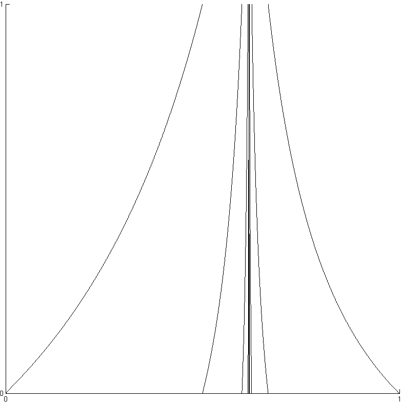
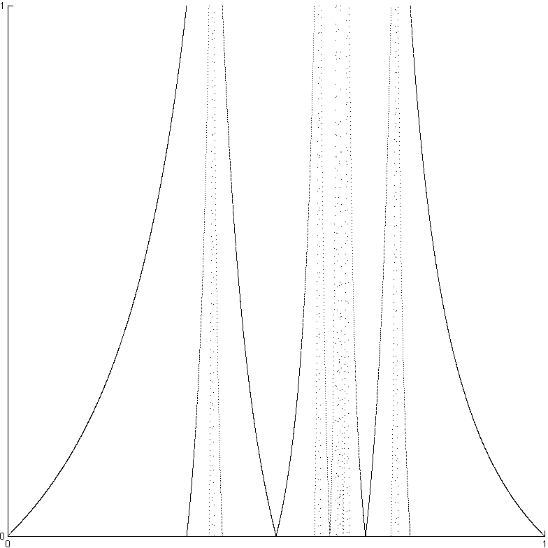
4.3 The graph of jimm

Since \RLj𝐑subscript\RLj𝐑{\leavevmode\hbox{\raise 4.30554pt\hbox{\set@color\resizebox{}{}{\scalebox{0.8}[0.8]{{\leavevmode\hbox{\hskip 0.0pt\lower-0.19293pt\hbox{\set@color{\RL{j}}}}}}}}}}_{\mathbf{R}} has a non-removable discontinuity at every rational point, it is not possible to draw its graph in the usual way. Below is a computer-produced box-graph of \RLj(x)\RLj𝑥{\leavevmode\hbox{\raise 4.30554pt\hbox{\set@color\resizebox{}{}{\scalebox{0.8}[0.8]{{\leavevmode\hbox{\hskip 0.0pt\lower-0.19293pt\hbox{\set@color{\RL{j}}}}}}}}}}(x) for $x\geq 0$, the graph lies inside the smaller (and darker) boxes.

This graph is found as follows. If $x\in(1,2)$, then $x=[1,n_{1},r]$ with $r\in(1,\infty)$, and there are two cases

$$x\in(1,\infty)=\bigcup_{n_{0}=1}^{\infty}(n_{0},\infty)\iff x=[n_{0},r]\mbox{ with }n_{0}\geq 1,\mbox{ and }r\in(1,\infty)$$
$\displaystyle(n_{0}\geq 1),\quad x\in(n_{0},n_{0}+1)=\bigcup_{n_{1}=1}^{\infty}\left[n_{0}+\frac{1}{n_{1}+1},n_{0}+\frac{1}{n_{1}}\right]$
$\displaystyle x=[n_{0},n_{1},r]\mbox{ with }n_{1}\geq 1,\quad 1<r<\infty$
\RLj(x)=[1,1,,1n01times,m1,1,1,,1n12times,,1,2,],absent\RLj𝑥subscript111subscript𝑛01𝑡𝑖𝑚𝑒𝑠subscript𝑚1subscript111subscript𝑛12𝑡𝑖𝑚𝑒𝑠12\displaystyle\implies{\leavevmode\hbox{\raise 4.30554pt\hbox{\set@color\resizebox{}{}{\scalebox{0.8}[0.8]{{\leavevmode\hbox{\hskip 0.0pt\lower-0.19293pt\hbox{\set@color{\RL{j}}}}}}}}}}(x)=[\underbrace{1,1,\dots,1}_{n_{0}-1\,times},m_{1},\underbrace{1,1,\dots,1}_{n_{1}-2\,times},\dots,1,2,\dots],

where $m_{1}$=2 if $n_{1}>1$ and $m_{1}\geq 3$ if $n_{1}=1$. So in any case, $m_{1}\geq 2$, so that

(n01),x(n0,n0+1)\RLj(x)[1,1,,1n01times,[2,]]subscript𝑛01𝑥subscript𝑛0subscript𝑛01\RLj𝑥subscript111subscript𝑛01𝑡𝑖𝑚𝑒𝑠2(n_{0}\geq 1),\quad x\in(n_{0},n_{0}+1)\implies{\leavevmode\hbox{\raise 4.30554pt\hbox{\set@color\resizebox{}{}{\scalebox{0.8}[0.8]{{\leavevmode\hbox{\hskip 0.0pt\lower-0.19293pt\hbox{\set@color{\RL{j}}}}}}}}}}(x)\in[\underbrace{1,1,\dots,1}_{n_{0}-1\,times},[2,\infty]]

In other words,

(n02),\RLj((n0,n0+1))=[Fn0+3Fn0+2,Fn0+1Fn0]subscript𝑛02\RLjsubscript𝑛0subscript𝑛01subscript𝐹subscript𝑛03subscript𝐹subscript𝑛02subscript𝐹subscript𝑛01subscript𝐹subscript𝑛0(n_{0}\geq 2),\implies\quad{\leavevmode\hbox{\raise 4.30554pt\hbox{\set@color\resizebox{}{}{\scalebox{0.8}[0.8]{{\leavevmode\hbox{\hskip 0.0pt\lower-0.19293pt\hbox{\set@color{\RL{j}}}}}}}}}}((n_{0},n_{0}+1))=\left[\frac{F_{n_{0}+3}}{F_{n_{0}+2}},\frac{F_{n_{0}+1}}{F_{n_{0}}}\right]

(intervals being inverted depending on the parity of $n_{0}$). Now suppose that $x\in[2,3)$. Continuing in this manner gives the following graph:

[Uncaptioned image]

The graph on the negative sector can be found by using the functional equation \RLj(x)=1/\RLj(x)\RLj𝑥1\RLj𝑥{\leavevmode\hbox{\raise 4.30554pt\hbox{\set@color\resizebox{}{}{\scalebox{0.8}[0.8]{{\leavevmode\hbox{\hskip 0.0pt\lower-0.19293pt\hbox{\set@color{\RL{j}}}}}}}}}}(-x)=-1/{\leavevmode\hbox{\raise 4.30554pt\hbox{\set@color\resizebox{}{}{\scalebox{0.8}[0.8]{{\leavevmode\hbox{\hskip 0.0pt\lower-0.19293pt\hbox{\set@color{\RL{j}}}}}}}}}}(x).

5 Action on the quadratic irrationalities

Since \RLjsubscript\RLj{\leavevmode\hbox{\raise 4.30554pt\hbox{\set@color\resizebox{}{}{\scalebox{0.8}[0.8]{{\leavevmode\hbox{\hskip 0.0pt\lower-0.19293pt\hbox{\set@color{\RL{j}}}}}}}}}}_{\mathcal{F}} sends eventually periodic paths to eventually periodic paths, \RLj𝐑subscript\RLj𝐑{\leavevmode\hbox{\raise 4.30554pt\hbox{\set@color\resizebox{}{}{\scalebox{0.8}[0.8]{{\leavevmode\hbox{\hskip 0.0pt\lower-0.19293pt\hbox{\set@color{\RL{j}}}}}}}}}}_{\mathbf{R}} preserves the real-multiplication set. This is the content of our next result:

Theorem 18

\RLj defines an involution of the set of real quadratic irrationals, (including rationals) and it respects the $\mathrm{PGL}_{2}(\mathbf{Z})$-orbits.

Beyond this theorem, we failed to detect any further arithmetic structure or formula relating the quadratic number to its \RLj -transform. All we can do is to give some sporadic examples, which amounts to exhibit some special real quadratic numbers with known continued fraction expansions. We shall do this below. Before that, however, note that the equation below is solvable for every $n\in\mathbf{Z}$:

\RLjx=n+xx=

\RLj

\RLj

x
=T~n\RLjxx=T~n(x+n)
\RLj𝑥𝑛𝑥𝑥

\RLj

\RLj

𝑥
superscript~𝑇𝑛\RLj𝑥𝑥superscript~𝑇𝑛𝑥𝑛
{\leavevmode\hbox{\raise 4.30554pt\hbox{\set@color\resizebox{}{}{\scalebox{0.8}[0.8]{{\leavevmode\hbox{\hskip 0.0pt\lower-0.19293pt\hbox{\set@color{\RL{j}}}}}}}}}}x=n+x\implies x={\leavevmode\hbox{\raise 4.30554pt\hbox{\set@color\resizebox{}{}{\scalebox{0.8}[0.8]{{\leavevmode\hbox{\hskip 0.0pt\lower-0.19293pt\hbox{\set@color{\RL{j}}}}}}}}}}{\leavevmode\hbox{\raise 4.30554pt\hbox{\set@color\resizebox{}{}{\scalebox{0.8}[0.8]{{\leavevmode\hbox{\hskip 0.0pt\lower-0.19293pt\hbox{\set@color{\RL{j}}}}}}}}}}x=\widetilde{T}^{n}{\leavevmode\hbox{\raise 4.30554pt\hbox{\set@color\resizebox{}{}{\scalebox{0.8}[0.8]{{\leavevmode\hbox{\hskip 0.0pt\lower-0.19293pt\hbox{\set@color{\RL{j}}}}}}}}}}x\implies x=\widetilde{T}^{n}(x+n)
$$\frac{F_{n+1}(x+n)+F_{n}}{F_{n}(x+n)+F_{n-1}}=x=\frac{F_{n+1}x+F_{n}+nF_{n+1}}{F_{n}x^{n}+F_{n-1}+nF_{n}}$$
$$\implies F_{n}x^{2}+(F_{n-1}+nF_{n}-F_{n+1})x-(F_{n}+nF_{n+1})$$

More generally, the equation \RLjx=Mx\RLj𝑥𝑀𝑥{\leavevmode\hbox{\raise 4.30554pt\hbox{\set@color\resizebox{}{}{\scalebox{0.8}[0.8]{{\leavevmode\hbox{\hskip 0.0pt\lower-0.19293pt\hbox{\set@color{\RL{j}}}}}}}}}}x=Mx is solvable for $M\in\mathrm{PGL}_{2}(\mathbf{Z})$. Indeed one has

\RLjx=Mxx=

\RLj

\RLj

x
=(\RLjM)(\RLjx)=(\RLjM)Mx
,
\RLj𝑥𝑀𝑥𝑥

\RLj

\RLj

𝑥
\RLj𝑀\RLj𝑥\RLj𝑀𝑀𝑥
{\leavevmode\hbox{\raise 4.30554pt\hbox{\set@color\resizebox{}{}{\scalebox{0.8}[0.8]{{\leavevmode\hbox{\hskip 0.0pt\lower-0.19293pt\hbox{\set@color{\RL{j}}}}}}}}}}x=Mx\implies x={\leavevmode\hbox{\raise 4.30554pt\hbox{\set@color\resizebox{}{}{\scalebox{0.8}[0.8]{{\leavevmode\hbox{\hskip 0.0pt\lower-0.19293pt\hbox{\set@color{\RL{j}}}}}}}}}}{\leavevmode\hbox{\raise 4.30554pt\hbox{\set@color\resizebox{}{}{\scalebox{0.8}[0.8]{{\leavevmode\hbox{\hskip 0.0pt\lower-0.19293pt\hbox{\set@color{\RL{j}}}}}}}}}}x=({\leavevmode\hbox{\raise 4.30554pt\hbox{\set@color\resizebox{}{}{\scalebox{0.8}[0.8]{{\leavevmode\hbox{\hskip 0.0pt\lower-0.19293pt\hbox{\set@color{\RL{j}}}}}}}}}}M)({\leavevmode\hbox{\raise 4.30554pt\hbox{\set@color\resizebox{}{}{\scalebox{0.8}[0.8]{{\leavevmode\hbox{\hskip 0.0pt\lower-0.19293pt\hbox{\set@color{\RL{j}}}}}}}}}}x)=({\leavevmode\hbox{\raise 4.30554pt\hbox{\set@color\resizebox{}{}{\scalebox{0.8}[0.8]{{\leavevmode\hbox{\hskip 0.0pt\lower-0.19293pt\hbox{\set@color{\RL{j}}}}}}}}}}M)Mx,

and the solutions are the fixed points of (\RLjM)M\RLj𝑀𝑀({\leavevmode\hbox{\raise 4.30554pt\hbox{\set@color\resizebox{}{}{\scalebox{0.8}[0.8]{{\leavevmode\hbox{\hskip 0.0pt\lower-0.19293pt\hbox{\set@color{\RL{j}}}}}}}}}}M)M. These points are precisely the words represented by the infinite path

x=(\RLjM)M(\RLjM)M(\RLjM)M(\RLjM)M𝑥\RLj𝑀𝑀\RLj𝑀𝑀\RLj𝑀𝑀\RLj𝑀𝑀\displaystyle x=({\leavevmode\hbox{\raise 4.30554pt\hbox{\set@color\resizebox{}{}{\scalebox{0.8}[0.8]{{\leavevmode\hbox{\hskip 0.0pt\lower-0.19293pt\hbox{\set@color{\RL{j}}}}}}}}}}M)M({\leavevmode\hbox{\raise 4.30554pt\hbox{\set@color\resizebox{}{}{\scalebox{0.8}[0.8]{{\leavevmode\hbox{\hskip 0.0pt\lower-0.19293pt\hbox{\set@color{\RL{j}}}}}}}}}}M)M({\leavevmode\hbox{\raise 4.30554pt\hbox{\set@color\resizebox{}{}{\scalebox{0.8}[0.8]{{\leavevmode\hbox{\hskip 0.0pt\lower-0.19293pt\hbox{\set@color{\RL{j}}}}}}}}}}M)M({\leavevmode\hbox{\raise 4.30554pt\hbox{\set@color\resizebox{}{}{\scalebox{0.8}[0.8]{{\leavevmode\hbox{\hskip 0.0pt\lower-0.19293pt\hbox{\set@color{\RL{j}}}}}}}}}}M)M\dots (25)

where we assume that both $M$ and \RLjM\RLj𝑀{\leavevmode\hbox{\raise 4.30554pt\hbox{\set@color\resizebox{}{}{\scalebox{0.8}[0.8]{{\leavevmode\hbox{\hskip 0.0pt\lower-0.19293pt\hbox{\set@color{\RL{j}}}}}}}}}}M are expressed as words in $U$ and $T$. Note that these words are precisely the points whose conjugacy classes remain stable under \RLj .

\RLjx=M(\RLjM)M(\RLjM)M(\RLjM)M(\RLjM)M\RLj𝑥𝑀\RLj𝑀𝑀\RLj𝑀𝑀\RLj𝑀𝑀\RLj𝑀𝑀{\leavevmode\hbox{\raise 4.30554pt\hbox{\set@color\resizebox{}{}{\scalebox{0.8}[0.8]{{\leavevmode\hbox{\hskip 0.0pt\lower-0.19293pt\hbox{\set@color{\RL{j}}}}}}}}}}x=M({\leavevmode\hbox{\raise 4.30554pt\hbox{\set@color\resizebox{}{}{\scalebox{0.8}[0.8]{{\leavevmode\hbox{\hskip 0.0pt\lower-0.19293pt\hbox{\set@color{\RL{j}}}}}}}}}}M)M({\leavevmode\hbox{\raise 4.30554pt\hbox{\set@color\resizebox{}{}{\scalebox{0.8}[0.8]{{\leavevmode\hbox{\hskip 0.0pt\lower-0.19293pt\hbox{\set@color{\RL{j}}}}}}}}}}M)M({\leavevmode\hbox{\raise 4.30554pt\hbox{\set@color\resizebox{}{}{\scalebox{0.8}[0.8]{{\leavevmode\hbox{\hskip 0.0pt\lower-0.19293pt\hbox{\set@color{\RL{j}}}}}}}}}}M)M({\leavevmode\hbox{\raise 4.30554pt\hbox{\set@color\resizebox{}{}{\scalebox{0.8}[0.8]{{\leavevmode\hbox{\hskip 0.0pt\lower-0.19293pt\hbox{\set@color{\RL{j}}}}}}}}}}M)M\dots

One may also view these numbers $x$ as sort of eigenvectors of the \RLj operator: \RLj(x)=M\RLj(x)\RLj𝑥𝑀\RLj𝑥{\leavevmode\hbox{\raise 4.30554pt\hbox{\set@color\resizebox{}{}{\scalebox{0.8}[0.8]{{\leavevmode\hbox{\hskip 0.0pt\lower-0.19293pt\hbox{\set@color{\RL{j}}}}}}}}}}(x)=M{\leavevmode\hbox{\raise 4.30554pt\hbox{\set@color\resizebox{}{}{\scalebox{0.8}[0.8]{{\leavevmode\hbox{\hskip 0.0pt\lower-0.19293pt\hbox{\set@color{\RL{j}}}}}}}}}}(x).

Hence the $\mathrm{PGL}_{2}(\mathbf{Z})$-orbits of the points in (25) remain stable under \RLj . Since the set of these orbits is the moduli space of real lattices, we deduce the result:

Proposition 19

The fixed points of the involution \RLj on the moduli space of real lattices are precisely the points (25) .

For example, if \RLjM=T~k+1\RLj𝑀superscript~𝑇𝑘1{\leavevmode\hbox{\raise 4.30554pt\hbox{\set@color\resizebox{}{}{\scalebox{0.8}[0.8]{{\leavevmode\hbox{\hskip 0.0pt\lower-0.19293pt\hbox{\set@color{\RL{j}}}}}}}}}}M=\widetilde{T}^{k+1} then $M=T^{k+1}$, and the point (25) is nothing but the point $[\overline{1_{k},k+2}]$ mentioned in the introduction.


Example.

In [44] it is shown that

$$x=[0;{\overline{1_{n-1},a}}]=\frac{a}{2}\left(\sqrt{1+4\frac{aF_{n-1}+F_{n-2}}{a^{2}F_{n}}}-1\right)$$

Hence \RLj(x)=[0;n,a2,n+1¯],and\RLj𝑥0𝑛¯𝑎2𝑛1𝑎𝑛𝑑{\leavevmode\hbox{\raise 4.30554pt\hbox{\set@color\resizebox{}{}{\scalebox{0.8}[0.8]{{\leavevmode\hbox{\hskip 0.0pt\lower-0.19293pt\hbox{\set@color{\RL{j}}}}}}}}}}(x)=[0;n,\overline{a-2,n+1}],and so \RLj(x)=(n+1y)1,\RLj𝑥superscript𝑛1𝑦1{\leavevmode\hbox{\raise 4.30554pt\hbox{\set@color\resizebox{}{}{\scalebox{0.8}[0.8]{{\leavevmode\hbox{\hskip 0.0pt\lower-0.19293pt\hbox{\set@color{\RL{j}}}}}}}}}}(x)=({n+\frac{1}{y}})^{-1}, where

$$y=\frac{(a-2)(n+1)+\sqrt{(a-2)^{2}(n+1)^{2}+4(a-2)(n+1)}}{2(n+1)}.$$
Example.

(From Einsiedler & Ward [15], Pg.90, ex. 3.1.1) This result of McMullen from [34] illustrates how \RLj behaves on one real quadratic number field. $\mathbf{Q}(\sqrt{5})$ contains infinitely many elements with a uniform bound on their partial quotients, since $[\overline{1_{k+1},4,5,1_{k},3}]\in\mathbf{Q}(\sqrt{5}),\quad\forall k=1,2,\dots.$ Routine calculations shows that the transforms \RLj([1k+1,4,5,1k,3¯])=[k+2,2,2,3,k+2,1,k+3¯]\RLjdelimited-[]¯subscript1𝑘145subscript1𝑘3𝑘2¯223𝑘21𝑘3{\leavevmode\hbox{\raise 4.30554pt\hbox{\set@color\resizebox{}{}{\scalebox{0.8}[0.8]{{\leavevmode\hbox{\hskip 0.0pt\lower-0.19293pt\hbox{\set@color{\RL{j}}}}}}}}}}([\overline{1_{k+1},4,5,1_{k},3}])=[k+2,\overline{2,2,3,k+2,1,k+3}] lies in different quadratic number fields for different $k$’s. Hence, not only \RLj does not preserve the property of “belonging to a certain quadratic number field”, it sends elements from one quadratic number field to different quadratic number fields. The following result provides even more examples of this nature:

Theorem 20

(McMullen [34]) For any $s>0$, the periodic continued fractions

$$x_{m}=[\overline{(1,s)^{m},1,s+1,s-1,(1,s)^{m},1,s+1,s+3)}]$$

lie in $\mathbf{Q}(\sqrt{s^{2}+4s})$ for any $m\geq 0$.

The fact recently shown by McMullen is that $\mathbf{Q}(\sqrt{d})$ contains infinitely elements with partial quotients bounded by some number $M_{d}$. He also raises the question: can one take $M_{d}=2$?

Example 4 (Powers of the golden ratio)
Theorem 21

(Fishman and Miller [17]) One has the following

$$\Phi^{k}=\begin{cases}[\overline{F_{k+1}+F_{k-1}}],&\mbox{\it if k is even},\\ [F_{k+1}+F_{k-1}-1,\overline{1,F_{k+1}+F_{k-1}-2}]&\mbox{\it if k is odd}.\end{cases}$$
Corollary 22

The continued fraction of the kth power of the golden section is

\RLj(Φk)={[1Fk+1+Fk11,2,1Fk+1+Fk12¯],if k is even,[1Fk+1+Fk12,3,1Fk+1+Fk14¯]if k is odd.\RLjsuperscriptΦ𝑘casessubscript1subscript𝐹𝑘1subscript𝐹𝑘11¯2subscript1subscript𝐹𝑘1subscript𝐹𝑘12if k is evensubscript1subscript𝐹𝑘1subscript𝐹𝑘12¯3subscript1subscript𝐹𝑘1subscript𝐹𝑘14if k is odd{\leavevmode\hbox{\raise 4.30554pt\hbox{\set@color\resizebox{}{}{\scalebox{0.8}[0.8]{{\leavevmode\hbox{\hskip 0.0pt\lower-0.19293pt\hbox{\set@color{\RL{j}}}}}}}}}}(\Phi^{k})=\begin{cases}[1_{F_{k+1}+F_{k-1}-1},\overline{2,1_{F_{k+1}+F_{k-1}-2}}],&\mbox{\it if k is even},\\ [1_{F_{k+1}+F_{k-1}-2},\overline{3,1_{F_{k+1}+F_{k-1}-4}}]&\mbox{\it if k is odd}.\end{cases}

The following generalization of this is also known:

Theorem 23

(Fishman and Miller [17]) Consider the recurrence relation

$$g_{n+1}=mg_{n}+lg_{n-1},\mbox{ with }g_{0}=0,g_{1}=1,\quad,m\in\mathbf{Z}_{>0},\quad l=\pm 1.$$

Let

$$\Phi_{m,l}:=\lim_{n\rightarrow\infty}\frac{g_{n}}{g_{n}-1}=\frac{m\pm\sqrt{m^{2}+4l}}{2}.$$

Then for any positive integer $k$, if $l=1$ one has

$$\Phi_{m,1}^{k}=\begin{cases}[\overline{g_{k+1}+g_{k-1}}],&\mbox{\it if k is odd},\\ [g_{k+1}+g_{k-1}-1,\overline{1,g_{k+1}+g_{k-1}-2}]&\mbox{\it if k is odd},\end{cases}$$

while if $l=1$ one has

$$\Phi_{m,-1}^{k}=[g_{k+1}-g_{k-1}-1,\overline{1,g_{k+1}-g_{k-1}-2}]\quad\mbox{\it if k is odd},$$

We leave it to the reader to determine the \RLj -transform of $\Phi_{m,l}^{k}$.

Example.

Suppose $\alpha=p+\sqrt{q}$ be a quadratic irrational with $p,q\in\mathbf{Q}$. Then $\alpha^{*}=1/\alpha$ provided

$$|\alpha|^{2}=p^{2}-q=1\implies q=p^{2}-1.$$

Suppose $\alpha$ is of this form, i.e. $\alpha=p+\sqrt{p^{2}-1}$ and suppose \RLj(α)=x+y\RLj𝛼𝑥𝑦{\leavevmode\hbox{\raise 4.30554pt\hbox{\set@color\resizebox{}{}{\scalebox{0.8}[0.8]{{\leavevmode\hbox{\hskip 0.0pt\lower-0.19293pt\hbox{\set@color{\RL{j}}}}}}}}}}(\alpha)=x+\sqrt{y}. Then since

xy=\RLj(α)=\RLj(α)=\RLj(1/α)=1/\RLj(α)=1/(x+y)x2y=1,𝑥𝑦\RLjsuperscript𝛼\RLjsuperscript𝛼\RLj1𝛼1\RLj𝛼1𝑥𝑦superscript𝑥2𝑦1x-\sqrt{y}={\leavevmode\hbox{\raise 4.30554pt\hbox{\set@color\resizebox{}{}{\scalebox{0.8}[0.8]{{\leavevmode\hbox{\hskip 0.0pt\lower-0.19293pt\hbox{\set@color{\RL{j}}}}}}}}}}(\alpha)^{*}={\leavevmode\hbox{\raise 4.30554pt\hbox{\set@color\resizebox{}{}{\scalebox{0.8}[0.8]{{\leavevmode\hbox{\hskip 0.0pt\lower-0.19293pt\hbox{\set@color{\RL{j}}}}}}}}}}(\alpha^{*})={\leavevmode\hbox{\raise 4.30554pt\hbox{\set@color\resizebox{}{}{\scalebox{0.8}[0.8]{{\leavevmode\hbox{\hskip 0.0pt\lower-0.19293pt\hbox{\set@color{\RL{j}}}}}}}}}}(1/\alpha)=1/{\leavevmode\hbox{\raise 4.30554pt\hbox{\set@color\resizebox{}{}{\scalebox{0.8}[0.8]{{\leavevmode\hbox{\hskip 0.0pt\lower-0.19293pt\hbox{\set@color{\RL{j}}}}}}}}}}(\alpha)=1/(x+\sqrt{y})\implies x^{2}-y=1,

and we conclude that \RLj(α)\RLj𝛼{\leavevmode\hbox{\raise 4.30554pt\hbox{\set@color\resizebox{}{}{\scalebox{0.8}[0.8]{{\leavevmode\hbox{\hskip 0.0pt\lower-0.19293pt\hbox{\set@color{\RL{j}}}}}}}}}}(\alpha) is again of the form $x+\sqrt{x^{2}-1}$.

On the other hand, suppose \RLj(q)=x+y\RLj𝑞𝑥𝑦{\leavevmode\hbox{\raise 4.30554pt\hbox{\set@color\resizebox{}{}{\scalebox{0.8}[0.8]{{\leavevmode\hbox{\hskip 0.0pt\lower-0.19293pt\hbox{\set@color{\RL{j}}}}}}}}}}(\sqrt{q})=x+\sqrt{y}. Then

\RLj(q)=\RLj(q)=\RLj(q)=1/\RLj(q)|\RLj(q)|=x2y=1\RLjsuperscript𝑞\RLjsuperscript𝑞\RLj𝑞1\RLj𝑞\RLjsuperscript𝑞superscript𝑥2𝑦1{\leavevmode\hbox{\raise 4.30554pt\hbox{\set@color\resizebox{}{}{\scalebox{0.8}[0.8]{{\leavevmode\hbox{\hskip 0.0pt\lower-0.19293pt\hbox{\set@color{\RL{j}}}}}}}}}}(\sqrt{q})^{*}={\leavevmode\hbox{\raise 4.30554pt\hbox{\set@color\resizebox{}{}{\scalebox{0.8}[0.8]{{\leavevmode\hbox{\hskip 0.0pt\lower-0.19293pt\hbox{\set@color{\RL{j}}}}}}}}}}(\sqrt{q}^{*})={\leavevmode\hbox{\raise 4.30554pt\hbox{\set@color\resizebox{}{}{\scalebox{0.8}[0.8]{{\leavevmode\hbox{\hskip 0.0pt\lower-0.19293pt\hbox{\set@color{\RL{j}}}}}}}}}}(-\sqrt{q})=-1/{\leavevmode\hbox{\raise 4.30554pt\hbox{\set@color\resizebox{}{}{\scalebox{0.8}[0.8]{{\leavevmode\hbox{\hskip 0.0pt\lower-0.19293pt\hbox{\set@color{\RL{j}}}}}}}}}}(\sqrt{q})\implies|{\leavevmode\hbox{\raise 4.30554pt\hbox{\set@color\resizebox{}{}{\scalebox{0.8}[0.8]{{\leavevmode\hbox{\hskip 0.0pt\lower-0.19293pt\hbox{\set@color{\RL{j}}}}}}}}}}(\sqrt{q}^{*})|=x^{2}-y=-1

Hence, \RLj(q)\RLj𝑞{\leavevmode\hbox{\raise 4.30554pt\hbox{\set@color\resizebox{}{}{\scalebox{0.8}[0.8]{{\leavevmode\hbox{\hskip 0.0pt\lower-0.19293pt\hbox{\set@color{\RL{j}}}}}}}}}}(\sqrt{q}) is of the form $x+\sqrt{1+x^{2}}$. Conversely, if $\alpha$ is of the form $p+\sqrt{p^{2}+1}$, then \RLj(α)\RLj𝛼{\leavevmode\hbox{\raise 4.30554pt\hbox{\set@color\resizebox{}{}{\scalebox{0.8}[0.8]{{\leavevmode\hbox{\hskip 0.0pt\lower-0.19293pt\hbox{\set@color{\RL{j}}}}}}}}}}(\alpha) is a quadratic surd.

6 Statistics

By the Gauss-Kuzmin theorem, for almost all real numbers $x$, the frequency of an integer $k>0$ in the continued fraction expansion of $x$ converges to

$$\frac{1}{\log 2}\log\left(1+{1\over k(k+2)}\right)$$

(see [21]). We say that $x$ obeys the Gauss-Kuzmin statistics if this is the case.

If $X\in[0,1]$ is a uniformly distributed random variable, then almost everywhere the arithmetic mean of its partial quotients tends to infinity, i.e. if $X=[0,n_{1},n_{2},\dots]$ then

$$\lim_{k\to\infty}{n_{1}+\cdots+n_{k}\over k}=\infty\qquad\hbox{(a.s.)}$$ (26)

(see [21]). In other words, the set of numbers in the unit interval such that the above limit is infinite, is of full Lebesgue measure. Denote this set by $A$.

Now since the first $k$ partial fractions of $X$ give rise to at most $n_{1}+\cdots+n_{k}-k$ partial fractions of \RLj(X)\RLj𝑋{\leavevmode\hbox{\raise 4.30554pt\hbox{\set@color\resizebox{}{}{\scalebox{0.8}[0.8]{{\leavevmode\hbox{\hskip 0.0pt\lower-0.19293pt\hbox{\set@color{\RL{j}}}}}}}}}}(X) and at least $n_{1}+\cdots+n_{k}-2k$ of these are 1’s, one has

$${n_{1}+\cdots+n_{k}-k\over n_{1}+\cdots+n_{k}-2k}\to{\frac{n_{1}+\cdots+n_{k}}{k}-1\over\frac{n_{1}+\cdots+n_{k}}{k}-2}\to 1$$
Lemma 24

The density of $1$’s in the continued fraction expansion of \RLj(X)\RLj𝑋{\leavevmode\hbox{\raise 4.30554pt\hbox{\set@color\resizebox{}{}{\scalebox{0.8}[0.8]{{\leavevmode\hbox{\hskip 0.0pt\lower-0.19293pt\hbox{\set@color{\RL{j}}}}}}}}}}(X) equals 1 a.e., and therefore the the continued fraction averages of \RLj(X)\RLj𝑋{\leavevmode\hbox{\raise 4.30554pt\hbox{\set@color\resizebox{}{}{\scalebox{0.8}[0.8]{{\leavevmode\hbox{\hskip 0.0pt\lower-0.19293pt\hbox{\set@color{\RL{j}}}}}}}}}}(X) tend to 1 a.e.

We conclude that \RLj(A)\RLj𝐴{\leavevmode\hbox{\raise 4.30554pt\hbox{\set@color\resizebox{}{}{\scalebox{0.8}[0.8]{{\leavevmode\hbox{\hskip 0.0pt\lower-0.19293pt\hbox{\set@color{\RL{j}}}}}}}}}}(A) is a set of zero measure. This says that, even though the involution \RLj is a fundamental symmetry of $\mathbf{R}$, many properties of reals are strongly biased under it, unlike the other fundamental involutions $U$, $V$ and $K$.

We leave open the questions such as: what is the distribution of the continued fraction entries of \RLj(X)\RLj𝑋{\leavevmode\hbox{\raise 4.30554pt\hbox{\set@color\resizebox{}{}{\scalebox{0.8}[0.8]{{\leavevmode\hbox{\hskip 0.0pt\lower-0.19293pt\hbox{\set@color{\RL{j}}}}}}}}}}(X), if we ignore the 1’s?

6.1 The derivative of jimm.

A function discontinuous on a dense subset of $[0,1]$ can not be differentiable everywhere on the residual set; it can be differentiable at most on a meager set (i.e. a countable union of nowhere dense sets), see Fort’s paper [18]. But meager does not mean negligible: There exists meager sets of full Lebesgue measure, and it was also exhibited in the location cited a function discontinuous at rationals and yet differentiable on a set of full measure. It turns out that \RLj is a function of this kind.

To see why, recall that average values of continued fraction elements tend to infinity almost everywhere. Let $a=[0,n_{1},n_{2},\dots]$ be a number with this property:

$$\lim_{k\to\infty}{n_{1}+\cdots+n_{k}\over k}=\infty.$$ (27)

Then for every constant $M$, there is some $k$ with $n_{1}+\dots+n_{k}>kM$. But then the \RLj - transform of the initial length-$k$ segment of $x$ is of length at least $kM-k$. Hence if $y$ is any number whose continued fraction expansion coincide with that of $x$ up to the place $k$, then the continued fraction \RLj(y)\RLj𝑦{\leavevmode\hbox{\raise 4.30554pt\hbox{\set@color\resizebox{}{}{\scalebox{0.8}[0.8]{{\leavevmode\hbox{\hskip 0.0pt\lower-0.19293pt\hbox{\set@color{\RL{j}}}}}}}}}}(y) coincide with that of \RLj(x)\RLj𝑥{\leavevmode\hbox{\raise 4.30554pt\hbox{\set@color\resizebox{}{}{\scalebox{0.8}[0.8]{{\leavevmode\hbox{\hskip 0.0pt\lower-0.19293pt\hbox{\set@color{\RL{j}}}}}}}}}}(x) at least up to the place $kM-k$. Since $kM-k$ is arbitrarily big compared to $k$, and since longer continued fractions give exponentially better approximations, we see that \RLj(y)\RLj𝑦{\leavevmode\hbox{\raise 4.30554pt\hbox{\set@color\resizebox{}{}{\scalebox{0.8}[0.8]{{\leavevmode\hbox{\hskip 0.0pt\lower-0.19293pt\hbox{\set@color{\RL{j}}}}}}}}}}(y) a.e. is much closer to \RLj(x)\RLj𝑥{\leavevmode\hbox{\raise 4.30554pt\hbox{\set@color\resizebox{}{}{\scalebox{0.8}[0.8]{{\leavevmode\hbox{\hskip 0.0pt\lower-0.19293pt\hbox{\set@color{\RL{j}}}}}}}}}}(x) then $y$ is to $x$. Hence the idea of the following theorem.

Theorem 25

The derivative of \RLj(a)\RLj𝑎{\leavevmode\hbox{\raise 4.30554pt\hbox{\set@color\resizebox{}{}{\scalebox{0.8}[0.8]{{\leavevmode\hbox{\hskip 0.0pt\lower-0.19293pt\hbox{\set@color{\RL{j}}}}}}}}}}(a) exists almost everywhere and vanishes almost everywhere.

To prove this, we need to show that for almost all $a$,

limxa\RLj(a)\RLj(x)ax=0.subscript𝑥𝑎\RLj𝑎\RLj𝑥𝑎𝑥0\lim_{x\to a}\frac{{\leavevmode\hbox{\raise 4.30554pt\hbox{\set@color\resizebox{}{}{\scalebox{0.8}[0.8]{{\leavevmode\hbox{\hskip 0.0pt\lower-0.19293pt\hbox{\set@color{\RL{j}}}}}}}}}}(a)-{\leavevmode\hbox{\raise 4.30554pt\hbox{\set@color\resizebox{}{}{\scalebox{0.8}[0.8]{{\leavevmode\hbox{\hskip 0.0pt\lower-0.19293pt\hbox{\set@color{\RL{j}}}}}}}}}}(x)}{a-x}=0.

Assume that $x$ is irrational or equivalently its continued fraction expansion is non-terminating.

Let $x\in[0,1]$ with $0<|x-a|<\delta$ for some $\delta$. Then there is a number $k=k_{\delta}$, such that the continued fractions of $a$ and $x$ coincide up to the $k$th element. Hence $x=[0,n_{1},n_{2},\dots n_{k},m_{k+1},\dots]\mbox{ with }m_{k+1}\neq n_{k+1}.$ Note that this latter condition also guarantees that $0<|x-a|$. Now let

$$M_{k}(z):=[n_{1},n_{2},\dots,n_{k-1},n_{k}+z]=\frac{\alpha_{k}z+\beta_{k}}{\gamma_{k}z+\theta_{k}}$$

and put $a_{k}:=[0,n_{k+1},n_{k+2},\dots],\quad x_{k}:=[0,m_{k+1},m_{k+2},\dots].$ Then one has $0<a_{k}<1$ (with strict inequality since $a$ is irrational) and $0\leq x_{k}<1$ for every $k=1,2,\dots$. One has

$$a=M_{k}(a_{k}),\quad x=M_{k}(x_{k})\mbox{ and }\det(M_{k})=(-1)^{k}.$$
Lemma 26

Let $a:=[0,n_{0},n_{1},\dots]$ and suppose that the continued fractions of $a$ and $x$ coincide up to the place $k$ (but not $k+1$), where $x\in[0,1]$. Put $N_{k}:=\sum_{i=1}^{k}n_{i}$, and $\mu_{k}:=N/k$. Then

$$|a-x|>\frac{1}{24}(2\mu_{k+3})^{-2(k+3)}$$

Proof. One has

$$|a-x|=\left|M_{k}(a_{k})-M_{k}(x_{k})\right|=\left|\frac{\alpha_{k}a_{k}+\beta_{k}}{\gamma_{k}a_{k}+\theta_{k}}-\frac{\alpha_{k}x_{k}+\beta_{k}}{\gamma_{k}x_{k}+\theta_{k}}\right|=\frac{1}{(\gamma_{k}a_{k}+\theta_{k})(\gamma_{k}x_{k}+\theta_{k}})$$

Since

$$M_{i+1}(z)=M_{i}\left(\frac{1}{n_{i+1}+z}\right)=\frac{\beta_{i}z+(\alpha_{i}+n_{i+1}\beta_{i})}{\theta_{i}z+(\gamma+n_{i+1}\theta_{i})},$$

one has $\gamma_{i+1}=\theta_{i}$ and $\theta_{i+1}=\gamma_{i}+n_{i+1}\theta_{i}$. Hence $\theta_{i+1}>\gamma_{i+1}\implies\theta_{i+1}>\theta_{i}(1+n_{i+1})$. This implies

$\displaystyle\theta_{i}<(1+n_{1})(1+n_{2})\dots(1+n_{i}),$
$\displaystyle\gamma_{i}<(1+n_{1})(1+n_{2})\dots(1+n_{i-1}).$

Since $0\leq a_{k},x_{k}<1$, this implies

$\displaystyle\gamma_{k}a_{k}+\theta_{k}<\gamma_{k}+\theta_{k}<2(1+n_{1})(1+n_{2})\dots(1+n_{k}),$
$\displaystyle\gamma_{k}x_{k}+\theta_{k}<\gamma_{k}+\theta_{k}<2(1+n_{1})(1+n_{2})\dots(1+n_{k}).$

Hence, we get

$$|a-x|>\frac{|a_{k}-x_{k}|}{4(1+n_{1})^{2}(1+n_{2})^{2}\dots(1+n_{k})^{2}}$$

To estimate $|a_{k}-x_{k}|$, consider

$$a_{k}-x_{k}=\frac{1}{n_{k+1}+a_{k+1}}-\frac{1}{m_{k+1}+x_{k+1}}=\frac{m_{k+1}-n_{k+1}+x_{k+1}-a_{k+1}}{(n_{k+1}+a_{k+1})(m_{k+1}+x_{k+1})}$$
$$>\frac{m_{k+1}-n_{k+1}+x_{k+1}-a_{k+1}}{(1+n_{k+1})(1+m_{k+1})}.$$

Now, if $m_{k+1}<n_{k+1}$ then set $m_{k+1}=n_{k+1}-t$ with $t\geq 1$. Then one has

$$|a_{k}-x_{k}|>\frac{|-t+x_{k+1}-a_{k+1}|}{(1+n_{k+1})(1+n_{k+1}-t)}>\frac{a_{k+1}}{(1+n_{k+1})^{2}}$$

On the other hand, if $3n_{k+1}\geq m_{k+1}>n_{k+1}$ then

$$|a_{k}-x_{k}|>\frac{|1+x_{k+1}-a_{k+1}|}{(1+n_{k+1})(1+3n_{k+1})}>\frac{1-a_{k+1}}{3(1+n_{k+1})^{2}},$$

and if $m_{k+1}>3n_{k+1}$ then

$$|a_{k}-x_{k}|=\frac{1-\frac{n_{k+1}}{m_{k+1}}+\frac{x_{k+1}}{m_{k+1}}-\frac{a_{k+1}}{m_{k+1}}}{(1+n_{k+1})(1+\frac{1}{m_{k+1}})}>\frac{1}{6(1+n_{k+1})}$$

So one has

$$|a_{k}-x_{k}|>\frac{a_{k+1}(1-a_{k+1})}{6(1+n_{k+1})^{2}},$$

which gives the estimation from below

$$|a-x|>\frac{a_{k+1}(1-a_{k+1})}{24(1+n_{1})^{2}(1+n_{2})^{2}\dots(1+n_{k})^{2}(1+n_{k+1})^{2}},$$

estimation obtained under the assumption that the continued fraction expansions of $x$ and $a$ coincide up until the $k$th term and differ for the $k+1$th term.

Now we have the crude estimate

$${\cfrac{1}{n_{k+2}+\cfrac{1}{n_{k+3}+1}}}>a_{k+1}>{1\over 1+n_{k+2}}\implies{a_{k+1}(1-a_{k+1})}>{1\over(1+n_{k+2})^{2}}{1\over(1+n_{k+3})^{2}}.$$

which gives

$$|a-x|>\frac{1}{24(1+n_{1})^{2}(1+n_{2})^{2}\dots(1+n_{k+2})^{2}(1+n_{k+3})^{2}},$$

Now put $N_{k}:=\sum_{i=1}^{k}n_{i}$, and $\mu_{k}:=N/k$. Then

$$(1+n_{1})^{2}(1+n_{2})^{2}\dots(1+n_{k})^{2}\leq(1+\mu_{k})^{2k}\leq(2\mu_{k})^{2k}$$

The last inequality follows from the fact that $\mu_{k}\geq 1$ for all $k$, since $n_{i}\geq 1$ for all $i$. We finally obtain the estimate

$$|a-x|>\frac{1}{24}(2\mu_{k+3})^{-2(k+3)}=\frac{1}{24}\exp\{-2(k+3)\log 2\mu_{k+3}\}$$

$\Box$

On the other hand, if the c.f. expansions of $a$ and $x$ coincide up to the $k=k(x)$th place, then the c.f. expansions of \RLj(a)\RLj𝑎{\leavevmode\hbox{\raise 4.30554pt\hbox{\set@color\resizebox{}{}{\scalebox{0.8}[0.8]{{\leavevmode\hbox{\hskip 0.0pt\lower-0.19293pt\hbox{\set@color{\RL{j}}}}}}}}}}(a) and \RLj(xi)\RLjsubscript𝑥𝑖{\leavevmode\hbox{\raise 4.30554pt\hbox{\set@color\resizebox{}{}{\scalebox{0.8}[0.8]{{\leavevmode\hbox{\hskip 0.0pt\lower-0.19293pt\hbox{\set@color{\RL{j}}}}}}}}}}(x_{i}) coincide up to the place $N_{k}$, and by (24) we have

|\RLj(a)\RLj(x)|<FNk2<5ϕ2Nk=5exp{2kμklogϕ}\RLj𝑎\RLj𝑥superscriptsubscript𝐹subscript𝑁𝑘25superscriptitalic-ϕ2subscript𝑁𝑘52𝑘subscript𝜇𝑘italic-ϕ|{\leavevmode\hbox{\raise 4.30554pt\hbox{\set@color\resizebox{}{}{\scalebox{0.8}[0.8]{{\leavevmode\hbox{\hskip 0.0pt\lower-0.19293pt\hbox{\set@color{\RL{j}}}}}}}}}}(a)-{\leavevmode\hbox{\raise 4.30554pt\hbox{\set@color\resizebox{}{}{\scalebox{0.8}[0.8]{{\leavevmode\hbox{\hskip 0.0pt\lower-0.19293pt\hbox{\set@color{\RL{j}}}}}}}}}}(x)|<F_{N_{k}}^{-2}<{\sqrt{5}}\phi^{-2N_{k}}={\sqrt{5}}\exp\{-2k\mu_{k}\log\phi\}

(This estimate should be close to optimal (a.e.), since the density of 1’s in the c.f. expansion of \RLj(a)\RLj𝑎{\leavevmode\hbox{\raise 4.30554pt\hbox{\set@color\resizebox{}{}{\scalebox{0.8}[0.8]{{\leavevmode\hbox{\hskip 0.0pt\lower-0.19293pt\hbox{\set@color{\RL{j}}}}}}}}}}(a) is 1 (a.e.) by Lemma 24.) This gives

|\RLj(a)\RLj(x)ax|<245expk{2(1+3/k)log2μk+32μklogϕ}\RLj𝑎\RLj𝑥𝑎𝑥245𝑘213𝑘2subscript𝜇𝑘32subscript𝜇𝑘italic-ϕabsent\left|\frac{{\leavevmode\hbox{\raise 4.30554pt\hbox{\set@color\resizebox{}{}{\scalebox{0.8}[0.8]{{\leavevmode\hbox{\hskip 0.0pt\lower-0.19293pt\hbox{\set@color{\RL{j}}}}}}}}}}(a)-{\leavevmode\hbox{\raise 4.30554pt\hbox{\set@color\resizebox{}{}{\scalebox{0.8}[0.8]{{\leavevmode\hbox{\hskip 0.0pt\lower-0.19293pt\hbox{\set@color{\RL{j}}}}}}}}}}(x)}{a-x}\right|<{24\sqrt{5}}\exp k\{2(1+3/k)\log 2\mu_{k+3}-2\mu_{k}\log\phi\}\implies
|\RLj(a)\RLj(x)ax|<Aexp{2klogϕ(Blog2μk+3μk)}\RLj𝑎\RLj𝑥𝑎𝑥𝐴2𝑘italic-ϕ𝐵2subscript𝜇𝑘3subscript𝜇𝑘\qquad\qquad\qquad\left|\frac{{\leavevmode\hbox{\raise 4.30554pt\hbox{\set@color\resizebox{}{}{\scalebox{0.8}[0.8]{{\leavevmode\hbox{\hskip 0.0pt\lower-0.19293pt\hbox{\set@color{\RL{j}}}}}}}}}}(a)-{\leavevmode\hbox{\raise 4.30554pt\hbox{\set@color\resizebox{}{}{\scalebox{0.8}[0.8]{{\leavevmode\hbox{\hskip 0.0pt\lower-0.19293pt\hbox{\set@color{\RL{j}}}}}}}}}}(x)}{a-x}\right|<A\exp\Bigl{\{}2k\log\phi\bigl{(}B\log 2\mu_{k+3}-\mu_{k}\bigr{)}\bigr{\}}

where $A$ is some absolute constant and $B=(1+3/k)/\log\phi$ can be taken arbitrarily close to $1/\log\phi<2.08$ by assuming $k$ is big enough.

We see immediately that, if $a=[0,n,n,n,n,\dots]$ then $\mu_{k}$ is constant $=n$, and if $n$ is taken big enough so that $2.08\log 2n-n<0$, then the derivative exists and is zero. This is true for $n>4$. We don’t claim that our estimations are optimal in this respect, however.

On the other hand, since $\mu_{k}\to\infty$ almost surely, we see that $B\log 2\mu_{k+3}-\mu_{k}<0$ for $k$ sufficiently big and the derivative exists and vanishes. This is because by choosing a sufficiently small neighborhood $\{|x-a|<\delta\}$, we can guarantee that $k=k(x)$ is always greater than a given number for any $x$ in this neighborhood. This concludes the proof of the theorem.

Note that, if $\mu_{k}\to\infty$ then the average of continued fraction elements of \RLj(a)\RLj𝑎{\leavevmode\hbox{\raise 4.30554pt\hbox{\set@color\resizebox{}{}{\scalebox{0.8}[0.8]{{\leavevmode\hbox{\hskip 0.0pt\lower-0.19293pt\hbox{\set@color{\RL{j}}}}}}}}}}(a) tends to 1, and \RLj is not differentiable at \RLj(a)\RLj𝑎{\leavevmode\hbox{\raise 4.30554pt\hbox{\set@color\resizebox{}{}{\scalebox{0.8}[0.8]{{\leavevmode\hbox{\hskip 0.0pt\lower-0.19293pt\hbox{\set@color{\RL{j}}}}}}}}}}(a). In other words, \RLj is almost surely not differentiable at \RLj(a)\RLj𝑎{\leavevmode\hbox{\raise 4.30554pt\hbox{\set@color\resizebox{}{}{\scalebox{0.8}[0.8]{{\leavevmode\hbox{\hskip 0.0pt\lower-0.19293pt\hbox{\set@color{\RL{j}}}}}}}}}}(a). In the same vein, the derivative of \RLj at $a=[0,n,n,n,n,\dots]$ vanish for $n>4$, and we see that \RLj is not differentiable at \RLj(a)=[0,1n1,2,n2¯]\RLj𝑎0subscript1𝑛1¯2𝑛2{\leavevmode\hbox{\raise 4.30554pt\hbox{\set@color\resizebox{}{}{\scalebox{0.8}[0.8]{{\leavevmode\hbox{\hskip 0.0pt\lower-0.19293pt\hbox{\set@color{\RL{j}}}}}}}}}}(a)=[0,1_{n-1},\overline{2,n-2}] or at best it will be of infinite slope at this point.

It might be of interest to study the derivatives at quadratic irrationalities in general. An exciting possibility would be to establish a connection with the derivative of \RLj and the Markov irrationalities, [2]. We don’t know if the derivative may attain or not a finite non-zero value at some point.

7 Concluding remarks.

7.1 The Minkowski measure and the Denjoy measures.

The reader with a taste for singular functions such as \RLj will inevitably ask how it relates to Minkowski’s question mark function. In our setting, this latter function is best understood as the cumulative distribution function of the unique $Aut_{I}(|\mathcal{F}|)$-invariant measure on the boundary $\partial\mathcal{F}$.

More generally888In a yet more general setting, , take any function $P:V_{\bullet}(\mathcal{F})\to[0,1]$ and let the random walker, upon arriving to a vertex, choose to turn right with probability $P(v)$ and to turn left with probability $1-P(v)$. Then this introduces a probability measure $\mu_{P}$ on $\partial\mathcal{F}$. A special class of measures is obtained, by requiring $P$ to be only a function of the distance to the starting edge. , let $p\in(0,1)$ be a real number. Suppose that a random walker on $\mathcal{F}$ starting at the edge $I$ decides with probability $1/2$ to move through the positive sector of $\mathcal{F}$ and then each time he arrives to a bifurcation, he chooses to turn right with probability $p$ and he chooses to turn left with probability $q:=1-p$. Similarly, he decides, with probability $1/2$ to move through the negative sector and then proceeds in the same manner at bifurcations. The probability that the walker ends up in the Farey interval ${\mathcal{O}}_{e^{\prime}}$ is the product of probabilities of choices he makes to go from the base edge $I$ to the edge $e^{\prime}$.

Note that, unlike the classical random walkers, ours is a non-backtracking walker. He is not allowed to retrace his steps (so this is not a Markov process) [41]. Since by definition the topology of the boundary is generated by the Farey intervals, this puts a measure on the Borel algebra of $\partial\mathcal{F}_{I}$ and since the quotient map $\partial\mathcal{F}_{I}\to S_{I}^{1}$ is measurable with respect to Borel algebras, we obtain a probability measure $\mu_{p}$ on $S_{I}^{1}$, the Denjoy measure first introduced and studied by Denjoy [10]. Since $0<p<1$, the set of rationals is of measure 0, so that this passage to the quotient has no detectable effect on the measure space properties. Let ${\mathbf{F}}_{p}(x)$ be the cumulative distribution function of $\mu_{p}$. Then ${\mathbf{F}}_{1/2}(x)$ is precisely the right extension of the Minkowski question mark function to $\widehat{\mathbf{R}}$ and provides a canonical homeomorphism $S_{I}^{1}\to[0,1]/0\!\sim\!1$ (recall that $\widehat{\mathbf{R}}$ is identified with $S_{I}^{1}$ by the continued fraction map $cfm$ and we may consider $\mu_{p}$ as a measure on $\widehat{\mathbf{R}}$ via this identification). As such, it conjugates the modular group to a group of homeomorphisms of $[0,1]/0\!\sim\!1$. The functional equations for the question mark function (see Alkauskas’ papers [4], [3]) then becomes a mere expression of this action. In fact, the conjugate representation of the modular group is a subgroup of Thompson’s group $T$ presented as the orientation preserving piecewise linear homeomorphisms of $[0,1]/0\!\sim\!1$ with break points at dyadic rationals and such that the slopes of linear pieces are all powers of 2, see [20]. Now ${\mathbf{F}}_{1/2}(x)$ also conjugates \RLj to an involution of $[0,1]/0\!\sim\!1$ (with jumps at dyadic rationals), and there are functional equations relating the action of this conjugate involution and the conjugate modular group action, similar to the ones we gave in the beginning of the paper. There is a possibility that this conjugate \RLj by the Minkowski function (or more generally by the functions ${\mathbf{F}}_{p}$) may interact in interesting ways with other singular functions such as the Takagi function[30]. See also the papers by Bonano and Isola [6], [5] for some more variations on this theme.

The measures $\mu_{p}$ are purely singular [52] with respect to the Lebesgue measure, i.e. their c.d.f’s ${\mathbf{F}}_{p}$ have a vanishing derivative almost everywhere, a property shared by the involution \RLj . In a different vein, it can be readily verified that the Minkowski measure999The measure $\mu_{1/2}$ have also been called the Lebesgue measure of $\partial\mathcal{F}$ ([9]) and also the Farey measure [27]. $\mu_{1/2}$ is an invariant measure for both the Gauss-Kuzming-Wirsing operator ${\mathscr{L}}^{G}_{2}$ (see the insightful paper of Vepstas [51]) and for the dual Gauss-Kuzming-Wirsing operator 2\RLjsubscriptsuperscript\RLj2{\mathscr{L}}^{{\leavevmode\hbox{\raise 3.01389pt\hbox{\set@color\resizebox{}{}{\scalebox{0.5}[0.5]{{\leavevmode\hbox{\hskip 0.0pt\lower-2.24292pt\hbox{\set@color{\RL{j}}}}}}}}}}}_{2}.

It seems that \RLj and ${\mathbf{F}}_{1/2}(x)$ recognize each other in another context: the integrals \RLj𝑑𝐅p(x)\RLjdifferential-dsubscript𝐅𝑝𝑥\int{\leavevmode\hbox{\raise 4.30554pt\hbox{\set@color\resizebox{}{}{\scalebox{0.8}[0.8]{{\leavevmode\hbox{\hskip 0.0pt\lower-0.19293pt\hbox{\set@color{\RL{j}}}}}}}}}}\,d{\mathbf{F}}_{p}(x) may well be finite.

7.2 Other trees and other continued fraction maps.

In fact, our story is about the group $\mathbf{Z}/2\mathbf{Z}*\mathbf{Z}/3\mathbf{Z}=\langle a,b\,|\,a^{2}=b^{3}=1\rangle$ and a certain representation of this group as a subgroup of ${\mathrm{PSL}}_{2}(\mathbf{R})$, namely the representation whose image is the modular group. Every representation gives rise to a sort of continued fraction map, with particularly nice properties if the element $ab$ is sent to a parabolic element. There are variations on this theme concerning the trees related to the free products $\mathbf{Z}/p\mathbf{Z}*\mathbf{Z}/q\mathbf{Z}\dots$ and their representations in ${\mathrm{PSL}}_{2}(\mathbf{R})$. The stories are particularly nice if the targets of the representations lies inside ${\mathrm{PGL}}_{2}(\mathbf{Q})$. Hecke groups (see [28],[29]) are also promising in this respect. These stories involve various \RLj -like automorphisms and boundary measures.

7.3 Covariant functions

As we already mentioned in the introduction, the functional equations satisfied by \RLj𝐑subscript\RLj𝐑{\leavevmode\hbox{\raise 4.30554pt\hbox{\set@color\resizebox{}{}{\scalebox{0.8}[0.8]{{\leavevmode\hbox{\hskip 0.0pt\lower-0.19293pt\hbox{\set@color{\RL{j}}}}}}}}}}_{\mathbf{R}} says that it lax-covariant with the action of $\mathrm{PGL}_{2}(\mathbf{Z})$ on $\widehat{\mathbf{R}}$. Is it possible to find some analytic function on the upper half plane satisfying those functional equations (if necessary after modifying them by the complex conjugation)?

On the other hand, there are some analytic $\mathrm{PSL}_{2}(\mathbf{Z})$-covariant functions on the upper half plane, discovered by Brady [8] and Smart [46], see the papers by Basraoui and Sebbar for a recent account (they use the term “equivariant” instead of “covariant”) [16] [43] [45]. The fact is that, if $h$ is an equivariant function (i.e. if $h$ satisfies the functional equations of \RLj ), then its Schwartzian is a weight-4 modular form. In the opposite direction, if $f$ is a weight-$k$ modular form, then the function

$$h(z)=z+k\frac{f(z)}{f^{\prime}(z)}$$

is $\mathrm{PSL}_{2}(\mathbf{Z})$-covariant. The $\kappa$ function of Kaneko and Yoshida [26] is covariant for an infinite subgroup of infinite index $\mathrm{PSL}_{2}(\mathbf{Z})$ (they use the word “covariant”). The Rogers-Ramanujan continued fraction $r(\tau)$ have some weak covariance properties, see [13]. Note that the identity function and the complex conjugation are $\mathrm{PSL}_{2}(\mathbf{Z})$- covariant, too.

We tried to concoct from \RLj𝐑subscript\RLj𝐑{\leavevmode\hbox{\raise 4.30554pt\hbox{\set@color\resizebox{}{}{\scalebox{0.8}[0.8]{{\leavevmode\hbox{\hskip 0.0pt\lower-0.19293pt\hbox{\set@color{\RL{j}}}}}}}}}}_{\mathbf{R}} a $\mathrm{PGL}_{2}(\mathbf{Z})$-invariant (singular) function on $\widehat{\mathbf{R}}$, but we failed.

7.4 Concepts similar to Jimm in Engineering

Digital communications implement some coding techniques to represent a data, and some signal conditioning transforms to obtain some desired properties on these representations. In analog communication when a carrier wave is used to transmit the data, as in the case of RF communications, a modulation of the carrier wave can be used to encode data; a sinusoidal carrier wave can be modulated in terms of its frequency, amplitude or phase. Be it RF, light, sound or electrical signals, the natural media used to transmit the digital information being analog, some discretizing mapping from digitally represented information to analog states is necessary.

Phase shift keying (PSK) is a modulation method to represent data in terms of changes of a sinusoidal carrier wave. When a modulation method assumes discrete values on modulated attribute of carrier wave, as in the case of digital communication, it is called “keying”, hence the name phase shift keying. Binary PSK assumes two distinct states of 180 degrees separated phases with equal amplitude and frequency; simplest binary to BPSK mapping is to represent a 0 bit in digital as a specific phase and, a 1 bit as the inverted phase. All signal are subject to mostly arbitrary phase shift during transmission (except in very controlled media like length balanced wires or PCB traces), unless the source and the receiver has another information source to decide which of two phases is the neutral one (i.e. 0 bit), PSK modulation suffers from what’s called phase ambiguity. Phase ambiguity can be addressed by supplying a non-modulated reference signal to compare the phase against (like a clock signal in digital electronics) which is not always practical; or by use of another transform on binary data called differential encoding. If a digital data is differentially encoded before PSK modulation, the each bit is not mapped to a specific phase of PSK states, but it is mapped to a specific change in phase. A differentially encoded data has the property called polarity insensitivity, which resolves the phase ambiguity issue (i.e. phone lines work no matter in which order the two copper wires are connected). Differential Manchester Encoding is a well known example of differential encoding which is used as the default encoding scheme of some versions of Ethernet (IEEE 802.3) computer network communications. Manchester encoding can also be thought of a digital counterpart of BPSK, it uses the digital clock signal to modulate the data signal via XOR operation; the resulting signal is same as the clock signal while the data bit (which is optionally differentially encoded before) is 0, and the inverse of clock signal if data bit is 1.

Jimm transformation of a number can be thought of being similar to BPSK; a number represented as zero and ones encoding the path on the farey tree, can be transformed using XOR operation to a modulation with a series of $(01)^{\omega}=010101..$. which serves like a carrier signal or digital clock. We face the same phase ambiguity issue as in the case of BPSK, but in this case the problem can be solved by means of convention, such as by mapping the left turns to 0 and right turns to 1, and not the other way, for farey tree encoding, and the carrier signal to be $(01)^{\omega}$ and not to $(10)^{\omega}$ thus fixing the neural phase to be carrier series starting with 0. There is no invariant signal (number) under this transformation, as carrier signal contains 1s and XORing with 1 is equivalent to negation which is an unary operator with no fixed point; but the signal (number) closest to be minimally changing under this transformation is $(0011)^{\omega}$ giving

$$(0011)^{\omega}\underline{\lor}(01)^{\omega}=011(0011)^{\omega}$$

which is the same signal 180 degrees out of phase, and the numbers related to $(0011)^{\omega}$ and $011(0011)^{\omega}$ are respectively $1+\sqrt{2}$ and $\sqrt{2}$.


Acknowledgements. We are grateful to Roelof Bruggeman, Alex Degtyarev, Gareth Jones, Masanobu Kaneko, Jeffrey Lagarias, Robert Langlands, Özer Öztürk, Recep Şahin, Susumu Tanabé, Michel Waldschmidt, Masaaki Yoshida, Mikhael Zaidenberg and Ayberk Zeytin for various suggestions, critiques and encouragement. We are thankful to the participants of the Ankara-İstanbul Algebraic Geometry and Number Theory Meetings who suffered the first exposition of the content of this paper.

This research have been supported by the Galatasaray University Research Grant 14.504.001 and the TÜBİTAK 1001 Grant No 110T690.

References

  • [1] Boris Adamczewski and Yann Bugeaud, Nombres réels de complexité sous-linéaire: mesures d’irrationalité et de transcendance, Journal für die reine und angewandte Mathematik (Crelles Journal) 2011 (2011), no. 658, 65–98.
  • [2] Martin Aigner, Markov’s theorem and 100 years of the uniqueness conjecture: a mathematical journey from irrational numbers to perfect matchings, Springer Science & Business Media, 2013.
  • [3] Giedrius Alkauskas, The minkowski question mark function: explicit series for the dyadic period function and moments, Mathematics of Computation 79 (2010), no. 269, 383–418.
  • [4]  , Semi-regular continued fractions and an exact formula for the moments of the minkowski question mark function, The Ramanujan Journal 25 (2011), no. 3, 359–367.
  • [5] Claudio Bonanno, Sandro Graffi, and Stefano Isola, Spectral analysis of transfer operators associated to farey fractions, arXiv preprint arXiv:0708.0686 (2007).
  • [6] Claudio Bonanno and Stefano Isola, Orderings of the rationals and dynamical systems, arXiv preprint arXiv:0805.2178 (2008).
  • [7]  , A thermodynamic approach to two-variable ruelle and selberg zeta functions via the farey map, Nonlinearity 27 (2014), no. 5, 897.
  • [8] Michael M Brady, Meromorphic solutions of a system of functional equations involving the modular group, Proceedings of the American Mathematical Society 30 (1971), no. 2, 271–277.
  • [9] Joel M Cohen, Flavia Colonna, and David Singman, Distributions and measures on the boundary of a tree, Journal of mathematical analysis and applications 293 (2004), no. 1, 89–107.
  • [10] Arnaud Denjoy, Sur une fonction réelle de minkowski, J. Math. Pures Appl 17 (1938), no. 9, 105.
  • [11] Warren Dicks and Martin John Dunwoody, Groups acting on graphs, vol. 17, Cambridge University Press, 1989.
  • [12] Dragomir Ž Djoković and Gary L Miller, Regular groups of automorphisms of cubic graphs, Journal of Combinatorial Theory, Series B 29 (1980), no. 2, 195–230.
  • [13] William Duke, Continued fractions and modular functions, Bulletin of the American Mathematical Society 42 (2005), no. 2, 137–162.
  • [14] Joan L Dyer, Automorphism sequences of integer unimodular groups, Illinois Journal of Mathematics 22 (1978), no. 1, 1–30.
  • [15] Manfred Einsiedler and Thomas Ward, Ergodic Theory: with a view towards Number Theory, vol. 259, Springer Verlag, 2010.
  • [16] Abdelkrim El Basraoui and Abdellah Sebbar, Rational equivariant forms, International Journal of Number Theory 8 (2012), no. 04, 963–981.
  • [17] Daniel Fishman and Steven J Miller, Closed form continued fraction expansions of special quadratic irrationals, ISRN Combinatorics 2013 (2013).
  • [18] MK Fort, A theorem concerning functions discontinuous on a dense set, American Mathematical Monthly (1951), 408–410.
  • [19] LK Hua and I Reiner, Automorphisms of the unimodular group, Transactions of the American Mathematical Society 71 (1951), no. 3, 331–348.
  • [20] Michel Imbert, Sur l’isomorphisme du groupe de richard thompson avec le groupe de ptolémée, LONDON MATHEMATICAL SOCIETY LECTURE NOTE SERIES (1997), 313–324.
  • [21] Marius Iosifescu and Cor Kraaikamp, Metrical theory of continued fractions, vol. 547, Springer Science & Business Media, 2002.
  • [22] Stefano Isola, Continued fractions and dynamics, Applied Mathematics 5 (2014), no. 07, 1067.
  • [23] Gareth A Jones and John S Thornton, Operations on maps, and outer automorphisms, Journal of Combinatorial Theory, Series B 35 (1983), no. 2, 93–103.
  • [24]  , Automorphisms and congruence subgroups of the extended modular group, Journal of the London Mathematical Society 2 (1986), no. 1, 26–40.
  • [25] Ken Kamano, Analytic continuation of the lucas zeta and l-functions, Indagationes Mathematicae 24 (2013), no. 3, 637–646.
  • [26] Masanobu Kaneko and Masaaki Yoshida, The kappa function, International Journal of Mathematics 14 (2003), no. 09, 1003–1013.
  • [27] Marc Kesseböhmer and Bernd O Stratmann, Fractal analysis for sets of non-differentiability of minkowski’s question mark function, Journal of Number Theory 128 (2008), no. 9, 2663–2686.
  • [28] Ozden Koruoglu and Recep Sahin, Generalized fibonacci sequences related to the extended hecke groups and an application to the extended modular group, Turk J Math 34 (2010), 325–332.
  • [29] Özden Koruoğlu, Recep Şahin, and Sebahattin İkikardeş, Trace Classes and Fixed Points for the Extended Modular Group, Turkish Journal of Mathematics 32 (2008), no. 1, 11–19.
  • [30] Jeffrey C Lagarias, The takagi function and its properties, arXiv preprint arXiv:1112.4205 (2011).
  • [31] J Lewis and Don Zagier, Period functions for maass wave forms. i, Annals of Mathematics 153 (2001), no. 1, 191–258.
  • [32] Yuri Manin and Matilde Marcolli, Modular shadows and the Levy-Mellin infinity-adic transform, arXiv preprint math/0703718 (2007).
  • [33] Dieter H Mayer, On the thermodynamic formalism for the gauss map, Communications in mathematical physics 130 (1990), no. 2, 311–333.
  • [34] Curtis T McMullen, Uniformly Diophantine numbers in a fixed real quadratic field, Compositio Mathematica 145 (2009), no. 04, 827–844.
  • [35] M Ram Murty, Fibonacci zeta function, Automorphic Representations and L-Functions, TIFR Conference Proceedings, edited by D. Prasad, CS Rajan, A. Sankaranarayanan, J. Sengupta, Hindustan Book Agency, New Delhi, India, 2013.
  • [36] Q Mushtaq, Modular group acting on real quadratic fields, Bulletin of the Australian Mathematical Society 37 (1988), no. 02, 303–309.
  • [37] Qaiser Mushtaq, Coset diagrams for an action of the extended modular group on the projective line over a finite field, Indian J. Pure Appl. Math 20 (1989), no. 8, 747–754.
  • [38] Volodymyr Nekrashevych, Self-similar groups, no. 117, American Mathematical Soc., 2005.
  • [39] S Northshield, Circle boundaries of planar graphs, Potential Analysis 2 (1993), no. 4, 299–314.
  • [40] Tuğçe Çolak, A Muhammed Uludağ, and Ayberk Zeytin, Boundaries of Planar Trees, (to appear).
  • [41] Ronald Ortner, Online regret bounds for markov decision processes with deterministic transitions, Algorithmic Learning Theory, Springer, 2008, pp. 123–137.
  • [42] Robert C Penner, Decorated teichmüller theory, European Mathematical Society, 2012.
  • [43] Hicham Saber, Equivariant functions for the m$\backslash$ $\{$o$\}$ bius subgroups and applications, arXiv preprint arXiv:1412.8100 (2014).
  • [44] Manfred Robert Schroeder, Fractals, Chaos and Power Laws.
  • [45] Abdellah Sebbar and Ahmed Sebbar, Equivariant functions and integrals of elliptic functions, Geometriae Dedicata 160 (2012), no. 1, 373–414.
  • [46] John Roderick Smart, On meromorphic functions commuting with elements of a function group, Proceedings of the American Mathematical Society (1972), 343–348.
  • [47] A. M. Uludağ and H. Ayral, Modular group and its actions, Handbook of group actions (S-T. Yau L. Ji, A. Papadopoulos, ed.), International Press, 2014.
  • [48] A Muhammed Uludag and Hakan Ayral, Dynamical aspects of the involution jimm, (to appear).
  • [49] A Muhammed Uludag, A. Zeytin, and M. Durmus, Binary quadratic forms as dessins, preprint (2012).
  • [50] Brigitte Vallée, Euclideans dynamics, Discrete and Continuous Dynamical Systems series S (2006), 281–352.
  • [51] Linas Vepstas, On the minkowski measure. arxiv, arXiv preprint arXiv:0810.1265 (2008).
  • [52] Pelegrí Viader, Jaume Paradís, and Lluís Bibiloni, A new light on minkowski’s ?(x) function, Journal of Number Theory 73 (1998), no. 2, 212 – 227.
  • [53] Don Zagier, Quelques conséquences surprenantes de la cohomologie de sl (2, z), Leçons de Mathématiques d’aujourd’hui, Cassini, Paris (2000), 99–123.
  • [54]  , New points of view on the selberg zeta function, Proceedings of the Japanese-German Seminar “Explicit structures of modular forms and zeta functions” Hakuba, 2001.

Appendix. Latex preamble commands for a latin-compatible typography of \RLj

\usepackage{arabtex}
\usepackage{adjustbox}
%Upper-case size jimm
\newcommand{\Jimm}{{\adjustbox{scale=.8, raise=0.7ex,%
trim=0px 0px 0px 7px, padding=0ex 0ex 0ex 0ex}{\RL{j}}}}
 %lower-case size jimm, to use as a substcript
\newcommand{\jimm}{{\adjustbox{scale=.5, raise=0.6ex,%
trim=0px 0px 0px 7px, padding=0ex 0ex 0ex 0ex}{\RL{j}}}}