Holographic Graph Neuron: a Bio-Inspired Architecture for Pattern Processing
Abstract
This article proposes the use of Vector Symbolic Architectures for implementing Hierarchical Graph Neuron, an architecture for memorizing patterns of generic sensor stimuli. The adoption of a Vector Symbolic representation ensures a one-layered design for the approach, while maintaining the previously reported properties and performance characteristics of Hierarchical Graph Neuron, and also improving the noise resistance of the architecture. The proposed architecture enables a linear (with respect to the number of stored entries) time search for an arbitrary sub-pattern.
Index Terms:
Holographic Graph Neuron, Pattern recognition, Vector Symbolic Architecture, Associative memory, hyperdimensional computing.I Introduction
Graph Neuron (GN) is an approach for memorizing patterns of generic sensor stimuli for later template matching. It is based on the hypothesis that a better associative memory resource can be created by changing the emphasis from high speed sequential CPU processing to parallel network-centric processing [2, 3]. In contrast to contemporary machine learning approaches, GN allows introduction of new patterns in the learning set without the need for retraining. Whilst doing so, it exhibits a high level of scalability i.e. its performance and accuracy do not degrade as the number of stored patterns increases over time.
Vector Symbolic Architectures (VSA) [4] are a bio-inspired method of representing concepts and their meaning for modeling cognitive reasoning. It exhibits a set of unique properties which make it suitable for implementation of artificial general intelligence [5, 6, 7], and so, creation of complex systems for sensing and pattern recognition without reliance on complex computation. In the biological world, extremely successful applications of these approaches can be found. One example is the ordinary house fly. A house fly is capable of conducting very complex maneuvers albeit it possesses very little computational capacity111In [8], a house fly’s properties are compared and contrasted with an advanced fighter plane as follows: “Whereas the F-35 Joint Strike Fighter, the most advanced fighter plane in the world, takes a few measurements - airspeed, rate of climb, rotations, and so on and then plugs them into complex equations, which it must solve in real time, the fly relies on many measurements from a variety of sensors but does relatively little computation.”. Another interesting biological example is the compound eyes of arthropods. These compound eyes consist of large number of sensors with limited and localized processing capabilities for performing relatively complex sensing tasks [9].
This article presents contributions in two domains: organization of associative memory and properties of connectionist distributed representation. In the first area the article introduces a novel bio-inspired architecture, called Holographic Graph Neuron (HoloGN), for one-shot pattern learning, which is build upon Graph Neuron’s flexible input encoding abstraction and strong reasoning capabilities of the VSA representation. In the second area this article extends understanding of the performance proprieties of distributed representation, which opens a way for new applications.
The article is structured as follows. Section II presents an overview of the work related to the matter presented in this article. The background information on the theories, concepts and approaches used in HoloGN is described in Section III. Sections IV through VI present the main contribution of this article – the design of the HoloGN architecture and its performance characteristics. The conclusions are presented in Section VII.
II Related Work
Associative memory (AM) is a sub-domain of artificial neural networks, which utilises the benefits of content-addressable memory (CAM) [10] in microcomputers. The AM concept was originally developed in an effort to utilise the power and speed of existing computer systems for solving large-scale and computationally intensive problems by simulating biological neurosystems.
The Hierarchical Graph Neuron (HGN) approach [2] is a type of associative memory which signifies the hierarchical structure in its implementation. Hierarchical structures in associative memory models are of interest as these have been shown to improve the rate of recall in pattern recognition applications. The distributed HGN scheme also allows for better control of the network resources. This scheme compares well with contemporary approaches such as Self-Organizing Map and Support Vector Machine in terms of speed and accuracy.
Vector Symbolic Architectures [5] are a class of connectionist models that use hyper-dimensional vectors (i.e. vectors of several thousand elements) to encode structured information as distributed or holographic representation. In this technique structured data is represented by performing basic arithmetic operations on field-value tuples. Distributed representations of data structures are an approach actively used in the area of cognitive computing for representing and reasoning upon semantically bound information [4, 11].
In [12] a VSA-based knowledge-representation architecture is proposed for learning arbitrarily complex, hierarchical, symbolic relationships (patterns) between sensors and actuators in robotics. Recently the theory of hyper-dimensional computing, and VSA in particular, were adopted for implementing novel communication protocols and architectures for collective communications in machine-to-machine communication scenarios [13, 14]. The first work demonstrates unique reliability and timing properties essential in the context of industrial machine-to-machine communications. The latter work shows the feasibility of implementing collective communications using current radio technology. This article presents an algorithmic ground for further design of the distributed HoloGN on top of the architecture presented in [13].
III Overview of essential parts of relevant concepts and theories
III-A Hierarchical Graph Neuron
Figure 1 illustrates the Hierarchical Graph Neuron approach. Consider only the bottom layer of the construction without the hierarchy of upper nodes; this bottom level is the original flat network of Graph Neurons [2]. Each GN is a model for a set of generic sensory values. When seen as a network, graph neurons can be modeled by an array where columns are individual GNs and rows are possible symbols, which a neuron can recognize. For example, if there are only two possible symbols, say “X” and “Y”, in the alphabet of a pattern, then only two rows are needed to represent those symbols. The number of columns222In this articles words “column” and GN are used interchangeably and refer to a single Graph Neuron. Term “GN array” refers to several GNs used to recognize a pattern of several elements, where one neuron is used to recognize one element of the pattern. in the GN array determines the size of patterns, which it can analyse.
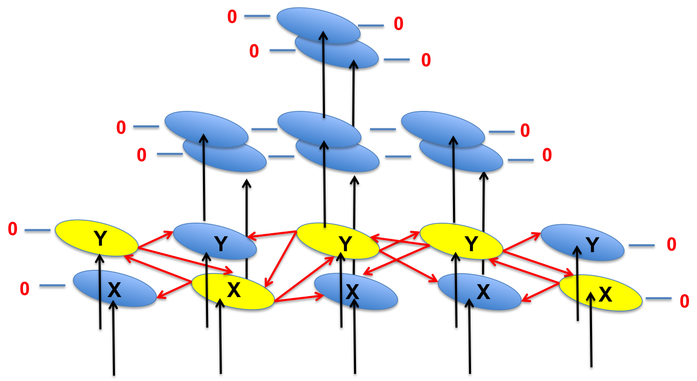
An input pattern is defined as a stimulus produced within the network. In Figure 1, each GN can analyse a symbol (“X” or “Y”) of a pattern comprising of five elements. In each GN (column) only the element with matching value (a row ID) would respond. For example, if the pattern is “YXYYX”, then in the second column “X” element will be activated as response to this input stimulus. If a particular element in the GN-column is activated it sends a report to all adjacent GNs. The report contains the activated GN’s element ID (the row index). Otherwise, it simply ignores the stimulus and returns to the idle state.
During the next phase, all GNs communicate the indices of the activated elements with the adjacent columns at their level, and additionally communicate the stored bias information to the layer above. The procedure continues in an ascending manner until the collective bias information reaches the top of the hierarchy. The higher level GNs can thus provide a more authoritative assessment of the input pattern. The accuracy of HGN was demonstrated to be comparable to the accuracy of Neural Network with back-propagation [2].
III-B Fundamentals of Vector Symbolic Architecture and Binary Spatter Codes
Vector Symbolic Architecture is an approach for encoding and operations on distributed representation of information. VSA has previously been used mainly in the area of cognitive computing for representing and reasoning upon semantically bound information [4, 15].
The fundamental difference between distributed and localist representations of data is as follows: in traditional (localist) computing architectures each bit and its position within a structure of bits are significant (for example, a field in a database has a predefined offset amongst other fields and a symbolic value has unique representation in ASCII codes); whereas in a distributed representation all entities are represented by binary random vectors of very high dimension. These representations are also called Binary Spatter Codes (BSC), though for the remainder of the article we use term HD-vector when referring to BSC codes, for reasons of brevity. High dimensionality refers to that fact that in HD-vectors, several thousand positions (of binary numbers) are used for representing a single entity; [4] proposes the use of vectors of 10000 binary elements. Such entities have the following useful properties:
III-B1 Randomness
Randomness means that the values on each position of an HD-vector are independent of each other, and "0" and "1" components are equally probable. In very high dimensions, the distances from any arbitrary chosen HD-vector to more than 99.99 % of all other vectors in the representation space are concentrated around 0.5 Hamming distance. Interested readers are referred to [4] and [16] for comprehensive analysis of probabilistic properties of the hyperdimensional representation space.
Denote the density of a randomly generated HD-vector (i.e. the number of ones in a HD-vector) as . The probability of picking a random vector of length with density , where the probability of 1’s appearance equals is described by described by the binomial distribution (1):
| (1) |
When is in the range of several thousand binary elements, the calculation of the binomial coefficient requires sophisticated computations. The following equations use an approximation of the binomial distribution, via the de Moivre-Laplace theorem:
| (2) |
III-B2 Similarity metric
A similarity between two binary representation is characterized by Hamming distance, which (for two vectors) measures the number of positions in which they differ:
,
where , are bits on positions in vectors and of dimension , and where denotes the bit-wise XOR operation.
III-B3 Generation of HD-vectors
Random binary vectors with the above properties can be generated with Zadoff-Chu sequences [17], a method widely used in telecommunications to generate pseudo-orthogonal preambles. Using this approach a sequence of vectors, which are pseudo-orthogonal to a given initial random HD-vector (i.e. Hamming distance between them approximately equals 0.5) are obtained by cyclically shifting by positions, where . Further in the article this operation is denoted as . The cyclic shift operation has the following properties:
-
•
it is invertible, i.e. if then ;
-
•
it is associative in the sense that ;
-
•
it preserves Hamming weight of the result:
; and -
•
the result is dissimilar to the vector being shifted:
.
Note that the cyclic shift is a special case of the permutation operation [4]. In the context of VSA, permutations were previously used to encode sequences of semantically bound elements.
III-B4 Bundling of vectors
Joining several entities into one structure is done by the bundling operation; it is implemented by a thresholded sum of the HD-vectors representing the entities. A bit-wise thresholded sum of vectors results in 0 when or more arguments are 0, and 1 otherwise. Furthermore terms "thresholded sum" and "majority sum" are used interchangeably and denoted as . The relevant properties of the majority sum are:
-
•
the result is a random vector, i.e. the number of ‘1’ components is approximately equal to the number of ‘0’ components;
-
•
the result is similar to all vectors included in the sum;
-
•
the number of vectors involved into MAJORITY sum must be odd;
-
•
the more HD-vectors that are involved in a majority operation, the closer the Hamming distance between the resultant vector and any HD-vector component is to 0.5; and
-
•
if several copies of any vector are included into a majority sum, the resultant vector is closer to the dominating vector than to other components.
The algebra on VSA includes other operations e.g., binding, permutation [4]. Since we do not use them in this article, we omit their definitions and properties.
IV Holographic Graph Neuron
This section presents one of the main contributions of this paper: the adoption of the VSA data representation for implementation of the HGN approach.
IV-A Motivation for Holographic Graph Neuron and outline of the solution
An important issue in hierarchical models is the overhead of resource requirements, specifically with regards to the number of processing elements required. We propose a holographic approach, which enables a flat GN array to operate with higher level of accuracy and comparable recall time than that of HGN, without the need for a complex topology and additional nodes. The high-level logic of the proposed solution is illustrated in Figure 2. Essentially, we replace the need for maintaining topological relationships by compacting parts of the pattern observed by GNs into one holographic representation.

IV-B Encoding
In the case of HoloGN, all its elements (i.e. symbols of individual neurons) are indexed uniquely and the index of a particular element is derived as a function of the GN’s ID. Let be an initialization high-dimensional vector for GN . The initialized vectors for different GNs are chosen to be mutually orthogonal. Then the HD-index of element in GN is computed as , where is a cyclic shift operation resulting in the generation of a vector orthogonal to HD-vector [17, 18].
IV-C Construction of VSA-representation of activated GNs
Let be the number of individual Graph Neurons. When a GN array is exposed to a pattern, the activated elements communicate their HD-represented indices to all other GNs; the holographic representation of the activated elements is then:
| (3) |
where is the HD-index of the activated element in , and the addition operation is the bundling operation, or thresholded sum as described in III-B. As discussed previously, in the resultant HD-vector the Hamming distances between each component and the composition vector is strictly less than 0.5. We will utilize this property later when constructing data structures for recall of patterns in HoloGN.
IV-D Data structures for storing and retrieving holographic representations in HGN elements
HoloGN will store the holographic representation of the entire pattern (3) observed across all GNs. A possible architecture is for all memorized patterns to be collected and stored centrally at a processing node.
Depending on the particular application of HoloGN, the memorized patterns could be stored either in an unsorted list or in bundles. The first mode of storing HoloGN patterns corresponds to the case where the structure of the observed patterns is unknown; the latter mode is used in the case of a supervised learning. The next section describes different HoloGN usage and recall strategies.
V HoloGN recall strategies
This section introduces and evaluates the performance of two major recall modes: the one-shot case and the case of supervised learning.
V-A Time-efficient -accurate recall in an unsorted HoloGN storage
The common steps in both recall modes is the procedure for the time-efficient search over an (unsorted) list of HoloGN records. Recall that all manipulations with VSA-encoded entities are done using simple bit-wise arithmetic operations as well, and calculations to obtain the Hamming distance between entities. However, for this article we assume no particular optimized implementation of VSA’s bit-wise operations; this is because such operations are tailored to the architectures of specific microprocessors, which operate with words of substantially lower dimensionalities (typically 32 or 64 bits). Therefore, adopting these methods for implementing the bit-wise operations on words of thousands of bits would be cumbersome. Instead, an easily analyzable computational model is adopted in this article, which could also be adapted to an implementation on specialized computing architectures.
In what follows, each HoloGN pattern is modelled as a row vector of elements. The list of stored HoloGN patterns is therefore modelled as an matrix, where is the number of the learned (stored) HoloGN patterns. Denote this matrix as H. The task of recalling a pattern with a target accuracy of () is formulated as finding the rows in H with Hamming distance to the query pattern less than or equal to .
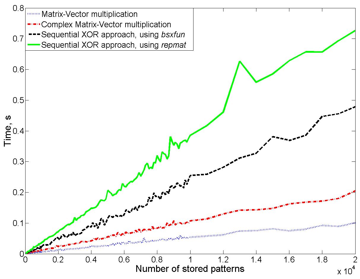
The conventional way of computing Hamming distance between vectors would be to perform the following sequence of computations for each row in H: 1) perform an element-wise XOR with the vector query; 2) sum up all elements in the intermediate result; and then 3) divide the result by the dimensionality of the vectors. The performance of the two implementations of this method using Matlab’s and functions are shown by the top two curves in Figure 3. The curves demonstrate linear but rapid increase in the recall time with the increase in the number of the stored patterns. The lowest curve in the figure shows the performance of matrix-vector multiplication of the same size, which is chosen as the reference case. The results were obtained on a Intel Core i7-3520M 2.9 GHz machine with Windows 7 operating system using one processor.
V-A1 Binary spatter codes as complex numbers
In order to improve the efficiency of calculating Hamming distances over a vast number of HoloGN patterns, we propose representing HoloGN patterns using complex numbers, where a binary would be represented by (i.e. the complex number) and a binary would remain . The intuition behind this transformation is simple: multiplication of bits in the same position should produce three outcomes: , and . That is, the multiplication of two similar bits would produce a real number and the multiplication of two different bits produces a imaginary number. In this way the sum of the imaginary parts over all positions in the resulting vector, divided by dimensionality , will correspond to the Hamming distance between the two vectors. Thus, the suggested method allows us to implement the calculation of Hamming distance through the standard method of matrix-vector multiplication, as illustrated below:
| (4) |
The performance of the proposed method is illustrated by the red dashed curve in Figure 3. It demonstrates that the calculation of the Hamming distance is only two times slower than the usual matrix-vector multiplication. Specifically, to compute Hamming distance from the target vector to each of 20 000 stored patterns takes approximately 200 ms on the test machine. Further optimization of the matrix multiplication and execution on parallel architectures hint on realistic bounds on the recall time over extremely large numbers of patterns.
V-B Case-study 1: Best-match probing under one-shot learning
The first usage of HoloGN is probing the existence of the target query pattern amongst the previously memorized patterns. The perfect match in this case would be indicated by a Hamming distance of zero. The deviation from zero, therefore, reflects the degree of proximity of the query to one or several stored HoloGN patterns. In the following example the accuracy of the HoloGN recall was compared to the performance of the original HGN approach. For the sake of fair comparison the 7 by 5 pixels letters of the Roman alphabet (as in [2]) were used.
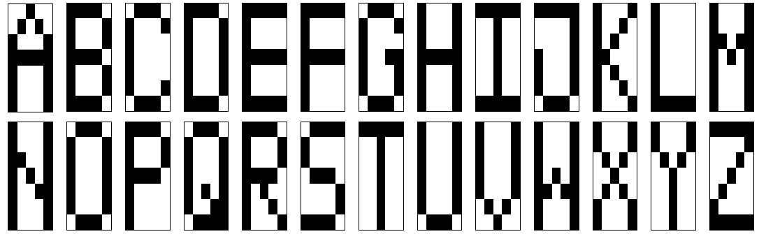
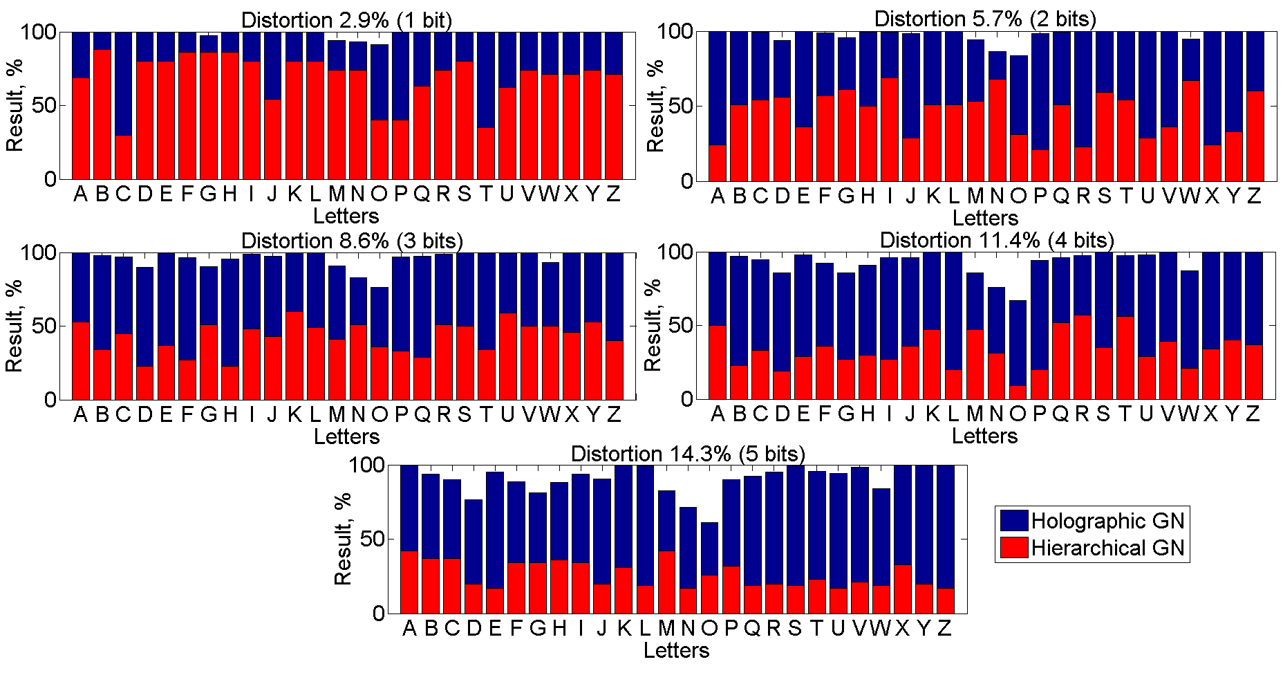
In the memorizing phase a set of noise-free images of letters illustrated in Figure 4 was presented to both architectures. In the recall phase images of the same letters distorted with different levels of random distortions (between 1 bit corresponding to a distortion of 2.9% of the pattern’s size and 5 bits equivalent to 14.3% distortion) were presented to the architectures for the recall. An example of a noisy input is presented in Figure 5. In the case of HoloGN the pattern with the lowest Hamming distance to the presented distorted pattern was returned as the output.
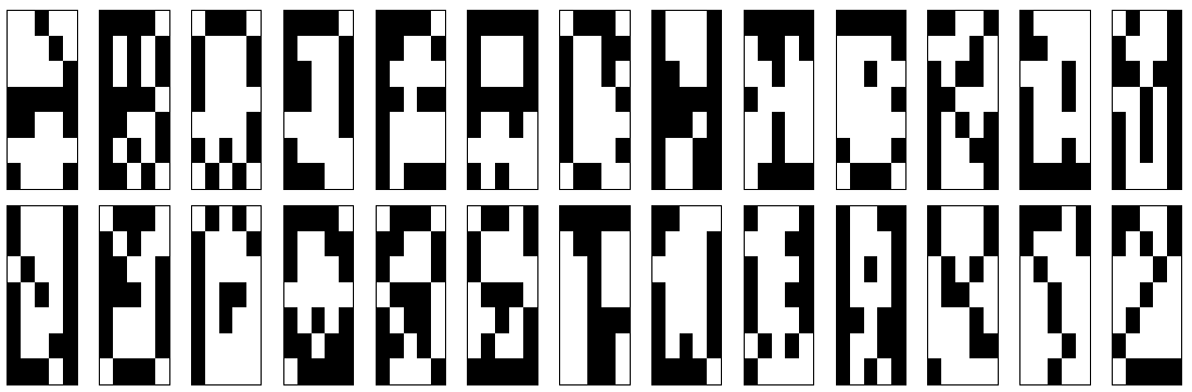
Figure 6 presents the results of the accuracy comparison between the recall results for the HoloGN approach and the reference HGN architecture. To obtain the results 1000 distorted images of each letter for every level of distortion were presented for recall. The charts show the percentage of the correct recall output. The analysis shows that the performance of the HoloGN-based associative memory at least matches that of the original approach. In most of cases HoloGN appears to be more accurate when recalling patterns with high level of distortion.
V-C Case-study 2: HoloGN recall under the supervised learning
The analysis presented above is a very positive result for the proposed bio-inspired associative memory based pattern processing architecture, since the accuracy of the original HGN approach was demonstrated to be as accurate as artificial neural networks with back-propagation [2]. While establishing formal relationships to the framework of artificial neural networksis outside the scope of this work, this section presents the results of the pattern recognition accuracy of the HoloGN architecture under the supervised learning. In this case the HoloGN is presented with a series of randomly distorted patterns for each letter with different level of distortion (between 3% and 43%) as exemplified in Figure 5. In the experiments up to 500 patterns for each letter and every level of distortion were presented for memorizing. For the particular level of distortion all presented patterns of the particular letter were bundled to a single HoloGN representation as
| (5) |
Thus by the end of the learning phase the HoloGN list will contain 26 high dimensional bundles, each jointly representing all (presented) distorted variants of the particular letter. In the recall phase for each distortion level HoloGN was presented with 500 new distorted patterns of each letter. The accuracy of the recall was measured as the percentage of the correctly recognized letters averaged over the alphabet.
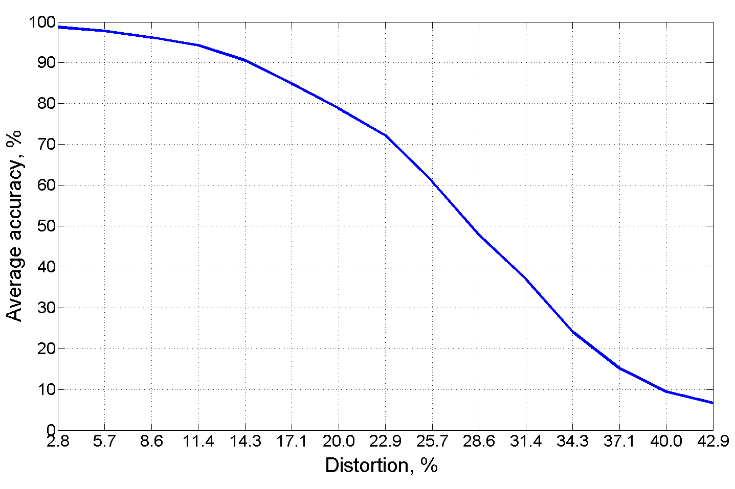
Figure 7 illustrates the obtained results: 90% accurate recall was observed when learning symbols distorted up to 15%. While the accuracy predictably decreases rapidly with the increase of distortion in the presented patterns, a reasonable 80% recall accuracy was observed for learning sets with 7 bits distortion (20%).
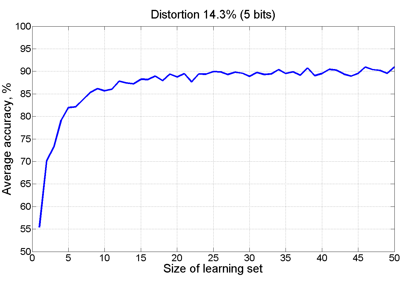
Figure 8 illustrates the convergence of the HoloGN recall accuracy with the number of presented noisy samples for the case of 14.3% distortion (5 bits). This is a definitely positive result for the presented architecture, which illustrates the suitability of the HoloGN in applications requiring supervised learning.
VI Pattern decoding and subpattern-based analysis
There is a class of pattern recognition applications which requires an understanding of the details of the recall results. For example, when a recall returns several possible patterns of given recall accuracy, the task would be to understand the overlapping elements. This section considers two aspects of this task: a robust decoding of elementary components out of a distributed VSA representation; and a quantitative metric of the similarity via direct comparison of distributed representations, without the need for decoding those representations.
The VSA approach of representing data structures by definition makes decoding of the individual components a tedious task, requiring a brute force test on the inclusion of all possible high-dimensional codewords for each GN. The majority sum, which is used for creating HoloGN representations of the observed patterns imposes a limit on the number high-dimensional codewords operands, above which a robust decoding of the individual operands is impossible.
VI-A Preliminaries
Denote the density of a randomly generated HD-vector (i.e. the number of ones in a HD-vector) as . The probability of picking a random vector of length with density , where the probability of 1’s appearance, defined as , is described by (2). The mean density of a random vector is equal to . Note that in reality the density of randomly generated HD-vectors will obviously deviate from the mean value. However, according to (1) density is approaches the mean value with the increase of dimensionality . In other, words the probability of generating HD-vector with or decreases with the increase of dimensionality .
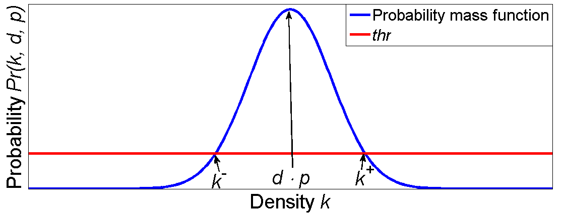
Define as the threshold probability of generating a vector with a certain deviation of density being negligibly small. Let and characterize the lower and the upper bounds of the interval of possible densities. This is illustrated in Figure 9. The bounds for a given , and are calculated using (2). The bounds are calculated according to (6) and (7). The value of threshold is chosen to be small ().
| (6) |
| (7) |
VI-B Capacity of HoloGN representations
Suppose there exists an item memory [4] containing HD-vectors representing atomic concepts333In the case of HoloGN an atomic concept is the code for the particular HoloGN element.. Recall that when several HD-vectors are bundled by the majority sum the noise of flipped bits increases with the number of components. For a given dimensionality there is a limit on the number of bundled HD-vectors beyond which the resulting HD-vector becomes orthogonal to every component vector; hence the A capacity of the resulting vector is defined as the maximal number of mutually orthogonal HD-vectors which can be robustly decoded from their majority sum composition by probing the item memory.
In order to characterize the capacity of the composition vector for a given dimensionality, one needs to characterize the level of noise introduced by the bundling operation. This is calculated as in [19] by (8), where is a number of atomic vectors in the resulting majority sum vector.
| (8) |
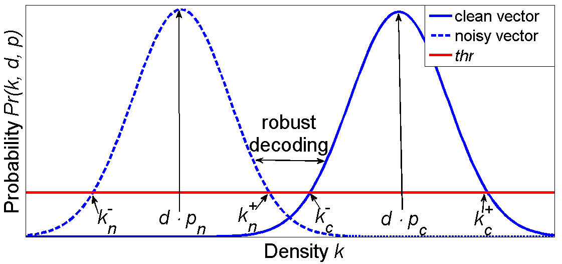
Consider an arbitrary HD-vector A to be decoded from a majority sum composition. Let N be a vector of noise imposed by the majority sum operation. Since the components are mutually orthogonal, the density of ones in the noise vector is also described the binomial distribution . As each new vector is added the level of noise increases, hence the mean of the noise vector density will approach 0.5 as illustrated in Figure 11. Due to the properties of high dimensional space, vector A will be undecodable when the upper bound of the density of noise vector N approaches the lower bound . That is, the noisy version of A becomes orthogonal to its clean version. This logic is illustrated in Figure 10, where the resulting majority sum vector is orthogonal to all components. Thus the capacity of the distributed representation with dimensionality is computed by:
| (9) |
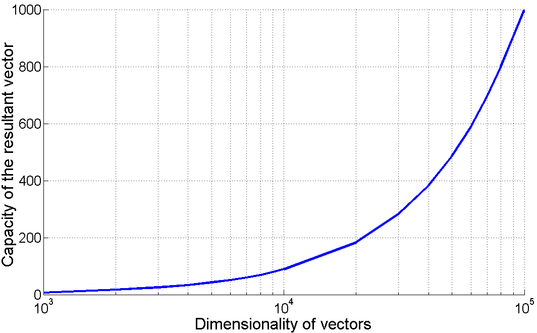
Figure 11 presents the capacity of HD-vector of different dimensionalities calculated for threshold probability . Specifically for bits the capacity of the robustly decodable VSA is 89 vectors.
VI-C Calculation of the number of common component vectors in two resulting vectors
Given the rather conservative limits on the number of robustly decodable elements in a distributed representation it is important that the proposed HoloGN architecture can estimate the similarity between different patterns without decoding them. This subsection provides a method for the quantitatively measuring the number of overlapping elements as a function of their relative Hamming distance. Denote and as lengths of two patterns, , and denote as the number of common elements in these patterns. Let M be a matrix of common elements where each row contains a random HD-vector of dimension encoding element . Denote an arbitrary column of matrix M as C. Since rows in M are independent, the density of ones in each column also follows the binomial distribution with and length . Denote the number of ones in column C as .
In order to calculate the Hamming distance between the distributed representations of two patterns with known , and , consider all possible cases when bits in the same position are different. The Hamming distance between two patterns can be estimated with equation (10):
| (10) |
where stands for the probability of having (0 or 1), when the representation consists of or atomic vectors and of these vectors are overlapped.
Due to the symmetry in the calculation of probabilities, is presented only for the case of . There are three possible cases for calculation of :
-
•
if is more than , then the result of the majority sum is ‘1’, i.e. is 1;
-
•
if number of possible ‘1’s is less than , then probability of is 0;
-
•
otherwise the probability should take into account all possible combinations, and their probabilities.
| (11) |
| (12) |
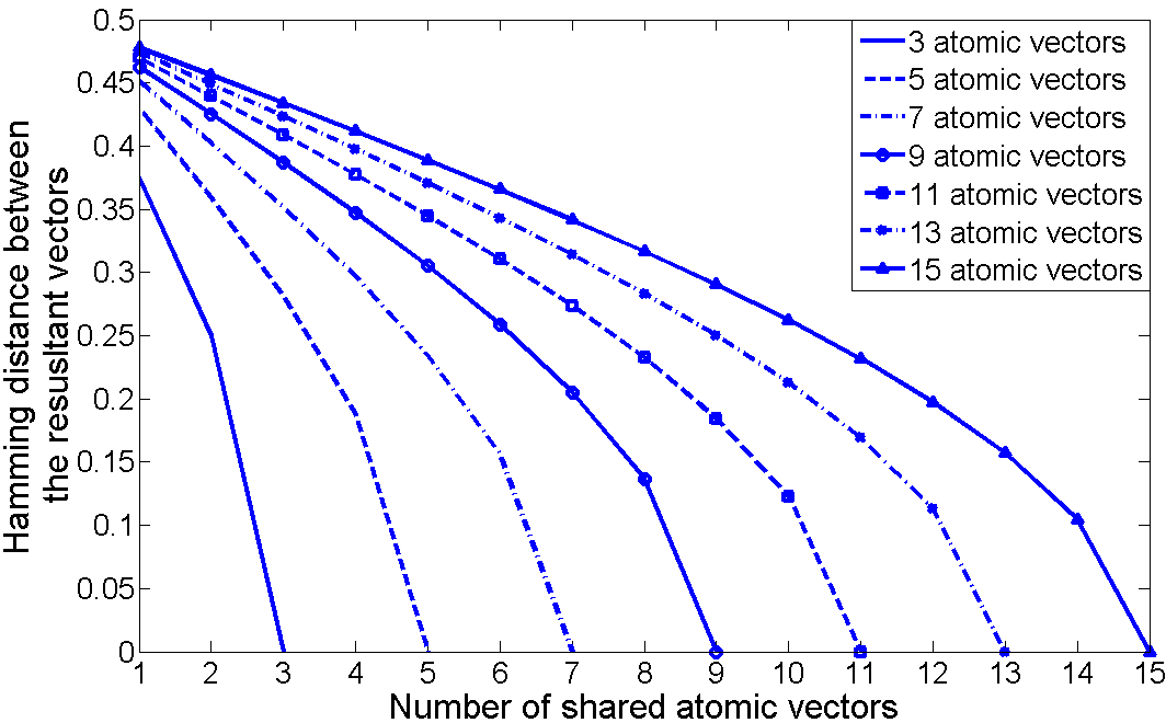
Figure 12 shows the Hamming distances between two resulting vectors for different numbers of overlapping vectors. The results show that the larger the number of common elements, the smaller the Hamming distance between resulting vectors.
This method opens a way towards constructing and analyzing patterns far beyond VSA’s robustly decodable capacity. The problem with practical application of this method, however, comes with the rapid convergence of the Hamming distance indicator to 0.5, making the difference between analyzable patterns indistinguishable as illustrated in Figure 12. For example, for HoloGN representations of patterns with 15 elements, sub-patterns of 3 overlapped elements are robustly detected, while patterns with fewer overlapped elements are indistinguishable. Thus, the minimal number of overlapped elements in two patterns which can be robustly detected using the Hamming distance indicator is called bundle’s sensitivity.
The analysis of the sensitivity is similar to the analysis of the capacity of VSA representation in section VI-B. For two patterns of length and elements, and overlapped components, the sensitivity is calculated by (13):
| (13) |
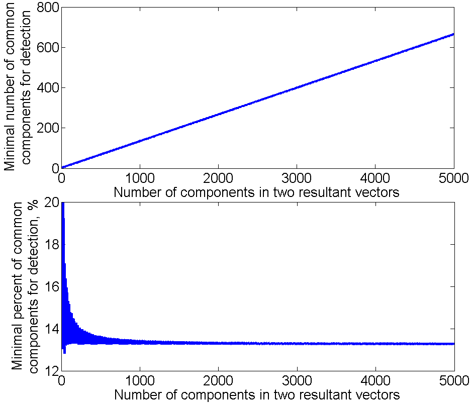
Figure 13 demonstrates the development of the sensitivity threshold with the number of elements in the compared patterns. The results show that the number of components for robust detection grows linearly with the size of pattern. Patterns with more than 500 elements should contain at least 14 % overlapped elements to be robustly detected by the proposed method.
VII Conclusion
This article presented Holographic Graph Neuron - a novel approach for memorizing patterns of generic sensor stimuli. HoloGN is built upon the previous Graph Neuron algorithm and adopts a Vector Symbolic representation for encoding of the Graph Neuron’s states. The adoption of the Vector Symbolic representation ensures a one-layered design for the approach, which implies the computational simplicity of the operations. The presented approach possesses the number of uniques properties. Prior to all, it enables a linear (with respect to the number of stored entries) time search for an arbitrary sub-pattern. While maintaining the previously reported properties of Hierarchical Graph Neuron, HoloGN is also improving the noise resistance of the architecture by this substantially improving the accuracy of pattern recall.
References
- [1] E. Osipov, A. I. Khan, and A. Anang. Holographic graph neuron. In Computer and Information Sciences (ICCOINS), 2014 International Conference on, pages 1–6. IEEE, 2014.
- [2] B. B. Nasution and A. I. Khan. A hierarchical graph neuron scheme for real-time pattern recognition. IEEE Transactions on Neural Networks, 19(2):212–229, February 2008.
- [3] A.I. Khan and A.H. Muhamad Amin. One-shot associative memory method for distorted pattern recognition. In AI 2007: Advances in Artificial Intelligence, 20th Australian Joint Conference on Artificial Intelligence, Gold Coast, Australia, volume 4830, pages 705–709, 2007.
- [4] P. Kanerva. Hyperdimensional computing: An introduction to computing in distributed representation with high-dimensional random vectors. Cognitive Computation, Springer, 1(2):139–159, October 2009.
- [5] S.D. Levy and R. Gayler. Vector symbolic architectures: A new building material for artificial general intelligence. In Proceedings of the 2008 Conference on Artificial General Intelligence 2008: Proceedings of the First AGI Conference, pages 414–418, Amsterdam, The Netherlands, The Netherlands, 2008. IOS Press.
- [6] T. Plate. Holographic reduced representations. IEEE Transactions on Neural Networks, 6(3):623–641, 1995.
- [7] S. I. Gallant and T. W. Okaywe. Representing objects, relations, and sequences. Neural Computation, 25(8):2038–2078, 2013.
- [8] R. Zbikowski. Fly like a fly. IEEE Spectrum, 42(11):46–51, November 2005.
- [9] Y. M. Song, Y. Xie, V. Malyarchuk, J. Xiao, I. Jung, K-J. Choi, Z. Liu, H. Park, C. Lu, R-H. Kim, R. Li, K. B. Crozier, Y. Huang, and J. A. Rogers. Digital cameras with designs inspired by the arthropod eye. Nature, 497(7447):95–99, May 2013.
- [10] K. J. Schultz. Content Addressable Memory. N. T. Limited, 1999.
- [11] P. Kanerva. A family of binary spatter codes. In ICANN ’95: International Conference on Artificial Neural Networks, pages 517–522, 1995.
- [12] S. Bajracharya S. Levy and R. Gayler. Learning behavior hierarchies via high-dimensional sensor projection. 2013.
- [13] D. Kleyko, N. Lyamin, E. Osipov, and L. Riliskis. Dependable mac layer architecture based on holographic data representation using hyper-dimensional binary spatter codes. In Multiple Access Communications : 5th International Workshop, MACOM 2012, pages 134–145. Springer, 2012.
- [14] P. Jakimovski, H.R. Schmidtke, S. Sigg, L. Weiss-Ferreira-Chaves, and M. Beigl. Collective communication for dense sensing environments. Journal of Ambient Intelligence and Smart Environments (JAISE), 4(2):123–134, March 2012.
- [15] T. Plate. Distributed Representations and Nested Compositional Structure. University of Toronto, PhD Thesis, 1994.
- [16] P. Kanerva. Sparse distributed memory. The MIT Press, 1988.
- [17] B.M. Popovic. Generalized chirp-like polyphase sequences with optimum correlation properties. Information Theory, IEEE Transactions on, 38(4):1406–1409, 1992.
- [18] D. Kleyko and E. Osipov. On bidirectional transitions between localist and distributed representations: The case of common substrings search using vector symbolic architecture. Procedia Computer Science, pages 1–10, 2014.
- [19] P. Kanerva. Fully distributed representation. In Real world computing symposium, pages 358–365, 1997.