Theoretical study of radiative electron attachment to CN, C₂H, and C₄H radicals

Abstract

A first-principle theoretical approach to study the process of radiative electron attachment is developed and applied to the negative molecular ions CN^-, C₄H^-, and C₂H^-. Among these anions, the first two have already been observed in the interstellar space. Cross sections and rate coefficients for formation of these ions by radiative electron attachment to the corresponding neutral radicals are calculated. For completeness of the theoretical approach, two pathways for the process have been considered: (i) A direct pathway, in which the electron in collision with the molecule spontaneously emits a photon and forms a negative ion in one of the lowest vibrational levels, and (ii) an indirect, or two-step pathway, in which the electron is initially captured through non-Born-Oppenheimer coupling into a vibrationally resonant excited state of the anion, which then stabilizes by radiative decay. We develop a general model to describe the second pathway and show that its contribution to the formation of cosmic anions is small in comparison to the direct mechanism. The obtained rate coefficients at 30 K are $7\times 10^{-16}$cm³/s for CN^-, $7\times 10^{-17}$cm³/s for C₂H^-, and $2\times 10^{-16}$cm³/s for C₄H^-. These rates weakly depend on temperature between 10K and 100 K. The validity of our calculations is verified by comparing the present theoretical results with data from recent photodetachment experiments.

I Introduction

The present theoretical study of radiative electron attachment (REA) to neutral molecules is motivated by the recent discoveries of molecular anions in the interstellar medium (ISM). Six anions have been detected so far in the ISM: C₆H^- McCarthy et al. (2006); Cernicharo et al. (2007); Herbst and Osamura (2008); Harada and Herbst (2008); Cernicharo et al. (2008), C₄H^- H. Gupta and S. Brünken and F. Tamassia and C. A. Gottlieb and M. C. McCarthy and P. Thaddeus (2007), C₈H^- Kawaguchi et al. (2007), C₃N^- Thaddeus et al. (2008), C₅N^- Cernicharo et al. (2007, 2008), and CN^- Agúndez et al. (2010). The possibility for atomic anions, such as H^-, to be formed in the ISM by REA was first suggested by McDowell McDowell (1961) in 1961. Later, Dalgarno and McCray Dalgarno and McCray (1973) have discussed the role of negative atomic ions in the formation of neutral molecules in the ISM. The formation of molecular anions in the ISM by REA has been proposed by Herbst Herbst (1981), who has also developed a theoretical approach Herbst (1981); Herbst and Osamura (2008) to evaluate rate coefficients for REA. More than twenty years after his prediction, negative molecular ions were indeed detected in the ISM.

The theoretical approach proposed by Herbst, the phase-space theory (PST), has been used in a number of studies Herbst (1981); Herbst and Osamura (2008); Herbst (1985); R. Terzieva and E. Herbst (2000); Petrie and Herbst (1997); Millar et al. (2007); Petrie (1996) to calculate the REA rate coefficients and to model formation of anions in the ISM. The approach has been successful in interpreting the observed column density of C₈H^-, C₆H^-, C₅N^- and C₃N^- ions, while the agreement with observations is not as good for the C₄H^- and CN^- ions.

PST relies on several assumptions. First, it considers REA as a two-step process, schematically represented in Fig. 1 for the case of CN/CN^-. As a first step, the incident electron is captured by a neutral target molecule $M$ into an electronic state of $M^{-}$ through non-Born-Oppenheimer coupling, thus forming a vibrational resonance of $M^{-}$ in a highly-excited vibrational level. The resonance can decay back to the $M+e^{-}$ electronic continuum spectrum through the same non-Born-Oppenheimer coupling, i.e. the electron can autodetach. Another possibility for the resonance, considered as the second PST step, is to emit a photon, thus stabilizing the $M^{-}$ system. In PST, it is assumed that the probability of the first step of the process is unity and, therefore, the cross section for the electron capture is approximated by the unitary limit formula for $s$-wave scattering Herbst and Osamura (2008) $\sigma_{c}=\pi/k^{2}$, where $k$ is the wave number of the incident electron with energy $E_{el}=(\hbar k)^{2}/(2m_{e})$, and $m_{e}$ is the electron mass. In the second PST step, stabilization of the $M^{-}$ resonance is represented as an emission of a photon by a set of harmonic oscillators of the molecule in the normal mode approximation of molecular vibrations. A larger number of available vibrational modes decreases the probability of autodetachment, and thus allows for a larger probability in the second PST step. Therefore, in PST, the overall two-step REA cross section $\sigma_{PST}$ grows rapidly with the number of atoms in the molecule and approaches the unitary limit $\sigma_{PST}\to\sigma_{c}$. For example, the REA rate coefficient for formation of CN^- calculated by PST is about $10^{-17}$cm³/s Petrie (1996) and much larger, $3\times 10^{-7}$cm³/s, for C₆H^- Herbst and Osamura (2008) at 10K. For CN^- the theoretical value is smaller by several orders of magnitude than the one needed to explain the [CN^-]/[CN] abundance ratio obtained from the astrophysical observations.

The PST assumption about the unitary probability of the first step of the process can hardly be justified for small molecular ions. But it is possible to apply a quantum-mechanical approach based on first principles for the both steps of the REA mechanism, suggested by Herbst. Considering the process quantum-mechanically, another mechanism for REA is also possible: The electron incident on a neutral molecule emits a photon and becomes bound without an intermediate step of capture into a vibrationally excited state of the ground electronic state of the negative ion. To distinguish the two mechanisms, we call the first one as indirect (IREA) and the second mechanism as direct REA (DREA). The total cross section of the REA is the sum of DREA and IREA cross sections.

Recently, we have developed a fully-quantum theoretical approach for DREA based on first principles only Douguet et al. (2013). The approach considers the radiative electron attachment of a continuum electron through spontaneous decay to the anion ground state (see Fig. 1) and does not include an intermediate vibronic state of $M^{-}$ populated through the non-Born-Oppenheimer coupling, as represented by the two-step REA mechanism in PST. Hence, the approach relies on wave functions of the continuum spectrum of the $M+e^{-}$ system and transition dipole moments to the bound electronic state of $M^{-}$, calculated ab initio. Using the developed approach, we have calculated the REA cross section and rate coefficient for the formation of the cyanide ion, CN^-. Our results confirmed the previous assessment that the REA rate coefficient for CN^- is too small, $8\times 10^{-16}$cm³/s at 10 K Douguet et al. (2013), to explain the CN^- abundance observed in the ISM.

In the present study, we extend the theoretical approach to larger molecules. In order to assess the approximations employed in the PST approach, we also develop a quantum mechanical approach for IREA. In this study, we calculate explicitly the probability of electron capture during the first step of IREA process using ab initio methods and determine the overall cross section of the IREA process, which might be compared with the PST results.

Although there is no experimental data on the REA process for carbon chain molecules, using a similar theoretical approach, we determine in this study cross sections for the inverse process to REA, namely photodetachment (PD), and compare with available data from recent photodetachment experiments Kumar et al. (2013); Best et al. (2011). This allows us to verify the validity of our results.

In the next section, we present our theoretical approach to study DREA and apply it to the CN^-, C₂H^-, and C₄H^- ions. Section III is devoted to the comparison of the results obtained in this study with data from photodetachment experiments. Section IV presents the theoretical approach of IREA for the case of CN^-. In the Section V, we develop a model of IREA for larger molecules and we compare its results with those of PST. Finally, Section VI summarizes the important findings of the study.

II Direct mechanism of radiative electron attachment to CN, C₂H, and C₄H

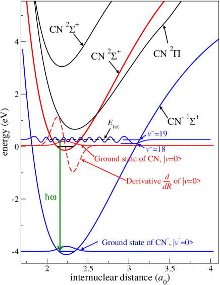
Figure 1: Schematic representation of two mechanisms for REA of an electron to the CN radical: (i) DREA: The electron incident on CN in its ground vibronic state spontaneously emits a photon of energy $\hbar\omega$ (green arrow) and forms the CN^- ground state. The photon energy is equal to the difference between the initial total energy of the system $E_{tot}$ (horizontal dashed line at near energy of the $v^{-}=19$ state) and the energy of CN^- ground state. (ii) IREA: As a first step of the process, the incident electron is captured via non-Born-Oppenheimer coupling into the ground electronic state of CN^- without emitting a photon. Because the total energy $E_{tot}$ is conserved, the vibrational level $v^{-}$ of CN^- in this first step of the process is highly excited: For low incident energies of the electron, it corresponds to $v^{-}=18$ or 19. After the first step, the electron captured in an excited vibrational level can either autodetach or stabilize by photon emission. The photon changes the rotational and vibrational states of the CN^- molecule. The largest probability for the second step corresponds to a change of $v^{-}$ by one quantum. The dashed red line shows the derivative of the vibrational ground state wave function of CN, which enters in the calculation of the non-Born-Oppenheimer coupling in Eq. (11).

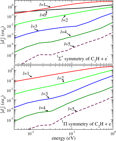
Figure 2: Matrix elements of the $d_{x}$ and $d_{z}$ components of the transition dipole moment between the C₂H^- electronic ground state and the $e^{-}+$C₂H system for several partial waves as a function of the incident electron energy, calculated at the equilibrium geometry of C₂H^-.

The cross section for DREA of an electron to a neutral linear molecule $M$, such as C_nH ($n=2,4$) or C_mN ($m=1,3$), initially in its electronic ground state with the vibrational level $v$ and energy $E_{i}$, was given in Douguet et al. (2013) and is expressed as

$$\sigma_{i}=\frac{4}{3}\frac{\pi\omega^{3}m_{e}}{k^{2}\hbar^{2}c^{3}}\sum_{l\pi}\left|d_{\pi,\Gamma l-\pi}^{(v\to v_{f})}\right|^{2}\,,$$ (1)

where $v_{f}$ is the vibrational state of the ion $M^{-}$ with total energy $E_{f}$ formed after DREA; $\omega$ is the frequency of the emitted photon, $\hbar\omega=E_{i}+E_{el}-E_{f}$. The quantities $d_{\pi,\Gamma l\lambda}^{(v\to v_{f})}$ are matrix elements of the components $\pi=-1,0,+1$ of the dipole moment operator between the initial $\Psi_{\Gamma l\lambda}$ ($M$+incident electron) and the final $\Psi_{f}$ electronic state, integrated over the initial $\chi_{v}(\vec{q})$ and final $\chi_{v_{f}}(\vec{q})$ vibrational wave functions of $M$ and $M^{-}$, respectively, and $\vec{q}$ denotes collectively all internuclear degrees of freedom. Their values are given by

$$d_{\pi,\Gamma l\lambda}^{(v\to v_{f})}=\int\chi_{v_{f}}(\vec{q})\langle\Psi_{f}|d_{\pi}|\Psi_{\Gamma l\lambda}\rangle\chi_{v}(\vec{q})d\vec{q}\,,$$ (2)

(see details in Ref. Douguet et al. (2013)); with $l$ the electronic partial wave angular momentum and $\lambda$ its projection on a specific axis in the molecular frame. The matrix elements $\langle\Psi_{f}\arrowvert d_{\pi}\arrowvert\Psi_{\Gamma l\lambda}\rangle$ of the dipole moment operator $\hat{d}_{\pi}$ are given by the integral

$$\langle\Psi_{f}\arrowvert d_{\pi}\arrowvert\Psi_{\Gamma l\lambda}\rangle = -\sum^{N}_{k=1}\int\Psi_{f}^{*}(r_{1},\cdots,r_{N})er_{k\pi}$$ (3)

$$\times\Psi_{\Gamma l\lambda}(r_{1},\cdots,r_{N})d^{3}r_{1}\cdots d^{3}r_{N},$$

where the function $\Psi_{f}$ represents the $N$-electron final state of the negative ion ($r_{1}$,…,$r_{N}$ are the coordinates of the electrons), $\Psi_{\Gamma l\lambda}$ is the electronic continuum state representing the scattering electron with $l$ and $\lambda$ angular quantum numbers, and $\Gamma$ labels the initial neutral electronic target state with $N-1$ electrons. Finally, $r_{k\pi}$ is one of the three cyclic components ($\pi=0,\pm 1$) of the coordinate of the $k^{\mathrm{th}}$ electron

$$r_{k\pi}=\left\{\begin{array}[]{l}z_{k},~{}{\rm if}~{}\pi=0\\ \mp(x_{k}\pm iy_{k})/\sqrt{2},~{}{\rm if}~{}\pi=\pm 1\,.\end{array}\right.$$ (4)

The calculations of the electronic wave functions and transition dipole moments (TDMs) of Eq. (3) are performed using the complex Kohn variational method, extensively described in past studies C. W. McCurdy and T. N. Rescigno (1989); Orel et al. (1991).

The DREA cross section for the formation of CN^-, starting from the ground vibrational level $v=0$ of CN, was calculated using Eq. (1) Douguet et al. (2013). The vibrational integral of Eq. (2) was computed explicitly from the geometry-dependent matrix elements $\langle\Psi_{f}|d_{\pi}|\Psi_{\Gamma l\lambda}\rangle$ obtained in the complex Kohn calculations. These matrix elements, as a function of the electron energy and of the internuclear distance, were respectively shown in Fig. 3 and Fig. 4 of Ref. Douguet et al. (2013).

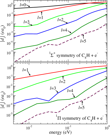
Figure 3: Same as Fig. 2 for the $e^{-}+$C₄H system.

The calculation of the TDMs is computationally intensive, especially for polyatomic molecules. In Ref. Douguet et al. (2013), we found that the TDMs weakly depend on the geometry of the molecule near its equilibrium position. Therefore, it seems reasonable to use the Franck-Condon approximation and simplify the calculation of the vibrational integral in Eq. (2) by using the value of $\langle\Psi_{f}|d_{\pi}|\Psi_{\Gamma l\lambda}\rangle$ at a fixed molecular geometry, e. g. the equilibrium position of the negative ion or the equilibrium of the neutral molecule, which are close to each other. The TDMs then take the simple form

$$d_{\pi,\Gamma l\lambda}^{(v\to v_{f})}\approx\langle\Psi_{f}|d_{\pi}|\Psi_{\Gamma l\lambda}\rangle_{{\cal Q}_{0}}\int\chi^{*}_{v_{f}}(\vec{q})\chi_{v}(\vec{q})d\vec{q}\,,$$ (5)

where the subscript ${\cal Q}_{0}$ refers to the equilibrium geometry of the negative ion. For molecules such as C_nH and C_mN, for which the potential energy surfaces of the initial electronic state of the target and the final state of the negative ion are quite similar in shape near the equilibrium positions of the ion and the neutral molecule Douguet et al. (2014), the Franck-Condon integral in Eq. (5) is the largest for transitions with $v_{f}=v$, for which its value is close to unity. For instance, the Franck-Condon integral in Eq. (5) is about 0.90 for C₂H/C₂H^- and 0.87 for C₄H/C₄H^- Douguet et al. (2014). For transitions to other vibrational levels, the integral is significantly smaller. Therefore, the DREA cross section is well approximated by

$$\sigma_{i}\approx\frac{4}{3}\frac{\pi\omega^{3}m_{e}}{k^{2}\hbar^{2}c^{3}}\sum_{l\pi}\left|\langle\Psi_{f}|d_{\pi}|\Psi_{\Gamma l\lambda}\rangle_{{\cal Q}_{0}}\right|^{2}\,,$$ (6)

where the transition dipole moment is evaluated at the energy of the $M+e^{-}$ system. The transition dipole moments strongly depend on energy, especially for non-zero partial waves, $l>0$. At low energies, their behavior is described quite well by the Wigner threshold law Wigner (1948). The energy dependence of $\left|\langle\Psi_{f}|d_{\pi}|\Psi_{\Gamma l\lambda}\rangle_{{\cal Q}_{0}}\right|$ for C₂H/C₂H^- and C₄H/C₄H^- is shown in Figs. 2 and 3.

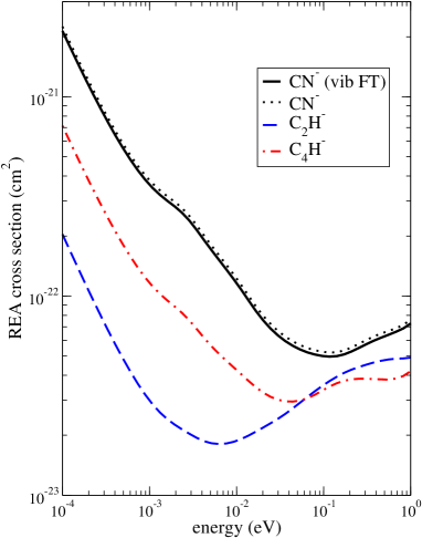
Figure 4: The cross sections for formation of CN^-, C₂H^-, and C₄H^- by DREA with the ground vibrational level $v=0$ of the neutral molecule as the initial state. The CN^- cross section is calculated in two different ways: The dotted line corresponds to the calculation using Eq. (6); the cross section shown with the solid line, ”vib FT” (vibrational frame transformation), is obtained evaluating the vibrational integral of Eq. (2) explicitly.

For C₂H and C₄H, the DREA cross sections were calculated using the approximate formula of Eq. (6), with the transition dipole moments determined only at the equilibrium geometry ${\cal Q}_{0}$ of the negative ion for several energies of the incident electron. For comparison, the DREA cross section for CN^- has been calculated using the direct integration over internuclear distances, Eqs. (1) and (2), as well as using Eq. (6). Figure 4 shows the DREA cross sections obtained for CN^-, C₂H^-, and C₄H^-. As can be seen in the figure, the CN^- cross sections obtained in the two ways are almost identical. Therefore, Eq. (6) gives a very good approximation of Eqs. (1) and (2) for CN^-. For C₂H/C₂H^- and C₄H/C₄H^- the approximation is likely less accurate because the vibrational functions of the neutral molecule and the ion are not as similar to each other as for CN^-.

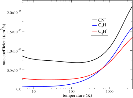
Figure 5: The REA thermally-averaged rate coefficients.

The obtained DREA cross sections have been used to determine the thermal rate coefficients, which are shown in Fig. 5. The rates for the formations of these three anions via DREA are too small to explain the astrophysical observations.

III Comparison with the results of photodetachment experiments

There is no experimental data on radiative electron attachment to the CN, C₂H, and C₄H molecules. However, the calculated transition dipole moments can be used to determine the photodetachment cross sections, for which experimental data on absolute values of photodetachment cross sections have recently been obtained for CN^- Kumar et al. (2013), C₂H^- Best et al. (2011) and C₄H^- Best et al. (2011) anions. Here, we discuss the interpretation of the photodetachment experiments only briefly. A detailed and more elaborated study can be found in Ref. Douguet et al. (2014).

The photodetachment cross section is given by (see, for example, Eq. (2.202) of Ref. Friedrich (2006))

$$\sigma_{PD}=\frac{4\pi^{2}\omega}{3c}\sum_{l\pi}\left|d_{l,\pi,E}\right|^{2}\,,$$ (7)

where $\omega$ is the photodetached photon frequency and $d_{l,\pi,E}$ is the dipole moment between the initial bound state and the final continuum state with energy $E$ and partial wave $l$ of the photodetached electron. The radial part of the wave function $\phi_{E}(r)$ of the initial electronic-continuum state used to calculate the transition dipole moment $d_{l,\pi,E}$ in Eq. (7) is energy-normalized. The continuum functions used in our calculation (see Eq. (3)) are normalized as

$$\phi_{E}(r)=\sqrt{\frac{2m_{e}}{\pi\hbar^{2}}}\Psi_{\Gamma l\lambda}\,.$$ (8)

Thus, the PD cross section can be written as

$$\sigma_{PD}=\frac{8m_{e}\pi\omega}{3\hbar^{2}c}\sum_{l\pi}\left|d_{\pi,\Gamma l-\pi}^{(v\to v_{f})}\right|^{2}\,.$$ (9)

For convenience of comparison with the results of the DREA calculations, the photon frequency can be expressed in terms of the electron affinity $E_{ea}$ and the energy $E_{el}$ of the incident (in DREA) or emitted (in PD) electron $\hbar\omega=E_{el}+E_{ea}$. This formula assumes that both initial and final vibrational levels are not excited, $v=v^{-}=0$, and that the zero-point energies for the neutral molecule and the ion are the same. The experimentally measured affinities are 3.862 eV for CN Bradforth et al. (1993), 2.969 eV for C₂H Ervin and Lineberger (1991); Zhou et al. (2007), and 3.558 eV for C₄H Taylor et al. (1998).

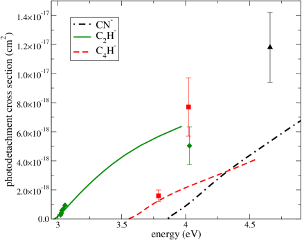
Figure 6: Theoretical (lines) and experimental (symbols with uncertainty bars) photodetachment cross sections for CN^-, C₂H^-, and C₄H^-. The triangle is the experimental result for CN^- Kumar et al. (2013), diamonds – C₂H^- Best et al. (2011) , squares – C₄H^- Best et al. (2011).

We discuss now the accuracy of the present calculations. The main source of uncertainty for the REA and PD cross sections for all three molecules considered here is the quality of electronic continuum and bound state wave functions. The quality of the electronic bound state wave function could be assessed in part by comparing the obtained theoretical affinity with the experimental one. The affinities corresponding to wave functions used in the present calculations, are 3.8 eV, 2.2 eV, and 3.0 eV for CN^-, C₂H^-, and C₄H^- respectively. Therefore, the agreement is about 1% for CN^- and much poorer, about 30%, for C₂H^- and C₄H^-. The quality of electronic continuum wave functions is more difficult to assess. Based on our previous experience with the electron-scattering calculations, we assume here that an additional uncertainty in the calculated transition dipole moments due to the quality of continuum wave functions is about 10% for CN^-, C₂H^-, and C₄H^-. These considerations give an estimated uncertainty in the REA and PD cross sections of about 20% for CN^- and 40% for C₂H^- and C₄H^-. For C₂H^- and C₄H^-, there are additional sources of uncertainty; the neglected geometry dependence of the transition dipole moments and the neglected role of rovibrational Feshbach resonances, which could be present at low collisional energies.

Figure 6 shows the PD cross sections calculated for CN^-, C₂H^-, and C₄H^- using Eq. (9) and compares them with the available experimental data, which were estimated in Ref. Best et al. (2011) to have about 25 % of uncertainty. The agreement is very good for C₂H^-, especially for experimental data points near the photodetachment threshold. The agreement for C₄H^- is also good for the lowest energy point, but is about a factor 2-3 lower than the experimental value for the second energy point. Similarly, the only experimental data point for CN^- measured at 4.65 eV gives a PD cross section twice larger than the theoretical value. The reason for this discrepancy is not clear. Overall, the agreement of the theoretical and experimental results is sufficient to conclude that the theory is reliable for calculations of photodetachment cross sections and, therefore, also for DREA cross sections. Thus, the results of photodetachment experiments validate the present theoretical approach for the DREA process and the results obtained using the approach. In particular, the present results and the PD experiments Kumar et al. (2013); Best et al. (2011) with C₄H^- and CN^- suggest that the observed abundance of these two ions in the ISM can hardly be explained by the DREA mechanism.

IV The contribution of the indirect process to the total REA cross section: The CN example

We now consider the process of radiative attachment mediated by the non-adiabatic couplings, through the IREA mechanism discussed in the introduction. In this section, we consider the IREA process for CN, for which the non-adiabatic couplings are evaluated numerically. We extend the approach to larger molecules in the next section.

The probability per unit time of a transition from the initial vibronic state $|i\rangle$ of the $e^{-}+$CN system described above into the final state of CN^- being in a vibrationally excited level $v_{f}\sim 19$ is given by the Fermi’s golden rule

$$P={\frac{2\pi}{\hbar}}\left|\langle f|\hat{\Lambda}|i\rangle\right|^{2}\rho(E_{c})\,,$$ (10)

where $\rho(E_{c})$ is the density of final states after the electron capture $\rho(E_{c})\sim 1/\Delta E_{rv}$, with $\Delta E_{rv}$ the energy splitting between rovibrational states, and $\hat{\Lambda}$ is the operator of non-adiabatic coupling. Denoting $R$ the CN internuclear distance, the matrix element $\Lambda_{fi}$ between initial and final vibronic states is

$$\Lambda_{fi}=\frac{\hbar^{2}}{\mu_{CN}}\int\chi^{*}_{v_{f}}(R)\Lambda_{f,\Gamma l\lambda}(R){\frac{\partial}{\partial R}}\chi_{v}(R)dR\,,$$ (11)

where $\mu_{CN}$ is the reduced mass of CN and $\Lambda_{f,\Gamma l\lambda}(R)$ is the following electronic matrix element

$$\Lambda_{f,\Gamma l\lambda}(R)=\int\Psi^{*}_{f}(\vec{r},R){\frac{\partial}{\partial R}}\Psi_{\Gamma l\lambda}(\vec{r},R)d\vec{r}\,.$$ (12)

In the above equation, $\vec{r}$ denotes collectively all electronic coordinates. Note that we neglected the second term of the non-adiabatic couplings, which is expressed with the second derivative of the electronic wave function with respect to the internuclear distance.

Calculating $\Lambda_{fi}$, we did not account for the integral over rotational coordinates. The latter integral is of the order of unity or smaller. A change of rotational quantum number $j$ during the process of the non-adiabatic electron attachment is unlikely for CN^- at low collision energies. This is because the values of the non-adiabatic couplings are the largest for $s$-wave scattering and much smaller for higher partial waves at low energies. Thus, we use the vibrational splitting in the formula for the density of states $\rho(E_{c})\sim 1/\Delta E_{v}$.

Numerical evaluation of the electronic matrix element $\Lambda_{f,\Gamma l\lambda}(R)$ of the non-adiabatic couplings was performed at several internuclear distances. Typically, non-adiabatic couplings can be calculated using standard ab initio programs, but such calculations are limited to couplings between electronic bound states, whereas in the present case, the initial electronic state belongs to the electronic continuum spectrum of the molecule. One possible way to calculate the couplings with a continuum state using standard ab initio programs is to include very diffuse orbitals in the bound-state calculations in order to cover the region of large electronic radial distance. As more diffuse functions are added to the basis set, a better description of the asymptotic region is achieved, which leads to the appearance of ”box-state” like wave functions with positive asymptotic energy. Such states resemble a scattering state of the electron if enough diffuse functions are added to the basis set. The box states should then be normalized appropriately to represent a continuum state. The latter approach should provide a reasonable approximation of the non-adiabatic couplings because no strong boundary conditions are imposed on the wave function. Performing numerical calculations, we have verified convergence of results (the non-adiabatic couplings) with respect to the number of added diffuse functions.

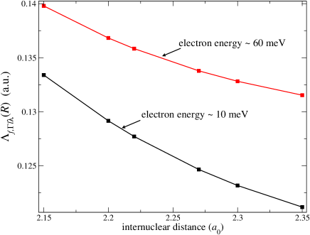
Figure 7: The matrix element of the non-adiabatic coupling operator of Eq. (12) evaluated for two different electronic ”quasi-continuum” states with energies $\sim$10 and $\sim$60 meV above the electronic threshold. The continuum state of the incident electron is normalized in the same way as in Ref. Douguet et al. (2013), where the current density of electrons in the incident plane wave is equal to the electron velocity (see Eqs. (10), (A2), and (A19) in Douguet et al. (2013)).

Since the calculations are performed in a finite volume represented by the space spanned by our diffuse basis set, the calculated electronic states of ${\rm CN}+e^{-}$ just above the CN threshold energy appear as a ”quasi-continuum” of states $\Psi^{l}_{n}$ with discretized energies. These states are labeled (in order of increasing energy above the electronic threshold) with index $n$ and with the dominant angular momentum $l$. The states should be rescaled to be energy normalized by multiplying by a factor $\Delta E^{-1/2}_{el}$, where $\Delta E_{el}$ is the energy difference between ”quasi-continuum” states. Because $\Delta E_{el}$ is changing from one state to another, it is taken here as the average between two energy differences for three neighboring ”quasi-continuum” states. The calculated values of $\Lambda_{f,\Gamma l\lambda}(R)$ are plotted in Fig. 7 for two ”quasi-continuum” $s$-wave scattering states. These states, corresponding to $n=2$ and $3$, and have respectively $\sim$10 and $\sim$60 meV asymptotic electron energy above the electronic threshold. Notice that the non-adiabatic couplings for the two states are similar and decrease with the internuclear distance. Furthermore, states with higher energies have larger couplings, which is expected from the Wigner threshold law because such couplings should increase approximately as $\sqrt{E_{el}}$. Because the low-energy non-adiabatic couplings associated with $p$-wave scattering states increase only as $E_{el}^{3/2}$, their values at low energy were found to be negligible in comparison with the couplings from $s$-waves scattering states. Finally, although the non-adiabatic couplings were obtained from an approximative treatment, their values should represent an estimation accurate enough for the purpose of this study.

The electron capture cross section is then obtained by dividing the probability by the current density $j_{cd}$ in the incident wave. If the incident wave is normalized as in Eqs. (A2) and (A19) of Ref. Douguet et al. (2013), the current density is then simply equal to the velocity of the incident electron $j_{cd}=v_{cd}$. It gives the following estimation for the cross section

$$\sigma_{c} = \frac{P}{j_{cd}}\approx\frac{\pi}{E_{el}}\frac{1}{\Delta E_{v}}\frac{\hbar^{4}}{\mu_{CN}^{2}}$$ (13)

$$\times\left|\int\chi_{v_{f}}^{*}(R)\Lambda_{f,\Gamma l\lambda}(R){\frac{\partial}{\partial R}}\chi_{v}(R)dR\right|^{2}\,.$$

In the above equation, we assumed that the ratio of the number of final rotational levels of the formed anion CN^- to the number of initial rotational levels is approximately unity. Moreover, we consider that the value of $\Lambda_{f,\Gamma l\lambda}(R)$ is almost constant in the energy range under study. This represents a relatively good approximation, at least between 10-100 meV, on the view of the weak energy dependence of $\Lambda_{f,\Gamma l\lambda}(R)$, as seen in Fig. 7.

We have calculated the vibrational integral numerically with the final vibrational level of CN^- ($v_{f}=19$), which has an energy close to the energy of the initial vibrational level of CN ($v_{i}=0$) with a negligible asymptotic energy of the incident electron. We obtained the value

$$\int\chi^{*}_{19}(R)\Lambda_{f,\Gamma l\lambda}(R){\frac{\partial}{\partial R}}\chi_{0}(R)dR=-1.5\times 10^{-5}\mathrm{a.u.}\,,$$ (14)

expressed in a.u. (atomic units). The vibrational energy spacing $\Delta E_{v}$ is about 0.01 hartree (H) and the reduced mass $\mu_{CN}$ is $1.1\times 10^{4}~{}m_{e}$ (a.u.). Therefore, the cross section to capture an electron into a vibrational level is approximately

$$\sigma_{c}\approx\frac{6\times 10^{-16}}{E_{el}}a_{0}^{2}\,.$$ (15)

The estimate (15) is an upper bound for the IREA cross section because of the autodetachment process: The actual cross section is reduced because the formed CN^- ion in the excited vibrational level can decay back to the CN molecule and a free electron. The overall cross section of the indirect REA is then

$$\sigma_{IREA}=\frac{\Gamma_{sp}}{\Gamma_{tot}}\sigma_{c}\leq\sigma_{c}\,,$$ (16)

where $\Gamma_{tot}$ is the total width for the decay of the unstable vibrational state of CN^- formed during the collision. For the case of CN/CN^-, the total width is the sum $\Gamma_{tot}=\Gamma_{sp}+\Gamma_{ad}$ of the widths towards autodetachment $\Gamma_{ad}$ and towards spontaneous emission into all possible vibrational levels.

The rate coefficient $\Gamma_{ad}$ can be calculated using the Fermi’s golden rule and the same matrix element of the non-adiabatic coupling of Eq. (12). The density of final states is calculated differently since it will correspond to an outgoing electronic state. In this case, the density of states is unity because the radial part of the wave function is energy-normalized. Therefore, the probability of autodetachment per unit time is roughly

$$\Gamma_{ad}\sim{\frac{2\pi}{\hbar}}|\Lambda_{fi}|^{2}\sim 10^{-17}\ \mathrm{H}/\hbar=0.41\ \mathrm{s}^{-1}\,,$$ (17)

if, at the end of the process, the CN molecule is again in the ground vibrational level.

The rate $\Gamma_{sp}$ of spontaneous emission can also be estimated using the standard formula (see Eq. (2.189) of Ref. Friedrich (2006))

$$\Gamma_{sp}\sim\frac{\omega_{sp}^{3}}{\hbar c^{3}}\sum_{\pi}\left|d_{\pi}^{(v^{-}\to{v^{\prime}}^{-})}\right|^{2}\,,$$ (18)

where $d_{\pi}^{(v^{-}\to{v^{\prime}}^{-})}$ is the vibrational matrix element of the permanent dipole moment of the anion $d_{\pi}(R)$ for vibrational transition $v^{-}\to{v^{\prime}}^{-}$ :

$$d_{\pi}^{(v^{-}\to{v^{\prime}}^{-})}=\int\chi_{{v^{\prime}}^{-}}^{*}(R)d_{\pi}(R)\chi_{v^{-}}(R)dR\,.$$ (19)

In the above equation ${v^{\prime}}^{-}$ is the vibrational level of CN^- after emission of a photon, which should be smaller than $v^{-}$ in order to stabilize the anion. The vibrational matrix element are the largest for $\Delta v^{-}=1$. For such a transition, the vibrational dipole matrix element is roughly equal to the derivative of $d_{\pi}(R)$ with respect to $R$. The order of magnitude of the derivative is about unity in a.u. and, therefore, the vibrational matrix element of the permanent dipole moment is about $ea_{0}$. For transitions with $\Delta v^{-}>1$, the matrix elements are significantly smaller. Thus, we only account for the ${v^{\prime}}^{-}={v}^{-}-1$ transition, for which $\omega_{sp}=\Delta E_{v}/\hbar$, and obtain $\Gamma_{sp}\sim 1.3\times 10^{-17}$ H$/\hbar=0.54\ \mathrm{s}^{-1}$. The two rate coefficients $\Gamma_{ad}$ and $\Gamma_{sp}$ are thus comparable to each other.

V The indirect REA in larger molecules

For large polyatomic molecules, one expects that the electron capture into excited vibrational levels of the negative ion $M^{-}$ should be more efficient than for the CN^- molecule. Nevertheless, the electronic non-adiabatic couplings along a single coordinate of $M^{-}$ are not expected to be much different than in CN^-. The latter statement should be true for molecules that do not exhibit singular effects near threshold, e.g. effects due to the presence of a resonance or virtual state, or if the radical ground state has an unusually large permanent dipole moment. In order to obtain another basis for comparison, we have also calculated the non-adiabatic couplings in the case of C${}_{2}\rm{H}^{-}$ and found only slightly smaller values than in CN^-. On the other hand, for molecules with large permanent dipole (e.g. C₆H, C₈H or C₃N), threshold effects could be important and the non-adiabatic couplings significantly larger. The study of the role of a permanent dipole moment in REA is out of the scope of the present study and has been discussed elsewhere Güthe et al. (2001); Carelli et al. (2014).

Therefore, in the following development, we only consider the role of the number of degrees of freedom in the electron capture probability and discard the possible role of unusual threshold effects or vibrational Feshbach resonances. Because the number of non-Born-Oppenheimer couplings and the energy-density $\rho_{M}(E_{c})$ of available vibrational levels of $M^{-}$ rises with the number of degrees of freedom, the overall capture rate is expected to increase correspondingly. One can readily estimate the density of final states in a molecule with several degrees of freedom. Let us thus consider a given linear molecular anion $M^{-}$ and radical $M$ with $\cal S$ degrees of freedom. Henceforth, the molecular ion $M^{-}$ and its counterpart radical $M$ will be represented as a set of vibrational harmonic oscillators with respective normal coordinates $q_{s}$ and $q_{s}^{\prime}$, and associated harmonic vibrational frequencies $\omega_{s}$ and $\omega_{s}^{\prime}$. Both sets of normal coordinates represent the displacements around the equilibrium positions of the anion and neutral molecule, respectively. It will be shown later that for large enough carbon chain molecules, the harmonic oscillator model represents an accurate approximation. More importantly, we will not lose generality of the results by using the harmonic oscillator approximation in our model. This is a good approximation near the minima of the $M$ and $M^{-}$ potential energy surfaces.

In order to obtain a rough estimation of the density of vibrational levels, we first introduce a characteristic energy splitting $\Delta E_{c}$ for the different vibrational levels. We then assume that the energy splitting in different modes $q_{s}$ is approximately equal to the average energy splitting, namely $\hbar\omega_{s}\approx\Delta E_{c}$ for all $s$ (this approximation will be relaxed later). If we denote by $v_{s}$ the number of excited quanta along the $q_{s}$ coordinate, then the total number of excited quanta ${\cal V}_{0}$ corresponding to the energy of the system just above the radical threshold will be approximately given by:

$${\cal V}_{0}\equiv\sum_{s=1}^{\cal S}v_{s}\approx\frac{E_{ea}}{\Delta E_{c}}\,.$$ (20)

The affinity $E_{ea}$ of the interstellar anions ranges from about $3-4$ eV, while the vibrational frequencies are usually of the order of $100-3000$ cm^-1. For the frequencies of the stretching modes, which are commonly the largest, this gives approximately $10<{\cal V}_{0}<30$. On the other hand, the frequencies of the bending modes are small ($\hbar\omega_{s}<800$ cm^-1) and ${\cal V}_{0}$ could grow as large as ${\cal V}_{0}>300$ for very loose bending modes. For a given value of ${\cal V}_{0}$, the number of vibrational levels of $M^{-}$ in the interval of energy $\Delta E_{c}$ is approximately given by (see Appendix A.1)

$$N_{T}={{{\cal V+S}-1}\choose{\cal V}}\,.$$ (21)

Therefore, the density of vibrational levels is simply:

$$\rho_{M}(E_{c})\sim\frac{1}{\Delta E_{c}}{{{\cal V+S}-1}\choose{{\cal V}}}\,.$$ (22)

The density of levels grows rapidly with the number of degrees of freedom and the total number of quanta. The largest contribution to the density comes from excitation of several modes at once, as shown in appendix A.2.

V.1 Model to evaluate the IREA cross section

Let us now introduce the model describing the IREA mechanism to large carbon chain radicals, neglecting the rotational motion. We need to evaluate the non-adiabatic couplings between the initial state of the $M+e^{-}$ system and a vibronic state of $M^{-}$ into which the electron is captured. It is convenient to introduce the dimensionless normal coordinates $\bar{q}_{s}=q_{s}\sqrt{\mu_{s}\omega_{s}/\hbar}$ of the negative ion $M^{-}$, where $\mu_{s}$ is the reduced mass. In a similar way, dimensionless coordinates $\bar{q_{s}}^{\prime}$ are also introduced for the neutral molecule $M$. For the molecules under consideration, the potential energy surfaces of $M$ and $M^{-}$ are nearly parallel, such that the normal coordinates $\bar{q_{s}}$ and $\bar{q_{s}}^{\prime}$, as well as the vibrational frequencies $\omega_{s}$ and $\omega_{s}^{\prime}$, are almost identical for all modes. This is the reason why we will use the same notations $\bar{q_{s}}$ for the normal coordinates of $M$ and $M^{-}$. The only difference between the normal coordinates of $M$ and $M^{-}$, which will be accounted for below in evaluating the Franck-Condon overlaps, is the displacement between the equilibrium positions of $M$ and $M^{-}$. Note that this approximation is not only convenient, but has been shown numerically to be excellent for CN Douguet et al. (2013), as well as for the hydrocarbon chains C₂H, C₄H and C₆H Douguet et al. (2014).

The non-Born-Oppenheimer operator $\hat{\Lambda}^{(v)}$, acting on the nuclei coordinates and integrated over the electronic degrees of freedom, takes the form

$$\hat{\Lambda}^{(v)}\equiv\langle\Psi_{f}|\hat{\Lambda}|\Psi_{\Gamma l\lambda}\rangle_{\vec{r}}=\sum_{s=1}^{{\cal S}}\Lambda_{s}(\bar{q}_{s}){\frac{\partial}{\partial\bar{q}_{s}}}\,,$$ (23)

where the electronic coupling $\Lambda_{s}(\bar{q}_{s})$ (equivalent to the operator introduced in Eq. (12) for the one-dimensional case) has the following value

$$\Lambda_{s}(\bar{q}_{s})=\int\Psi^{*}_{f}(\vec{r},\vec{q}){\frac{\partial}{\partial\bar{q}_{s}}}\Psi_{\Gamma l\lambda}(\vec{r},\vec{q})d\vec{r}\,.$$ (24)

We now assume that $\Lambda_{s}(\bar{q}_{s})$ are almost constant over the vibrational displacements, hence $\Lambda_{s}(\bar{q}_{s})\approx\Lambda_{s}$. This approximation has shown to be excellent in the case of CN^- and C₂H^-, for which the electronic non-Born-Oppenheimer matrix element does not vary significantly over large inter-nuclei displacements (see Fig. 7). We also assume that all the couplings have about the same value along the different modes, namely $\Lambda_{s}(\bar{q}_{s})\approx\Lambda_{0}$ for all $s$. With these approximations, the operator in Eq. (23) becomes simply

$$\hat{\Lambda}^{(v)}=\Lambda_{0}\sum_{s=1}^{{\cal S}}{\frac{\partial}{\partial\bar{q}_{s}}}\,.$$ (25)

The calculation of the matrix elements of $\hat{\Lambda}^{(v)}$ requires the evaluation of overlaps between the initial and final vibrational wave functions, which cannot be expressed in analytical form in a general case.

The matrix element of the non-Born-Oppenheimer operator (25) to be evaluated is given by

$$\Lambda_{fi}=\langle\chi_{f}|\hat{\Lambda}^{(v)}|\chi_{i}\rangle\,,$$ (26)

where $|\chi_{i}\rangle=|00\cdots 0\rangle$ denotes the vibrational ground state of $M$ and $|\chi_{f}\rangle=|v_{1}v_{2}\cdots v_{{\cal S}}\rangle$ denotes an excited vibrational resonant state of $M^{-}$. The vibrational wave functions are expressed as a product of harmonic functions of the $\bar{q}_{s}$ displacements with $v_{s}$ quanta in each normal mode. If we now introduce the rescaled non-Born-Oppenheimer elements $\bar{\Lambda}_{fi}=\Lambda_{fi}/\Lambda_{o}$, independent of the magnitude of the electronic non-adiabatic coupling, and insert Eq. (25) into Eq. (26), we obtain

$$\bar{\Lambda}_{fi}=\sum_{s=1}^{{\cal S}}\langle v_{1}|0\rangle\cdots\langle v_{s}|\frac{\partial}{\partial\bar{q}_{s}}|0\rangle\cdots\langle v_{\cal S}|0\rangle.$$ (27)

In the above sum, we call the mode $s$ with the derivative $\partial/\partial\bar{q}_{s}$ as the active mode, whereas all other modes will be referred as passive. In Eq. (27), the one-dimensional harmonic vibrational overlaps for passive modes take a simple form. If we introduce the coefficients $\beta_{s}=\Delta\bar{q}_{s}/\sqrt{2}$, where $\Delta\bar{q}_{s}$ denotes the separation between the equilibrium geometries of $M^{-}$ and $M$ along the dimensionless normal coordinate $\bar{q}_{s}$, then the vibrational overlap is simply given by Frank et al. (1999)

$$\langle v_{s}|0\rangle=\frac{\beta_{s}^{v_{s}}}{\sqrt{v_{s}!}}e^{-\frac{\beta_{s}^{2}}{2}}\,.$$ (28)

We would like to stress the following points:

• The value of $\beta_{s}$ accounts for the frequency, reduced mass, and length displacement of each mode. In terms of the original (not dimensionless) normal coordinates $\Delta q_{s}$, these coefficients are $\beta_{s}=\Delta q_{s}\sqrt{\mu_{s}\omega_{s}/2\hbar}$ Frank et al. (1999).

• The bending modes have $\beta_{s}=0$ because no displacement exists between the minimum of the surface potentials of $M^{-}$ and $M$ along these modes. Therefore, the bending modes will only contribute negligibly in the electron capture.

• The sum over all vibrational quanta of the squared of the overlaps is unity, as required.

The overlap, involving an active mode, is obtained by expressing the derivative operator using raising and lowering operators

$$\langle v_{s}|\frac{\partial}{\partial\bar{q}_{s}}|0\rangle=\frac{\beta_{s}^{v_{s}-1}}{\sqrt{v_{s}!}}\left(v_{s}-\beta_{s}^{2}\right)\frac{e^{-\frac{\beta_{s}^{2}}{2}}}{\sqrt{2}}\,.$$ (29)

In the case of a bending mode ($\beta_{s}=0$) the expression (29) vanishes for all $v_{s}$ except for $v_{s}=1$. It means that a degenerate active mode can capture an electron through non-Born-Oppenheimer coupling by an excitation of only a single quantum of vibrational excitation.

The capture probability per unit time into the vibrational state $|\chi_{f}\rangle$ of the anion is proportional to the square of the element of the non-Born-Oppenheimer operator in Eq. (10):

$$|\bar{\Lambda}_{fi}|^{2}=\sum_{s=1}^{\cal S}\frac{\beta_{1}^{2v_{1}}\cdots\beta_{s}^{2v_{s}-2}\cdots\beta_{{\cal S}}^{2v_{{\cal S}}}}{v_{1}!\cdots v_{s}!\cdots v_{{\cal S}}!}\left(\beta_{s}^{2}-v_{s}\right)^{2}\frac{e^{-\beta_{0}^{2}}}{2}\,.$$

The coefficient $\beta_{0}$ in the above equation represents the dimensionless displacement between the minima of the neutral and anion potentials in the multi-dimensional space spanned by the $\cal S$ normal coordinates. It is simply given by $\beta_{0}=\sqrt{\beta_{1}^{2}+\cdots+\beta_{s}^{2}+\cdots+\beta^{2}_{{\cal S}}}$ .

In our treatment, we did not calculate the positions and widths of the vibrational resonances, but instead computed the capture probability in each ”quasi-bound” vibrational state of $M^{-}$. For this reason, we now calculate an electron capture probability per unit time $\langle P\rangle$, averaged over a certain electronic energy interval ${\cal I}_{\Delta}=[E_{tot}-\Delta/2,E_{tot}+\Delta/2]$ around the total energy of the system. Then, the total capture probability per unit time is given by summing over all vibrational states whose energies are situated within the interval ${\cal I}_{\Delta}$, namely

$$\langle P\rangle=\frac{2\pi}{\hbar}\frac{\Lambda_{0}^{2}}{\Delta}\sum_{f\in{\cal I}_{\Delta}}|\bar{\Lambda}_{fi}|^{2},$$ (30)

where $|\bar{\Lambda}_{fi}|^{2}$ is given by Eq. (V.1). In this approach, the probability in Eq. (30) has to be evaluated numerically to obtain an exact value. However, $\langle P\rangle$ can be estimated analytically using the following arguments. First, we fix the total number of quanta ${\cal V}_{0}$ introduced in Eq. (20), which is associated with an averaged total energy $\langle E\rangle$. Then, we evaluate the sum of transition probabilities to any vibrational states of $M^{-}$ with ${\cal V}_{0}$ excited quanta. Denoting ${\cal V}_{f}=v_{1}+\cdots+v_{\cal S}$ the total number of quanta of a vibrational state $|\chi_{f}\rangle$ and introducing the sum

$${\mathcal{I}}({\mathcal{V}}_{0})=\sum_{{\cal V}_{f}={\cal V}_{0}}|\bar{\Lambda}_{fi}|^{2},$$ (31)

which is similar to the sum in Eq. (30), but now evaluated fixing the number of quanta instead of the energy interval, then the capture probability in Eq. (30) can be approximated by the probability per unit time of exciting ${\cal V}_{0}$ quanta, namely

$$\langle P({\cal V}_{0})\rangle=\frac{2\pi}{\hbar}\frac{\Lambda_{0}^{2}}{\Delta E_{c}}{\mathcal{I}}({\mathcal{V}}_{0}).$$ (32)

In the above equation, $\Delta E_{c}$ is a characteristic energy spacing, taken as the difference between the average energies corresponding to ${\cal V}_{0}$ and ${\cal V}_{0}+1$ excited quanta. The formula for ${\mathcal{I}}({\mathcal{V}}_{0})$ is derived in Appendix B,

$${\mathcal{I}}({\cal V}_{0})\approx\frac{\beta_{0}^{2{\cal V}_{0}-2}({\cal V}_{0}+{\cal S}-1)}{({\cal V}_{0}-1)!}\frac{e^{-\beta_{0}^{2}}}{2}\,.$$ (33)

Choosing the vibrational ground state of $M^{-}$ as the reference energy, the average energy weighted over the capture probability to excite ${\cal V}_{0}>1$ quanta, is given by

$$\langle E\rangle\approx({\cal V}_{0}-1)\hbar\langle\omega\rangle,$$ (34)

where $\langle\omega\rangle$ is an averaged vibrational frequency (see Appendix B for details). Therefore, the averaged cross section for electron capture in the IREA process of polyatomic molecules is written in this model as

$$\langle\sigma_{c}\rangle = \frac{\pi}{E_{el}}\frac{\Lambda_{0}^{2}}{\Delta E_{c}}{\mathcal{I}}({\mathcal{V}}_{0})$$ (35)

$$= \frac{\pi}{2E_{el}}\frac{\Lambda_{0}^{2}}{\hbar\langle\omega\rangle}\frac{({\cal V}_{0}+{\cal S}-1)}{({\cal V}_{0}-1)!}\beta_{0}^{2{\cal V}_{0}-2}\ e^{-\beta_{0}^{2}}\,,$$

where the current density in the incident plane wave of electrons, as well as the normalization of radial wave function, are the same as in Eq. (13).

The parameters entering Eq. (35), namely the equilibrium positions, normal modes, average frequency and shift $\beta_{0}$, should be calculated separately for each molecule. Below, we give typical values of these parameters for the molecules under study. For bending modes in linear molecules, the shifts $\beta_{s}$ between equilibrium positions of $M$ and $M^{-}$ are equal to zero. Therefore, only stretching modes contribute into $\beta_{0}$. The average frequency of the stretching modes in large carbon chains is $\langle\omega\rangle\approx 2000~{}\rm{cm}^{-1}$. Using a typical value of 4 eV for electronic affinity of carbon chain molecules C_2nH and C_2n-1N ($n$ is an integer) and assuming a small energy of the incident electron, we obtain $13<{\cal V}_{0}<16$. Our calculated values of $\beta_{0}$ are 0.19 (CN), 0.46 (C₂H), 0.56 (C₄H) and 0.39 (C₆H) Douguet et al. (2014). The latter value, corresponding to the ${}^{2}\Pi$ ground state of C₆H, was calculated at the Hartree-Fock level, and could be somewhat underestimated. In Fig. 8, the values of ${\mathcal{I}}({\cal V}_{0})$ are plotted as a function of ${\cal V}_{0}$ for different values of $\beta_{0}$ and choosing, for instance, the number of degrees of freedom in C₈H, namely ${\cal S}=22$. As evident from the figure, ${\mathcal{I}}({\cal V}_{0})$ is very sensitive to $\beta_{0}$ but remains small for the typical $\beta_{0}$ values. As a result, the IREA cross section is small, unless $\beta_{0}$ is much larger than unity, which is rather unlikely for other carbon chain anions that we have not studied.

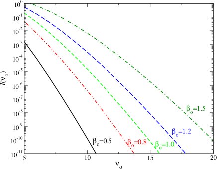
Figure 8: Values of ${\mathcal{I}}({\cal V}_{0})$ for $5\leq{\cal V}_{0}\leq 20$ and ${\cal S}=22$.

Taking the largest value of $\beta_{0}=0.56$ obtained for C₄H/C₄H^- with $\cal S$=10, $\langle\omega\rangle=0.01$ H, ${\cal V}_{0}=15$ and $\Lambda_{0}=0.13$, which is similar to the one obtained for CN/CN^- (see Fig. 7), we obtain

$$\langle\sigma_{c}\rangle\approx\frac{5\times 10^{-17}}{E_{el}}a_{0}^{2}\,,$$ (36)

where the energy is in hartree (H). At electron energy of 1 meV, the above formula gives the cross section of $10^{-12}\ a_{0}^{2}$. For somewhat more favorable situation, when $\cal S$=22 (as for C₈H) and a significantly larger $\beta_{0}=1$ (an arbitrary value, not necessarily representing C₈H/C₈H^-), the cross section at the same energy becomes larger, about $10^{-5}\ a_{0}^{2}$, but still remains small to explain the astrophysical observations.

V.2 Statistical distribution in the model

We consider here the distribution of different anion vibrational states after the electron capture if ${\cal V}_{0}$ is fixed. The electron capture probability into a vibrational state of the negative ion is proportional to the non-adiabatic coupling elements in Eq. (V.1). In this expression, $\beta_{s}^{2}\ll v_{s}$ in the factor $(\beta_{s}^{2}-v_{s})$ and, therefore, $\beta_{s}^{2}$ can be neglected. Making the change of variable $v_{s}\to v_{s}+1$ for the active mode in Eq. (V.1) and summing over all the modes, we obtain

$$|\bar{\Lambda}_{fi}|^{2}\approx({\cal V}_{0}+{\cal S}-1)\frac{\beta_{1}^{2v_{1}}\cdots\beta_{s}^{2v_{s}}\cdots\beta_{{\cal S}}^{2v_{{\cal S}}}}{v_{1}!\cdots v_{s}!\cdots v_{{\cal S}}!},$$ (37)

with the new condition that $v_{1}+\cdots+v_{\cal S}={\cal V}_{0}-1$. The most probable configuration {$v^{0}_{1},\cdots v^{0}_{\cal S}$} to capture an electron corresponds to an extremum of the function

$${\cal G}(v_{1}\cdots v_{{\cal S}})=\ln{|\bar{\Lambda}_{fi}|^{2}}-\lambda(\sum_{s=1}^{{\cal S}}v_{s}-{\cal V}_{0}+1),$$ (38)

where we use the method of Lagrange multipliers. Using the Stirling approximation,

$$\ln(v_{s}!)\approx v_{s}\ln\left(\frac{v_{s}}{e}\right)+\frac{1}{2}\ln(v_{s})+\ln(\sqrt{2\pi})\,,$$ (39)

the Lagrange equations, giving the extremum, become

$$\ln\beta_{s}^{2}-\ln v^{0}_{s}+\frac{1}{2v^{0}_{s}}-\lambda=0.$$ (40)

Typically, $\beta^{2}_{s}\ll 1$ and $v^{0}_{s}\geq 2$, thus the third term in (40) is much smaller than the first two terms and can, therefore, be discarded. Solving for $v^{0}$ we obtain

$$v^{0}_{s}\approx\left[\frac{\beta_{s}^{2}}{\beta_{0}^{2}}({\cal V}_{0}-1)\right],$$ (41)

where the brackets denote the closest integer number because $v^{0}_{s}$ should be an integer number. The modes with the largest separation between the equilibrium positions are, therefore, the most strongly excited in the electron capture, whereas bending modes barely contribute. However, if we consider the ${\cal S}_{str}=N-1$ stretching modes of a $N$-atoms carbon chain have similar displacements $\beta_{s}$, then the stretching modes will be equally populated with $\left[({\mathcal{V}}_{0}-1)/{\cal S}_{str}\right]$ quanta. Since we are interested in large carbon chains ${\cal S}_{str}\geq 4$, the optimum occupation numbers are such that $v_{s}^{0}\leq 4$. This result shows why the harmonic oscillator model is accurate for a carbon-chain molecule with several degrees of freedom. States with smallest possible number of excited quanta along each mode but involving many modes, contribute the most into the capture probability. Finally, only vibrational states with energies within the energy interval $[\langle E\rangle-\Delta E;\langle E\rangle+\Delta E]$ with $\Delta E=\hbar\Delta\omega\sqrt{{\cal V}_{0}-1}$ around energy $\langle E\rangle$ contribute significantly in the electron capture probability (see Appendix B). Because $\Delta\omega\approx 1000$ cm^-1, the energy spread is of the same order as the characteristic energy spacing $\Delta E_{c}$, such that the cross section of Eq. (35) should give a correct estimate of the electron capture cross section. Nonetheless, because the affinity of a negative ion can usually not be assigned exactly to one ${\cal V}_{0}$ value, Eq. (35) only gives an order of magnitude of the cross section.

V.3 Competition between radiative stabilization and autodetachment

For large molecules, once the electron is captured, in addition to the processes of autodetachment and spontaneous emission from the formed resonance, the system can also change its vibrational state. Although the energy of the system cannot change without emitting a photon, such a change in the vibrational excitation is possible because all vibrational levels in this energy region are in fact resonances and have finite widths. In large polyatomic molecules the coupling between vibrational modes could be strong, so one would expect that, at least, for some molecules a rapid change of the vibrational state is possible. If it happens that the autodetachment width of this new state is small or the probability of the spontaneous emission for this state is enhanced, for example, due to a better Franck-Condon overlap, one can expect that the system will not be able to loose rapidly the attached electron and will eventually be stabilized by emitting a photon. If this happens, then the IREA cross section (16) should be modified as

$$\sigma_{IREA}=\frac{\Gamma_{sp}+\Gamma_{vc}}{\Gamma_{tot}}\sigma_{c}\,,$$ (42)

where $\Gamma_{tot}$ now includes also the width $\Gamma_{vc}$ for the mentioned change of the vibrational state $\Gamma_{tot}=\Gamma_{sp}+\Gamma_{ad}+\Gamma_{vc}$. The time scale for change of vibrational state in a favorable case when the initial and final vibrational states strongly interact with each other, must be of the order of a vibrational period, in a ps range, which makes $\Gamma_{vc}$ dominant over the two other widths. In this limiting case, the IREA cross section $\sigma_{IREA}$ would be determined by its upper bound $\sigma_{c}$ of Eq. (15). Based on the above discussion, we can conclude that in the process of formation of negative ions C_mN^- ($m=1,3,5$) and C_nH^- ($n=2,4$) by radiative attachment, a significant contribution into the total REA cross section of the IREA is unlikely.

Non-adiabatic couplings in polyatomic molecules could be significant near a conical intersection of potential energy surfaces and, as a result, lead to a larger probability of electron capture during the first step of IREA. For the considered case of radiative attachment, this can happen for certain incident electron energies if (a) the neutral molecule has degenerate vibrational modes and (b) the formed electronic state of the anion is also degenerate. The linear carbon chain molecules C_nH ($n=2,4,6,8$) and C_mH ($m=3,5$) do have degenerate vibrational modes, and some of the corresponding anions may have excited electronic states of the degenerate ${}^{1}\Pi$ symmetry. If such excited electronic states have appropriate energies, an electron with $\pi$ symmetry, incident at the neutral target, could be captured due non-adiabatic Renner-Teller coupling, into the degenerate ${}^{1}\Pi$ state of the anion, exciting at the same time, the degenerate vibrational mode of the molecule. Such a process is similar to electron capture in dissociative recombination of linear molecules, HCO⁺ and N₂H⁺ Mikhailov et al. (2006); Douguet et al. (2008, 2009); Fonseca dos Santos et al. (2014), but there is an important difference: In collisions between an electron and a positive molecular ion, the density of electronic resonances is larger by several orders of magnitude. In dissociative recombination, electronic Rydberg resonances with a vibrationally excited core could be found virtually at any energy above the lowest ionization limit. But only a few molecular anions, such as C${}_{2}^{-}$, are known to have electronic resonances. Therefore, for a significant increase of the IREA cross section, the anion should have an electronic ${}^{1}\Pi$ state close to the energy of the initial continuum state of the $e^{-}-M$ system. This could, probably, be the case for one of the carbon chain anions, but it seems unlikely that all observed anions have an electronic resonance near the energy of the initial state of the $e^{-}-M$ system with small energy of the incident electron.

VI Conclusion

We have extended the theoretical approach to study the process of radiative electron attachment, developed in our previous study Fonseca dos Santos et al. (2014), to larger molecules. Using the approach we have calculated REA cross sections for the three negative molecular ions CN^-, C₂H^-, and C₄H^-. The following concluding remarks should be stressed as a result of the present study.

• For completeness of the approach, two pathways for the process have been considered: (1) In the direct pathway, the electron, incident on the molecule, emits a photon and forms a negative ion in one of the lowest vibrational levels. (2) The indirect pathway is a two-step process, for which the incident electron is initially captured through non-Born-Oppenheimer coupling into a vibrationally excited state of the anion, forming a resonance. As a second step in IREA, the resonant vibronic state of the anion emits a photon, which stabilizes the anion with respect to autodetachment. The contribution of the indirect pathway was found to be negligible compared to the direct mechanism if no unusual threshold effects, virtual states or vibrational Feshbach dipole resonances are present.

• The obtained REA rate coefficients evaluated at temperature 30 K are $7\times 10^{-16}$cm³/s for CN^-, $7\times 10^{-17}$cm³/s for C₂H^-, $2\times 10^{-16}$cm³/s for C₄H^-. The coefficients depend weakly on temperature between 10 K and 100 K and increase relatively fast with temperature above 200 K. The validity of the obtained results is verified by comparing the present theoretical results with experimental data from recent photodetachment experiments.

• Previously, it was believed that carbon-chain anions, C_nH^- ($n=2,4,6,8$) or C_mN^- ($m=3,5$), observed in the interstellar medium, are formed by the REA process. The REA rate coefficients obtained in this study are too small to explain the observed abundance of the anions in the ISM. For example, for C₄H^-, the magnitude of the rate coefficient needed to explain the observed abundance should be of the order of $10^{-10}$ cm³/s Herbst and Osamura (2008). Thus, the present results suggest that in the ISM, either dipole resonant states or non-local threshold effects increase drastically the REA cross section (and the rate of anion formation) or these anions are formed through a process different than REA.

Acknowledgments. This work is supported by the National Science Foundation, Grant No’s PHY-11-60611 and PHY-10-68785. Part of the material presented on this manuscript is based on work conducted while A. Orel was serving at NSF.

Appendix A Formula for density of states

A.1 Total number of states

We assume that we have $\cal S$ vibrational modes of the negative ion $M^{-}$, and the energy of quanta in different modes is approximately the same $\Delta E$. To reach energy $E_{i}+E_{el}$ of the initial state of the $M+e^{-}$ system, an excitation of $\cal V$ quanta is needed

$$\sum\limits_{s=1}^{\cal S}v_{s}={\cal V}\ \mathrm{with}\ v_{s}\geq 0\,.$$ (43)

The density of vibrational states of the $M^{-}$ anion near energy $E_{i}+E_{el}$ is evaluated as $N_{T}/\Delta E$, where $N_{T}$ is the number of combinations $\{v_{1},v_{2},\cdots,v_{\cal S}\}$ how the sum above can be formed.

To obtain the number of combinations $N_{T}$, it is convenient to represent $\cal V$ quanta as objects arranged in a row. The row of quanta is separated in subsets $v_{1},v_{2},\cdots,v_{\cal S}$ by ${\cal S}-1$ walls. Now we would like to count the number of possibilities how the ${\cal S}-1$ walls can be placed. We can place the first wall in ${\cal V}+1$ places between the objects, keeping in mind that we can also place it before the first or after the last quantum. The second wall can be placed at ${\cal V}+2$ different locations, because now we have ${\cal V}$ quanta plus the first wall in the row. (We will account later for the fact that the walls are identical). Continuing in this way, we obtain the total number $\prod\limits_{i=1}^{S-1}({\cal V}+i)=({\cal V+S}-1)!/{\cal V}!$ of possibilities of how the ${\cal S}-1$ distinguishable walls can be placed. Since the walls are all the same, we have to divide the product by the number $({\cal S}-1)!$ of permutations of the $({\cal S}-1)$ walls for a given partition of the row of ${\cal V}$. Thus, the number of combinations corresponding to the sum of Eq. (43) is

$$N_{T}={{{\cal V+S}-1}\choose{{\cal S}-1}}={{{\cal V+S}-1}\choose{{\cal V}}}\,.$$ (44)

A.2 Number of density of states when only $n$ modes are excited

We derive now the formula for the number of combinations corresponding to $n$ excited modes, given that there are $\cal S$ modes. For example, if only the first $n$ modes are excited, we have

$$\sum\limits_{s=1}^{n}v_{s}={\cal V}\ \mathrm{with}\ v_{s}>0\,.$$ (45)

In this situation, the number of combinations how the sum above can be formed is given by ${{{\cal V}-1}\choose{n-1}}$. To prove this it is again convenient to represent the $\cal V$ quanta as objects arranged in a row. The row of quanta is separated in groups of $v_{1}$, $v_{2},\cdots$, $v_{n}$ objects, by $n-1$ walls. Now we would like to count the number of possibilities such that $n-1$ walls can be placed. We can place the first wall in ${\cal V}-1$ places between the objects, keeping in mind that at the left and the right of the wall there were at least one quantum because $v_{s}>0$. The second wall cannot be placed at same the position, because it would mean that one of the $n$ modes will be inactive, i.e. $v_{s}=0$. Therefore, for the second wall there are ${\cal V}-2$ ways to place it. The total number of possibilities to place $n-1$ walls is, therefore, $\prod\limits_{i=1}^{n-1}({\cal V}-i)$. Since the walls are all the same, we have to divide the product by the number $(n-1)!$ of permutations of the identical $(n-1)$ walls for a given partition of the row of ${\cal V}$ objects. Thus, the number of combinations corresponding to the sum of Eq. (43) is indeed ${{{\cal V}-1}\choose{n-1}}$.

To obtain the total number of combinations $N_{n}$ when any $n$ modes are excited, we have to multiply the above number with the number of ways how $n$ modes can be chosen from the set of $\cal S$ modes. There are ${{{\cal S}}\choose{n}}$ such ways. Therefore,

$$N_{n}={{{\cal V}-1}\choose{n-1}}{{{\cal S}}\choose{n}}\,.$$ (46)

Finally, we will prove that the sum of $N_{n}$ gives the total number $N_{T}$ of vibrational states of Eq. (44), i.e. we will show that

$$N_{T}=\sum\limits_{n=1}^{\cal S}N_{n}\,.$$ (47)

It can be verified using Vandermonde’s identity, which states that

$${{m+l}\choose{r}}=\sum\limits_{n=0}^{r}{{m}\choose{n}}{{l}\choose{r-n}}\,.$$ (48)

In our case, we have

$$\sum\limits_{n=1}^{\cal S}N_{n} = \sum\limits_{n=1}^{\cal S}{{{\cal V}-1}\choose{n-1}}{{{\cal S}}\choose{n}}=\sum\limits_{n=0}^{\cal S^{\prime}}{{{\cal V}-1}\choose{n}}{{{{\cal S^{\prime}}+1}}\choose{n+1}}$$ (49)

$$= \sum\limits_{n=0}^{\cal S^{\prime}}{{{\cal V}-1}\choose{n}}{{{{\cal S^{\prime}}+1}}\choose{{\cal S^{\prime}}-n}}\,,$$

where ${\cal S^{\prime}}={\cal S}-1$. Now using Vandermonde’s identity with $m={\cal V}-1$, $l={\cal S^{\prime}}+1$ and $r=\cal S^{\prime}$, the sum is written

$$\sum\limits_{n=1}^{\cal S}N_{n}={{{\cal V+S}-1}\choose{{\cal S}-1}}\,,$$ (50)

which is indeed $N_{T}$ of Eq. (44).

Appendix B Closed-form expression for ${\mathcal{I}}({\cal V}_{0})$ and statistical formula

We will reduce ${\mathcal{I}}({\cal V}_{0})$ in Eq. (31) to a closed-form expression. In order to simplify the equations, we introduce the shorthand notation ${\bar{\mathcal{I}}}_{0}=2{\mathcal{I}}({\cal V}_{0})\exp({\beta_{0}^{2}})$. From Eq. (V.1), we decompose ${\bar{\mathcal{I}}}_{0}$ in three terms:

$${\bar{\mathcal{I}}}_{0} = \sum_{s=1}^{\cal S}\sum_{{\cal V}_{f}={\cal V}_{0}}\frac{\beta_{1}^{2v_{1}}\cdots\beta_{s}^{2v_{s}}\cdots\beta_{{\cal S}}^{2v_{{\cal S}}}}{v_{1}!\cdots v_{s}!\cdots v_{{\cal S}}!}$$ (51)

$$\times(\underbrace{\beta_{s}^{2}}_{1}-\underbrace{2v_{s}}_{2}+\underbrace{v_{s}^{2}/\beta_{s}^{2}}_{3})\,.$$

The under braces indicate the factors involved in each term, such that ${\bar{\mathcal{I}}}_{0}={\bar{\mathcal{I}}}_{1}+{\bar{\mathcal{I}}}_{2}+{\bar{\mathcal{I}}}_{3}$. For convenience, we introduce the function

$${\bar{\mathcal{Z}}(\beta_{1}\cdots\beta_{{\cal S}})}\equiv\sum_{{\cal V}_{f}={\cal V}_{0}}\frac{\beta_{1}^{2v_{1}}\cdots\beta_{s}^{2v_{s}}\cdots\beta_{{\cal S}}^{2v_{{\cal S}}}}{v_{1}!\cdots v_{s}!\cdots v_{{\cal S}}!}\,.$$ (52)

Recalling the multinomial theorem, this function takes the compact form

$${\bar{\mathcal{Z}}(\beta_{1}\cdots\beta_{{\cal S}})}=\frac{(\beta_{1}^{2}+\cdots+\beta^{2}_{\cal S})^{{\cal V}_{0}}}{{\cal V}_{0}!}=\frac{\beta_{0}^{2{\cal V}_{0}}}{{\cal V}_{0}!}\,.$$ (53)

The first term ${\bar{\mathcal{I}}}_{1}$ is expressed as

$${\bar{\mathcal{I}}}_{1}=\sum_{s=1}^{\cal S}\beta_{s}^{2}{\bar{\mathcal{Z}}(\beta_{1}\cdots\beta_{{\cal S}})}\,,$$ (54)

such that we readily obtain

$${\bar{\mathcal{I}}}_{1}=\frac{\beta_{0}^{2{\cal V}_{0}+2}}{{\cal V}_{0}!}\,.$$ (55)

The second term ${\bar{\mathcal{I}}}_{2}$ is written as

$${\bar{\mathcal{I}}}_{2}=-\sum_{s=1}^{\cal S}\sum_{{\cal V}_{f}={\cal V}_{0}}2v_{s}\frac{\beta_{1}^{2v_{1}}\cdots\beta_{s}^{2v_{s}}\cdots\beta_{{\cal S}}^{2v_{{\cal S}}}}{v_{1}!\cdots v_{s}!\cdots v_{{\cal S}}!}\,,$$ (56)

which takes the convenient form

$${\bar{\mathcal{I}}}_{2}=-\sum_{s=1}^{\cal S}\frac{\partial\bar{\mathcal{Z}}(\beta_{1}\cdots\beta_{{\cal S}})}{\partial\ln\beta_{s}}\,.$$ (57)

Using the value of ${\bar{\mathcal{Z}}(\beta_{1}\cdots\beta_{{\cal S}})}$ in Eq. (53), we obtain the following expression:

$${\bar{\mathcal{I}}}_{2}=-\frac{2{\cal V}_{0}\beta_{0}^{2{\cal V}_{0}}}{{\cal V}_{0}!}\,.$$ (58)

The last term ${\bar{\mathcal{I}}}_{3}$ is clearly the dominant one, with the slightly more complicated form:

$${\bar{\mathcal{I}}}_{3}=\sum_{s=1}^{\cal S}\sum_{{\cal V}_{f}={\cal V}_{0}}\frac{v^{2}_{s}}{\beta^{2}_{s}}\frac{\beta_{1}^{2v_{1}}\cdots\beta_{s}^{2v_{s}}\cdots\beta_{{\cal S}}^{2v_{{\cal S}}}}{v_{1}!\cdots v_{s}!\cdots v_{{\cal S}}!}\,.$$ (59)

Note that the apparent indeterminacy is easily removed for a degenerate mode by taking the limit $\beta_{s}\to 0$ in Eq. (59). Applying a similar method, we find

$${\bar{\mathcal{I}}}_{3}=\frac{1}{4}\sum_{s=1}^{\cal S}\frac{1}{\beta^{2}_{s}}\frac{\partial^{2}{\bar{\mathcal{Z}}(\beta_{1}\cdots\beta_{{\cal S}})}}{\partial(\ln\beta_{s})^{2}}\,,$$ (60)

and thus we conclude that

$${\bar{\mathcal{I}}}_{3}=\frac{{\cal V}_{0}({\cal V}_{0}+{\cal S}-1)\beta_{0}^{2{\cal V}_{0}-2}}{{\cal V}_{0}!}\,.$$ (61)

Finally, the closed-form formula for ${\mathcal{I}}({\cal V}_{0})$ is given by:

$${\mathcal{I}}({\cal V}_{0})=\frac{\beta_{0}^{2{\cal V}_{0}-2}\left[({\cal V}_{0}-\beta_{0}^{2})^{2}+{\cal V}_{0}({\cal S}-1)\right]}{{\cal V}_{0}!}\frac{e^{-\beta_{0}^{2}}}{2}.$$ (62)

In the above expression, $\beta^{2}_{0}\ll{\cal V}_{0}$, which allows us to simplify the expression as

$${\mathcal{I}}({\cal V}_{0})\approx\frac{({\cal V}_{0}+{\cal S}-1)}{({\cal V}_{0}-1)!}\frac{\beta_{0}^{2{\cal V}_{0}-2}e^{-\beta_{0}^{2}}}{2}\,.$$ (63)

We also derive an expression for the average total energy of the system, weighted over the electron capture transition probabilities, given that ${\cal V}_{0}$ quanta are excited. First, neglecting the terms $\beta_{s}^{2}\ll v_{s}$ in Eq. (V.1), the transition probabilities to capture in an anion vibrational state are proportional to

$${\cal P}(\beta_{1}\cdots\beta_{\cal S})=v_{s}\frac{\beta_{1}^{2v_{1}}\cdots\beta_{s}^{2v_{s}-2}\cdots\beta_{{\cal S}}^{2v_{{\cal S}}}}{v_{1}!\cdots(v_{s}-1)!\cdots v_{{\cal S}}!}.$$ (64)

Therefore, the partition function used to normalize the probabilities takes the form

$$\Xi=\sum_{s=1}^{\cal S}\sum_{{\cal V}_{f}={\cal V}_{0}}{\cal P}(\beta_{1}\cdots\beta_{\cal S})=\bar{{\cal I}}_{3}\,.$$ (65)

and the average energy is thus expressed as

$$\langle E\rangle = \frac{1}{\Xi}\sum_{{\cal V}_{f}={\cal V}_{0}}E_{f}{\cal P}(\beta_{1}\cdots\beta_{\cal S})\,,$$ (66)

where $E_{f}=\hbar(v_{1}\omega_{1}+\cdots+v_{{\cal S}}\omega_{{\cal S}})$ is the energy of the vibrational state $|\chi_{f}\rangle$ (the anion ground state is chosen as the reference energy). After some straightforward manipulations, we obtain for ${\cal V}_{0}>1$ the expression

$$\langle E\rangle \approx ({\cal V}_{0}-1)\hbar\langle\omega\rangle,$$ (67)

where $\langle\omega\rangle=\frac{1}{\beta_{0}^{2}}\sum\beta_{s}^{2}\omega_{s}$ is an average vibrational frequency weighted over the displacements $\beta_{s}$. In a similar fashion, one can calculate the energy spread $\Delta E=\sqrt{\langle E^{2}\rangle-\langle E\rangle^{2}}$ around the average energy $\langle E\rangle$, which takes the value

$$\Delta E\approx\hbar\Delta\omega\sqrt{{\cal V}_{0}-1},$$ (68)

where $\Delta\omega=\sqrt{\langle\omega^{2}\rangle-\langle\omega\rangle^{2}}$ is the vibrational frequency spread, with $\langle\omega^{2}\rangle=\frac{1}{\beta_{0}^{2}}\sum\beta_{s}^{2}\omega^{2}_{s}$.

References

- McCarthy et al. (2006) M. C. McCarthy, C. A. Gottlieb, H. Gupta, and P. Thaddeus, Ap. J. Lett. 652, L141 (2006).
- Cernicharo et al. (2007) J. Cernicharo, M. Guelin, M. Agundez, K. Kawaguchi, and P. Thaddeus, A&A 61, L37 (2007).
- Herbst and Osamura (2008) E. Herbst and Y. Osamura, Ap. J. 679, 1670 (2008).
- Harada and Herbst (2008) N. Harada and E. Herbst, Ap. J. 685, 272 (2008).
- Cernicharo et al. (2008) J. Cernicharo, M. Guélin, M. Agúndez, M. C. McCarthy, and P. Thaddeus, Astrophys. J. Lett. 688, L83 (2008).
- H. Gupta and S. Brünken and F. Tamassia and C. A. Gottlieb and M. C. McCarthy and P. Thaddeus (2007) H. Gupta and S. Brünken and F. Tamassia and C. A. Gottlieb and M. C. McCarthy and P. Thaddeus, Astrophys. J. Lett. 655, L57 (2007).
- Kawaguchi et al. (2007) K. Kawaguchi, R. Fujimori, S. Aimi, S. Takano, E. Y. Okabayashi, H. Gupta, S. Bruenken, C. A. Gottlieb, M. C. Mccarthy, and P. Thaddeus, Publ. Astron. Soc. Japan 59, L47 (2007).
- Thaddeus et al. (2008) P. Thaddeus, C. A. Gottlieb, H. Gupta, S. Brunken, M. C. McCarthy, M. Agundez, M. Guelin, and J. Cernicharo, Ap. J. 677, 1132 (2008).
- Agúndez et al. (2010) M. Agúndez, J. Cernicharo, M. Guélin, C. Kahane, E. Roueff, J. Klos, F. Aoiz, F. Lique, N. Marcelino, J. Goicoechea, et al., A&A 517, L2 (2010).
- McDowell (1961) M. McDowell, Observatory 81, 240 (1961).
- Dalgarno and McCray (1973) A. Dalgarno and R. McCray, Astrophys. J. 181, 95 (1973).
- Herbst (1981) E. Herbst, Nature 289, 656 (1981).
- Herbst (1985) E. Herbst, A&A 153, 151 (1985).
- R. Terzieva and E. Herbst (2000) R. Terzieva and E. Herbst, Int. J. Mass. Spectrom. 201, 135 (2000).
- Petrie and Herbst (1997) S. Petrie and E. Herbst, Astrophys. J. 491, 210 (1997).
- Millar et al. (2007) T. J. Millar, C. Walsh, M. A. Cordiner, R. N. Chuimín, and E. Herbst, Ap. J. 662, L87 (2007).
- Petrie (1996) S. Petrie, Mon. Not. R. Astron. Soc. 281, 137 (1996).
- Douguet et al. (2013) N. Douguet, S. Fonseca dos Santos, M. Raoult, O. Dulieu, A. Orel, and V. Kokoouline, Phys. Rev. A 88, 052710 (2013).
- Kumar et al. (2013) S. Kumar, D. Hauser, R. Jindra, T. Best, Š. Roučka, W. Geppert, T. Millar, and R. Wester, Astrophys. J. 776, 25 (2013).
- Best et al. (2011) T. Best, R. Otto, S. Trippel, P. Hlavenka, A. von Zastrow, S. Eisenbach, S. Jezouin, R. Wester, E. Vigren, M. Hamberg, et al., Astrophys. J. 742, 63 (2011).
- C. W. McCurdy and T. N. Rescigno (1989) C. W. McCurdy and T. N. Rescigno, 39, 4487 (1989).
- Orel et al. (1991) A. E. Orel, T. Rescigno, and B. Lengsfield, Phys. Rev. A 44, 4328 (1991).
- Douguet et al. (2014) N. Douguet, V. Kokoouline, and A. E. Orel, Phys. Rev. A 90, 063410 (2014).
- Wigner (1948) E. P. Wigner, Phys. Rev. 73, 1002 (1948).
- Friedrich (2006) H. Friedrich, Theoretical atomic physics (Springer, 2006).
- Bradforth et al. (1993) S. E. Bradforth, E. H. Kim, D. W. Arnold, and D. M. Neumark, J. Chem. Phys. 98, 800 (1993).
- Ervin and Lineberger (1991) K. Ervin and W. Lineberger, J. Chem. Phys. 95, 1167 (1991).
- Zhou et al. (2007) J. Zhou, E. Garand, and D. M. Neumark, J. Chem. Phys. 127, 114313 (2007).
- Taylor et al. (1998) T. R. Taylor, C. Xu, and D. M. Neumark, J. Chem. Phys. 108 (1998).
- Güthe et al. (2001) F. Güthe, M. Tulej, M. V. Pachkov, and J. P. Maier, Astrophys. J. 555, 466 (2001).
- Carelli et al. (2014) F. Carelli, F. A. Gianturco, R. Wester, and M. Satta, J. Chem. Phys. 141, 054302 (2014).
- Frank et al. (1999) A. Frank, R. Lemus, and F. Pérez-Bernal, J. Math. Chem. 25, 383 (1999).
- Mikhailov et al. (2006) I. A. Mikhailov, V. Kokoouline, A. Larson, S. Tonzani, and C. H. Greene, Phys. Rev. A 74, 032707 (2006).
- Douguet et al. (2008) N. Douguet, V. Kokoouline, and C. H. Greene, Phys. Rev. A 77, 064703 (2008).
- Douguet et al. (2009) N. Douguet, V. Kokoouline, and C. H. Greene, Phys. Rev. A 80, 062712 (2009).
- Fonseca dos Santos et al. (2014) S. Fonseca dos Santos, N. Douguet, V. Kokoouline, and A. Orel, J. Chem. Phys. 140, 164308 (2014).