Control of transversal instabilities in reaction-diffusion systems

Abstract

In two-dimensional reaction-diffusion systems, local curvature perturbations in the shape of traveling waves are typically damped out and disappear in the course of time. If, however, the inhibitor diffuses much faster than the activator, transversal instabilities can arise, leading from flat to folded, spatio-temporally modulated wave shapes and to spreading spiral turbulence. For experimentally relevant parameter values, the photosensitive Belousov-Zhabotinsky reaction (PBZR) does not exhibit transversal wave instabilities. Here, we propose a mechanism to artificially induce these instabilities via a wave shape dependent spatio-temporal feedback loop, and study the emerging wave patterns. In numerical simulations with the modified Oregonator model for the PBZR using experimentally realistic parameter values we demonstrate the feasibility of this control scheme. Conversely, in a piecewise-linear version of the FitzHugh-Nagumo model transversal instabilities and spiral turbulence in the uncontrolled system are shown to be suppressed in the presence of control, thereby stabilising flat wave propagation.

Keywords: traveling waves, control, transversal instabilities

1 Introduction

A large variety of pattern forming processes can be understood in terms of the advancement of an interface between two or more spatial domains. An interface that becomes unstable to diffusion possibly causes intricate spatio-temporal dynamics. Well known examples include the Mullins-Sekerka instability during crystal growth and formation of snow flakes [1, 2], and the Saffman-Taylor instability leading to viscous fingering in multiphase flow and porous media [3, 4, 5]. Other phenomena affected by interfacial instabilities are flame fronts [6, 7], Marangoni convection [8], and growing cell monolayers [9].
Traveling plane waves in excitable media exhibit interfacial instabilities as well. Here, an effective interface separates the excited state from the excitable rest state. A straight isoconcentration line of a two-dimensional flat wave can suffer an instability leading to stationary or time dependent modulations orthogonal to the propagation direction. Further away from the instability threshold, rotating wave segments and spreading spiral turbulence are observed [10, 11]. For standard activator-inhibitor kinetics, these so-called transversal or lateral wave instabilities typically occur if the inhibitor diffuses much faster than the activator. This result was analytically predicted first by Kuramoto for piecewise-linear reaction kinetics [12, 13]. Later, it was confirmed numerically by Horváth et al. for autocatalytic reaction-diffusion fronts with cubic reaction kinetics [14] as well as in experiments with the iodate-arsenous acid reaction [15] and the acid-catalyzed chlorite–tetrathionate reaction [16].
The experimental workhorse of chemical pattern formation, the Belousov-Zhabotinsky (BZ) reaction, does typically not display transversal wave instabilities. Dispersing the reagents of the BZ reaction in nanodroplets of a water-in-oil microemulsion allows to increase the inhibitor diffusivity considerably [17] and leads, for example, to segmented spiral waves as reported by Vanag and Epstein [18]. Even in the presence of an electrical field applied to enhance transversal instabilities in cubic autocatalytic reaction-diffusion fronts, the inhibitor diffusion coefficient is always required to be sufficiently larger than that of the activator [19, 20, 21].
Because of the possibility to apply spatio-temporal external forcing or feedback-mediated control loops by exploiting the dependence of the local excitation threshold on the intensity of applied illumination, the photosensitive variant of the BZ reaction has been widely used as a paradigm of an experimentally well controllable RD system. So far, unstable wave propagation has been stabilised by global feedback [22]. Two feedback loops were used to stabilise unstable wave segments and to guide their propagation along pre-given trajectories [23]. Also, spiral wave drift in response to resonant external forcing and various feedback-mediated control loops has been extensively studied experimentally in PBZR systems, compare for example [24, 25, 26, 27, 28].
In this paper, we design a curvature-dependent spatio-temporal feedback loop in order to destabilise a stable propagating planar reaction-diffusion wave by inducing transversal instabilities. In numerical simulations with the modified Oregonator model for the PBZR, we study the wave patterns emerging beyond the instability threshold, and demonstrate the capability to actively select wave patterns by modifying feedback parameters accessible to the experimenter. Conversely, under conditions where planar wave propagation fails due to transversal instabilities, using the same feedback mechanism we suppress ongoing breakup and segmentation of waves, thereby stabilising unstable propagating planar waves.

2 Theory

2.1 Models

The first model we investigate is the three component modified Oregonator model [29]

$$\frac{\partial u}{\partial t} = \frac{1}{\epsilon}\left[u-u^{2}+w\left(q-u\right)\right]+D_{u}\Delta u,$$ (1)

$$\frac{\partial v}{\partial t} = u-v,$$ (2)

$$\frac{\partial w}{\partial t} = \frac{1}{\tilde{\epsilon}}\left[\Phi+fv-w\left(u+q\right)\right]+D_{w}\Delta w.$$ (3)

Here, the parameters $\epsilon$ and $\tilde{\epsilon}$ characterise the time scales for the dynamics of the activator $u$ and inhibitor $w$, respectively, and the stoichiometric parameters $q$ and $f$ depend on the temperature and chemical composition. All parameter values used in numerical simulations are listed in table 1 in A. The modified Oregonator model describes the light-sensitive Belousov-Zhabotinsky (BZ) reaction. In experiments, the catalyst $v$ can be immobilised in a gel and therefore the corresponding diffusion coefficient is set to zero. The activator $u$ and inhibitor $w$ diffuse with diffusion coefficients $D_{u}$ and $D_{w}$, whose ratio for typical BZ recipes is approximately $D_{w}/D_{u}\approx 1.2$. This value is too low to support transversal instabilities such that plane waves are stable for typical BZ recipes. The parameter $\Phi$ in equation (3) is proportional to the applied light intensity and measures the local excitation threshold. In experiments, spatio-temporal modulations of $\Phi$ can be applied to control wave propagation in the BZ reaction [23, 27, 28, 22].
Because the modified Oregonator model does not exhibit transversal instabilities in the parameter regime relevant for experiments, we investigate a second model. The piecewise-linear caricature of the FitzHugh-Nagumo (FHN) model [30, 11] received some attention in the context of transversal instabilities [11]. It is a two component model of standard activator-inhibitor type,

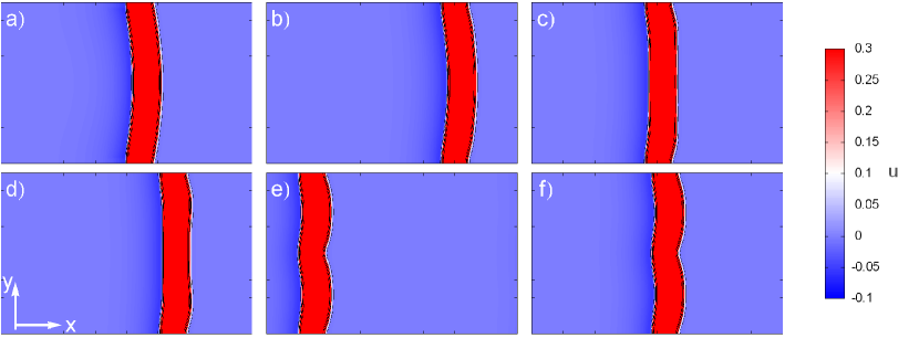
Figure 1: Slightly beyond the onset of transversal instabilities, an initially plane wave in the piecewise linear FitzHugh-Nagumo model develops a stationary fold. From left to right, top to bottom: time sequence of snapshots of a video which can be found in the Supplemental Material [31] for (a) $t=100$, (b) $t=320$, (c) $t=370$, (d) $t=420$, (e) $t=470$, and (f) $t=570$ for the parameters $\sigma=2.1,\,\epsilon=0.1425,\,a=0.1$. Computations were carried out with a constant time step $\Delta t=0.00001$ and space step $\Delta x=0.15$. The domain size is $160\times 90$.

$$\frac{\partial u}{\partial t} = \triangle u+F\left(u,v\right),$$ (4)

$$\frac{\partial v}{\partial t} = \sigma\triangle v+\epsilon G\left(u,v\right),$$ (5)

with $u$ being the activator and $v$ the inhibitor. The reaction kinetics are a piecewise-linear caricature of the FHN model

$$F\left(u,v\right) = f\left(u\right)-v,$$ (6)

$$G\left(u,v\right) = k_{g}u-v,$$ (7)

where

$$f\left(u\right)=\left\{\begin{array}[]{@{}l@{\quad}l}-k_{1}u,&u<\delta,\\ k_{f}\left(u-a\right),&\delta<u<1-\delta,\\ k_{2}\left(1-u\right),&1-\delta<u.\end{array}\right.$$ (8)

The parameters $k_{1}$ and $k_{2}$ are chosen such that $f\left(u\right)$ is continuous at $u=\delta$ and $u=1-\delta$, which leads to

$$k_{1} = \frac{k_{f}}{\delta}\left(a-\delta\right),\qquad k_{2}=\frac{k_{f}}{\delta}\left(1-\delta-a\right).$$ (9)

The remaining parameters for the function $f$ are chosen in such a way that $f$ resembles the cubic shape of the FHN activator nullcline. All parameter values used in numerical simulations are listed in table 2 in A. The parameter $a$ is a measure for the excitation threshold and used as the feedback parameter.
For numerical simulations, we assume an elongated two-dimensional channel of width $L$ in the $y$-direction with waves propagating in the $x$-direction. The boundary conditions in the $x$-direction are periodic while we assume periodic or Neumann boundary conditions in the $y$-direction. For both models, we use a box-like initial condition of width $b$ for the vector of components $\mathbf{u}$,

$$\mathbf{u}\left(x,y,t_{0}\right) = \Theta_{\text{Box}}\left(\left(x-\phi\left(y,t_{0}\right)\right)/b\right)\left(\mathbf{u}_{\text{max}}-\mathbf{u}_{0}\right)+\mathbf{u}_{0},$$ (10)

where $\mathbf{u}_{\text{max}}$ is the initial height of the pulse and $\mathbf{u}_{0}$ is the stationary point of the reaction kinetics. The box function is defined as

$$\Theta_{\text{Box}}\left(x\right)=\left\{\begin{array}[]{@{}l@{\quad}l}1,&\left|x\right|<1/2,\\ 0,&\left|x\right|\geq 1/2.\end{array}\right.$$ (11)

The initial shape of the wave is given by

$$\phi\left(y,t_{0}\right) = d-A\cos\left(\frac{2\pi y}{L}\right)\text{,}$$ (12)

where $A$ denotes the amplitude of deviation of the shape from a plane wave and $d$ is an offset. For numerical simulations in two spatial dimensions, we use Euler forward for the time evolution and a five point stencil for the Laplacian.
A phase diagram for the occurrence of transversal instabilities in the $\epsilon$-$\sigma$-parameter plane of the piecewise-linear FHN model was presented by Zykov et al. in [11]. Increasing the inhibitor diffusion coefficient $\sigma$ crosses the threshold for transversal instabilities. Shortly beyond the onset of transversal instabilities, a plane wave develops a fold which is stationary in a comoving frame of reference, see figure 1 for a time sequence of snapshots and the supplemental material [31] for a movie. Further away from the instability threshold, a plane wave breaks into segments which undergo self-sustained rotatory motion accompanied by permanent merging and annihilation of segments. This regime is also known as spreading spiral turbulence [11], see figure 2 for a time sequence of snapshots.

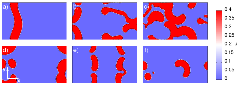
Figure 2: Segmentation of initially plane waves and spreading spiral turbulence occurs deep in the regime of transversal instabilities in the piecewise linear FitzHugh-Nagumo model. Parameter values as in figure 1 except $\epsilon=0.1575$. The segments undergo self-sustained rotatory motion and nucleate new waves. From left to right, top to bottom: snapshots of a video [31] for (a) $t=5$, (b) $t=301$, (c) $t=500$, (d) $t=672$, (e) $t=700$, and (f) $t=891$. The domain size is $160\times 90$.

2.2 Evolution equations for isoconcentration lines

Theoretically, the onset of transversal instabilities can be understood with the help of the linear eikonal equation

$$c_{n}\left(s,t\right) = c-\nu\kappa\left(s,t\right),$$ (13)

an evolution equation for a two-dimensional curve $\boldsymbol{\gamma}\left(s,t\right)=\left(\gamma_{x}\left(s,t\right),\gamma_{y}\left(s,t\right)\right)^{T}$ representing an isoconcentration line parametrised by the curve parameter $s$. The linear eikonal equation relates the normal velocity ($\boldsymbol{n}$ is the normal vector of $\boldsymbol{\gamma}$)

$$c_{n}\left(s,t\right) = \boldsymbol{n}\left(s,t\right)\cdot\partial_{t}\boldsymbol{\gamma}\left(s,t\right)$$ (14)

along $\boldsymbol{\gamma}$ linearly to its curvature,

$$\kappa\left(s,t\right) = \frac{\partial_{s}\gamma_{x}\left(s,t\right)\partial_{s}^{2}\gamma_{y}\left(s,t\right)-\partial_{s}\gamma_{y}\left(s,t\right)\partial_{s}^{2}\gamma_{x}\left(s,t\right)}{\left(\left(\partial_{s}\gamma_{x}\left(s,t\right)\right)^{2}+\left(\partial_{s}\gamma_{y}\left(s,t\right)\right)^{2}\right)^{3/2}}.$$ (15)

The curvature is conventionally assumed to be positive for convex isoconcentration lines, i.e., an isoconcentration lines with a protrusion in the propagation direction. The constant $c$ corresponds to the pulse velocity of a one-dimensional solitary wave and $\nu$ is the curvature coefficient. A rigorous derivation of the eikonal equation (13) from the reaction-diffusion system identifies the constant $\nu$ in terms of the one-dimensional pulse profile, its response function and the matrix of diffusion coefficients, see [32] for details. For a plane wave, any isoconcentration level is a straight line and therefore its curvature vanishes, $\kappa\left(s,t\right)\equiv 0$, everywhere along $\boldsymbol{\gamma}$. The stability of a plane wave is determined by the sign of the curvature coefficient $\nu$. As long as $\nu>0$, any point along the isoconcentration line of a convex bulge moves slower than a plane wave, while points of a concave dent move faster than a plane wave, thereby smoothing out deviations from a plane wave. If $\nu<0$, a convex bulge moves faster than a plane wave, protruding the bulge even further and thereby leading to an ever increasing curvature: a transversal instability arises. Patterns arising for $\nu<0$ cannot be described by the linear eikonal equation and terms depending nonlinearly on the curvature have to be taken into account which saturate the growth of an ever increasing curvature. At least two different nonlinear versions of equation (13) exist in the literature. Zykov et al. [33, 30, 34, 35] renormalised $\epsilon$ and $\sigma$ in equation (5) to derive a renormalised one-dimensional velocity $c$ depending on the curvature. Dierckx et al. [32] derive higher order nonlinear corrections in the curvature by a rigorous perturbation expansion with a small parameter proportional to the curvature, additionally generalising the eikonal equation to anisotropic media.
Apart from nonlinear eikonal equations, which are difficult to solve numerically, patterns arising beyond the threshold of transversal instability can be described by the Kuramoto-Sivashinsky (KS) equation,

$$\partial_{t}\phi\left(y,t\right) = c+\frac{c}{2}\left(\partial_{y}\phi\left(y,t\right)\right)^{2}+\nu\partial_{y}^{2}\phi\left(y,t\right)-\lambda\partial_{y}^{4}\phi\left(y,t\right).$$ (16)

Equation (16) is an evolution equation for the $x$-component $\phi\left(y,t\right)$ of an isoconcentration line $\boldsymbol{\gamma}$ parametrised in the form $\boldsymbol{\gamma}\left(y,t\right)=\left(\phi\left(y,t\right),y\right)^{T}$. See [13] and [36] for a derivation of equation (16) from a general RD system. The case of Neumann boundary conditions in the $y$-direction for the RD system imply that any isoconcentration line of activator and inhibitor meets the domain boundary in a right angle. This corresponds to Neumann boundary conditions for $\phi$,

$$\partial_{y}\phi\left(0,t\right) =0,\, \partial_{y}\phi\left(L,t\right)=0.$$ (17)

Similarly, periodic boundary conditions in the $y$-direction of the RD system carry over to periodic boundary conditions for $\phi$. Equation (16) was originally proposed by Sivashinsky [6] in the study of turbulent flame propagation and adapted for reaction-diffusion systems by Kuramoto [37, 13]. The parameter $\lambda$ can be expressed in terms of a sum over all eigenfunctions of the linear stability operator arising through a linearisation of the one-dimensional RD system around the traveling wave solution [13]. To compute $\lambda$, we use a method which avoids the virtually impossible numerical computation of all eigenfunctions, see [36] for details. The values of $\lambda$ and $\nu$ for the modified Oregonator model with parameters as given in A are

$$\lambda= 0.68,\qquad \nu=1.05.$$ (18)

The Kuramoto-Sivashinsky equation (16) allows a refined investigation of the onset of transversal instabilities. For a stability analysis of a plane wave in channel of width $L$ with Neumann boundary conditions, we apply a perturbation expansion in $0<\hat{\epsilon}\ll 1$ with an ansatz in form of a Fourier series,

$$\phi\left(y,t\right) = ct+\hat{\epsilon}\sum_{n=-\infty}^{\infty}a_{n}\exp\left(\omega_{n}t\right)\cos\left(\frac{\pi ny}{L}\right),$$ (19)

where the term $ct$ corresponds to a plane wave solution to the RD system traveling in the $x$-direction. The dispersion relation follows as

$$\omega_{n} = -\lambda\left(\frac{n\pi}{L}\right)^{4}-\nu\left(\frac{n\pi}{L}\right)^{2}.$$ (20)

Transversal instabilities occur only if $\omega_{1}>0$, i.e., $\nu$ must be negative and the channel width must exceed

$$L = \pi\sqrt{\frac{\lambda}{-\nu}}.$$ (21)

Thus, in general, the onset of a transversal instability depends on the boundary conditions and can be suppressed in thin channels. It is a long-wavelength instability, i.e., the first mode which becomes unstable upon reaching the threshold is the mode with the longest possible wavelength.
If $\nu<0$, the fourth order term in the KS equation (16) counteracts the negative diffusion term and leads to a saturation of the growth of wavefront modulations.Starting at the threshold of instability, the solution to the KS equation(16) displays a fold with a minimum located at $y=L/2$. Upon increasing $L$, this steady wave loses stability via a supercritical Hopf bifurcation [14] and the wave front starts to oscillate back and forth in a symmetrical fashion. Increasing $L$ even further leads to a symmetry breaking bifurcation with asymmetrical oscillations followed by a period doubling cascade to fully developed spatio-temporal chaos. In this regime, the KS equation displays a strong dependence on the initial data, with small differences in the initial conditions leading to dramatically different future time evolution. This characteristic of the KS equation is also studied as an analogy for hydrodynamic turbulence [38].
As long as $\nu>0$, no instability can arise and the fourth order term can be safely neglected by setting $\lambda=0$. In this case, equation (16) simplifies to the nonlinear phase diffusion equation, which in turn can be transformed to the usual diffusion equation via the Cole-Hopf transform [12]. Therefore, equation (16) with $\lambda=0$ can be solved analytically for arbitrary initial and boundary conditions.
To assess the accuracy of the Kuramoto-Sivashinsky equation (16) as an approximation for propagating reaction-diffusion waves, we compare the transition from an initially curved shape to a plane wave for $\nu>0$ with numerical simulations of the underlying two-dimensional modified Oregonator model Eqs. (1)-(3). The isoconcentration line $\boldsymbol{\gamma}$ of the activator variable $u$ is determined numerically as the set of points $\mathbf{r}=\left(x,\,y\right)^{T}$ for which $u\left(\mathbf{r},t\right)=u_{c}=0.2$. We compute the $x$-component of the wave’s centre of mass in a comoving frame as

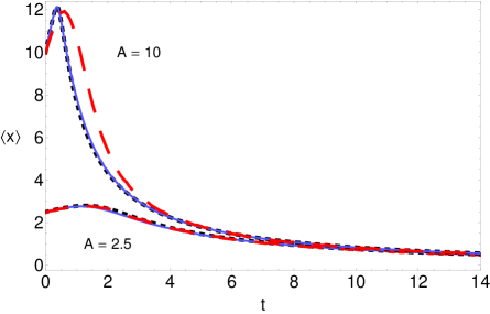
Figure 3: Time evolution of the mean $x$-coordinate of an isoconcentration line in a comoving frame of reference. Comparison of Kuramoto-Sivashinsky equation (black dotted line), nonlinear phase-diffusion equation (blue line) and for the activator isoconcentration line with $u\left(x,y,t\right)=0.2$ of the modified Oregonator obtained by numerical simulations (red dotted line).

$$\left\langle x\right\rangle\left(t\right) = \frac{1}{L}\intop_{0}^{L}\phi\left(y,t\right)dy-\phi\left(0,t\right).$$ (22)

Figure 3 shows the time evolution of $\left\langle x\right\rangle\left(t\right)$ obtained from the Kuramoto-Sivashinsky equation (black dotted line) and nonlinear phase diffusion equation (blue solid line) and for the modified Oregonator model obtained by numerical simulations (red dashed line) for two different values of the amplitude $A$ which characterises the initial deviation from a plane wave. As one would expect intuitively, the agreement between numerical simulations on the one hand and Kuramoto-Sivashinsky equation and nonlinear phase diffusion equation on the other hand becomes worse the larger is the initial amplitude $A$. For large times, i.e., when the curved isoconcentration line approaches a straight line, all results agree. The nonlinear phase diffusion equation and the Kuramoto-Sivashinsky equation practically yield the same result for all times, confirming the fact that the fourth order derivative in the Kuramoto-Sivashinsky equation can safely be neglected if the curvature coefficient is $\nu>0$.

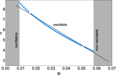
Figure 4: Velocity $c$ of a one-dimensional solitary pulse over the parameter $\Phi$ proportional to applied light intensity for the modified Oregonator model. The result of numerical simulations (blue dots) can be well approximated by a linear least square fit (blue solid line).

2.3 Curvature-dependent feedback control

The feedback law proposed in this article requires that the velocity $c$ of a one-dimensional wave depends sufficiently strongly on a parameter which can be controlled in experiments. For the modified Oregonator model, we use the parameter $\Phi$ proportional to the applied light intensity as the feedback parameter. A numerical computation of the dependence of $c$ on $\Phi$ is shown in figure 4. With relatively good accuracy, the dependence can be assumed to be linear,

$$c\left(\Phi\right) = c_{0}+c_{1}\Phi,$$ (23)

with parameters $c_{1}=-90.191,\,c_{0}=9.013$ obtained from a least square fit. Solitary waves exist only in the excitable regime of $\Phi$ values indicated by the dashed lines in figure 4. For $\Phi\lesssim 0.045$, the rest state is unstable and the medium becomes oscillatory. For $\Phi\gtrsim 0.068$, the solitary pulse profile becomes unstable and decays to the stable rest state. A successful feedback control is possible if $\Phi$ is restricted to lie between these two values.

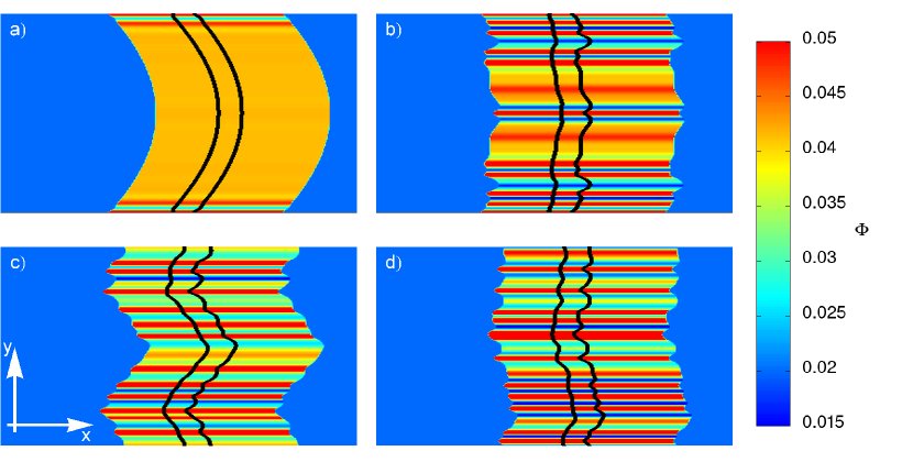
Figure 5: Small modulations of the wave shape occur for weak feedback with an effective curvature coefficient of $\tilde{\nu}=-0.75$. Snapshots of a movie [31] for (a) $t=3.5$, (b) $t=10.6$, (c) $t=25.2$, and (d) $t=69.3$. Colours denote the value of the applied spatio-temporal illumination field $\Phi\left(x,y,t\right)$ which is proportional to the curvature of the black isoconcentration line. Shown are clippings of size $21.5\times 30$ centred on the wave’s centre of mass while the computational domain is $110\times 30$. This and the following computations of the modified Oregonator model were carried out with a time step size of $\Delta t=0.0001$ and a space step size $\Delta x=0.05$. Parameter values for the feedback law are $\Phi_{\text{min}}=0.018,\,\Phi_{\text{max}}=0.042$.

We introduce a feedback law for $\Phi$ depending linearly on the curvature,

$$\Phi\left(\kappa\right) = \alpha+\beta\kappa.$$ (24)

The parameters $\alpha$ and $\beta$ are accessible to an experimenter. In general, these parameters can be adjusted with time to achieve a better performance of the control. Together with equation (23) and equation (24), the linear eikonal equation (13) becomes

$$c_{n} = c_{1}\alpha+c_{0}-\tilde{\nu}\kappa,$$ (25)

with the effective curvature coefficient

$$\tilde{\nu}=\nu-c_{1}\beta.$$ (26)

Depending on the sign of $\tilde{\nu}$, the control will have very different effects. If a plane wave is stable with respect to transversal perturbations because $\nu>0$, we can excite transversal instabilities if $\tilde{\nu}=\nu-c_{1}\beta<0$. Conversely, if $\nu>0$ such that plane waves are unstable with respect to transversal modulations, patterns can be stabilised if $\tilde{\nu}=\nu-c_{1}\beta>0$. An appropriate choice of the parameters $\alpha$ and $\beta$ in the feedback law (24) allows to control transversal instabilities.
To apply the feedback law (24) it is necessary to compute the curvature of a chosen isoconcentration line of a chosen component with sufficient accuracy, which raises considerable difficulties.

2.4 Computation of curvature by Level Set Methods

The curvature $\kappa\left(s,t\right)$ of an isoconcentration line $\boldsymbol{\gamma}\left(s,t\right)$, equation (15), is proportional to the second derivative of the isoconcentration line with respect to the curve parameter $s$. Computations of isoconcentration lines from numerical simulations or experiments are affected by noise due to the discretised nature of the computed or measured concentration field $u$, respectively. Numerical differentiation is an ill-posed mathematical operation and typically amplifies the noise. A variety of methods to compute the curvature $\kappa$ directly from a numerically determined isoconcentration line were tested and discarded due to insufficient performance.
An indirect method which avoids the differentiation of an isoconcentration line is to compute the curvature field $\tilde{\kappa}$ as

$$\tilde{\kappa}\left(\mathbf{r},t\right)=\nabla\mathbf{\cdot}\frac{\nabla u\left(\mathbf{r},t\right)}{\left|\nabla u\left(\mathbf{r},t\right)\right|}.$$ (27)

According to the formula of Bonnet [39], evaluating $\tilde{\kappa}$ at an isoconcentration line $\mathbf{r}=\boldsymbol{\gamma}\left(s,t\right)$ of $u$ yields the curvature $\kappa$ of $\boldsymbol{\gamma}$, i.e.,

$$\kappa\left(s,t\right) = \tilde{\kappa}\left(\boldsymbol{\gamma}\left(s,t\right),t\right).$$ (28)

See B for a proof of Bonnet’s formula. Equation (27) involves the determination of the second derivative of $u$ with respect to $x$ and $y$. These expressions are readily available from the finite difference algorithm used to solve the RD system numerically. The problem is now that the concentration $u$ of a pulse solution typically varies very fast in a small spatial region while it is constant everywhere else, leading to an ill-defined denominator in equation (27). This difficulty can be addressed with the help of a level set method, which, however, is numerically quite expensive.

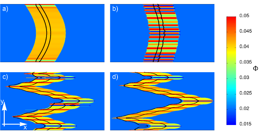
Figure 6: Moderate feedback corresponding to an effective curvature coefficient of $\tilde{\nu}=-1.059$ leads to V-shaped patterns moving much faster than a plane wave. Snapshots of a movie [31] for (a) $t=2$, (b) $t=7$, (c) $t=62$, and (d) $t=80$. Shown are clippings of size $30\times 30$ from a computational domain of size $110\times 30$, and feedback parameter values are $\Phi_{\text{min}}=0.018,\,\Phi_{\text{max}}=0.046$.

Originally, level set methods were developed by Osher and Sethian to compute and track the motion of interfaces. These methods have since been successfully applied in such diverse areas of applications as computer graphics, medical image segmentation and crystal growth [40, 41, 42].
We introduce a second field variable $\chi\left(\mathbf{r},\tau\right)$ which evolves in (virtual) time $\tau$ according to the so-called reinitialisation equation [43, 42, 44]

$$\partial_{\tau}\chi+\text{sign}\left(\chi^{0}\right)\left(\left|\nabla\chi\right|-1\right) = 0$$ (29)

with

$$\text{sign}\left(x\right)=\left\{\begin{array}[]{@{}l@{\quad}l}\hskip 8.53581pt1&\mbox{if $x>0$}\\ \hskip 8.53581pt0&\mbox{if $x=0$}\\ -1&\mbox{if $x<0$}\end{array}\right..$$ (30)

Equation (29) is solved with the initial condition

$$\chi\left(\mathbf{r},0\right) =\chi^{0}\left(\mathbf{r}\right)= u\left(\mathbf{r},t\right)-u_{c},$$ (31)

where $u_{c}$ is the activator value along the isoconcentration line $\boldsymbol{\gamma}$ for which we want to determine the curvature $\kappa$, i.e., $u\left(\boldsymbol{\gamma}\left(s,t\right),t\right)=u_{c}$. Note that $\chi\left(\boldsymbol{\gamma}\left(s,t\right),\tau\right)=\chi^{0}\left(\boldsymbol{\gamma}\left(s,t\right)\right)=0$ for all times $\tau$ such that the position of the level set $\boldsymbol{\gamma}$ is not changed by equation (29). However, equation (29) transforms the neighbourhood of $\chi=0$ such that, after sufficiently many time steps $\tau$,

$$\lim_{\tau\rightarrow\infty}\left|\nabla\chi\left(\mathbf{r},\tau\right)\right|=1.$$ (32)

The curvature $\kappa$ of $\boldsymbol{\gamma}$, equation(15) can now readily be computed in terms of the Laplacian of $\chi$ as

$$\kappa\left(s,t\right)=\tilde{\kappa}\left(\boldsymbol{\gamma}\left(s,t\right),t\right)=\lim_{\tau\rightarrow\infty}\Delta\chi\left(\boldsymbol{\gamma}\left(s,t\right),\tau\right).$$ (33)

Numerically, the evolution of $\chi$ up to the final time $\tau=0.01$ is sufficient to obtain a very accurate smooth result for the curvature of $\boldsymbol{\gamma}$. The reinitialisation equation (29) has to be solved at every real time step $t$. However, because the time evolution of the RD system is slow enough, we recompute the curvature $\kappa$ only every 200th time step $t$.

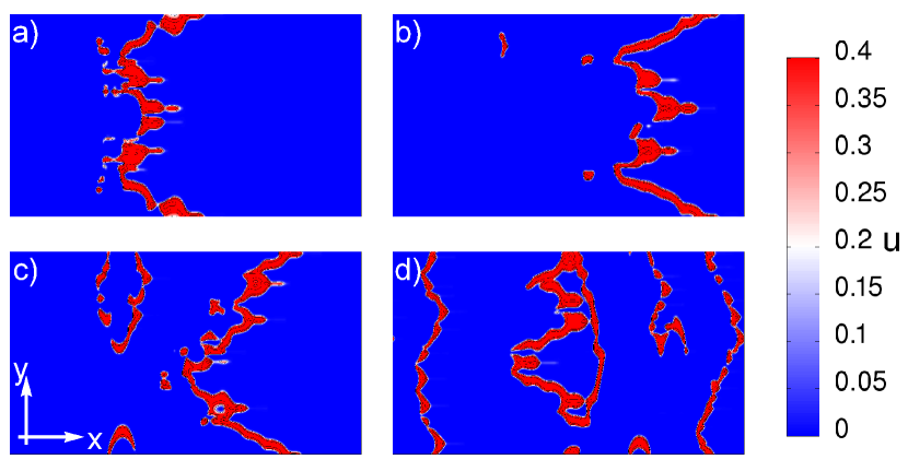
Figure 7: Segmentation of waves occurs under very strong feedback with an effective curvature coefficient of $\tilde{\nu}=-2.337$. Segments may break off, nucleate new waves and often start to rotate. Snapshots of a movie [31] for (a) $t=4$, (b) $t=6$, (c) $t=25$, and (d) $t=50$. The domain size is $110\times 30$, and feedback parameters are $\Phi_{\text{min}}=0.006,\,\Phi_{\text{max}}=0.05$.

3 Results

3.1 Excitation of transversal instabilities in the modified Oregonator model

We study the possibility to excite transversal instabilities by curvature-dependent feedback in the modified Oregonator model. The feedback law (24) is realised via the parameter $\Phi$ proportional to the illumination in the BZ reaction. For the parameters of the feedback law we set $\alpha=\Phi_{\text{max}}$ and $\beta=-\left(\Phi_{\text{max}}-\Phi_{\text{min}}\right)/\kappa_{\text{norm}}$ such that the effective curvature coefficient is

$$\tilde{\nu} = \nu-c_{1}\beta=\nu+\frac{c_{1}}{\kappa_{\text{norm}}}\left(\Phi_{\text{max}}-\Phi_{\text{min}}\right).$$ (34)

The values of $\Phi_{\text{max}}$ and $\Phi_{\text{min}}$ can be chosen arbitrarily as long as $\Phi_{\text{min}}<\Phi_{\text{max}}$ and both values lie in the regime of an excitable medium, see figure (4). The curvature $\kappa$ is determined for the activator isoconcentration line $\boldsymbol{\gamma}$ with $u\left(\boldsymbol{\gamma}\left(s,t\right),t\right)=u_{c}=0.2$. An area of fixed size in front of and behind $\boldsymbol{\gamma}$ is illuminated with the same value $\Phi\left(\kappa\left(s,t\right)\right)$, while within the remaining medium $\Phi$ attains its background value $\Phi=\Phi_{0}$. Before the feedback is switched on at time $t_{1}=0.4$, the wave evolves uncontrolled. The value of $\kappa_{\text{norm}}=1.2$ is an estimate of the largest value which the curvature attains during the overall time evolution. For simplicity, we choose a constant value of $\kappa_{\text{norm}}$, but in principle this value can be set to the maximum curvature every time the curvature is recomputed.
Figure 5 shows wave patterns arising for weak feedback with an effective curvature coefficient $\tilde{\nu}=-0.75$. The black solid lines denote the isoconcentration line $\boldsymbol{\gamma}$ for the activator level $u_{c}=0.2$. The rightmost line corresponds to the wave front while the trailing line corresponds to the wave back. The colours represent the value of the feedback parameter $\Phi$ and are proportional to the curvature of the wave front isoconcentration line. An initially sinusoidal shape decays and a plane wave with transversal modulations of small wavelength develops. For the example presented here, the modulations are not stationary but travel along the isoconcentration line until they annihilate each other or at the Neumann boundaries. For even weaker feedback, the modulations do not travel such that the pattern is truly stationary in a comoving frame of reference. The overall velocity of the patterns is approximately the velocity $c$ of the one-dimensional unperturbed traveling wave. Apart from the wave length of the modulations, this type of pattern appears similar to the patterns arising in the uncontrolled FHN model slightly beyond the threshold of transversal instabilities, see figure 1.

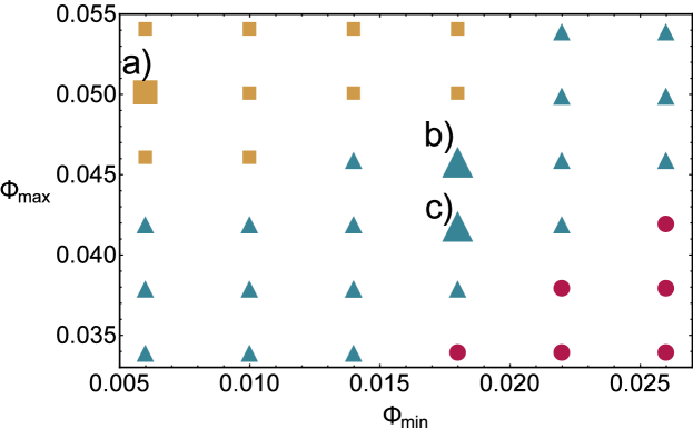
Figure 8: Phase diagram for patterns in the modified Oregonator model under feedback control. Blue bullets ${\color[rgb]{0.773,0.325,0.476}{\bullet}}$ correspond to folded waves stationary in a comoving frame of reference, green triangles ${\color[rgb]{0.423,0.643,0.698}{\blacktriangle}}$ stand for non-stationary wave front modulations, ochre squares ${\color[rgb]{0.860,0.709,0.470}{\blacksquare}}$ denotes segmentation of waves and spiral turbulence. a) refers to figure (7), b) to figure (6) and c) to figure (5).

Figure 6 displays the effects of moderate feedback with an effective curvature coefficient $\tilde{\nu}=-1.059$. V-shaped patterns arise which travel much faster than a corresponding one-dimensional solitary pulse. In a frame of reference comoving with the centre of mass, the V-shaped patterns appear stationary apart from modulations traveling along the isoconcentration line. The V-patterns observed under feedback are long-time stable and do not decay or break up. A solitary V-pattern in an unbounded domain can be explained analytically as a solution to the linear and nonlinear eikonal equations [45, 46]. A V with opening angle $\alpha$ has a mean velocity $V$ given by

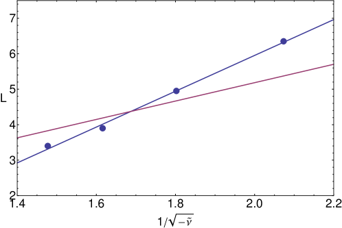
Figure 9: Transversal instabilities are suppressed in thin channels. Shown is the stability boundary of a plane wave under feedback in a channel of width $L$ with Neumann boundary conditions. Using feedback, the effective curvature coefficient $\tilde{\nu}=\nu-c_{1}\beta$ is adjusted until a plane wave becomes unstable. Red line: theoretical prediction equation (21) obtained from the Kuramoto-Sivashinsky equation. Blue dots: result of numerical simulations of the modified Oregonator model. Blue line: least square fit to numerical results.

$$V = \frac{c}{\sin\left(\alpha\right)},$$ (35)

where $c$ is the one-dimensional velocity. Because $\left|\sin\left(\alpha\right)\right|<1$, all V-patterns are moving faster than a plane wave. Experimentally, these patterns were observed in homogeneous [47] and stratified [48] BZ media.
Figure 7 shows the effect of strong feedback with an effective curvature coefficient $\tilde{\nu}=-2.337$. Similar as for moderate feedback, V-shaped patterns appear. However, their shape is non-stationary but oscillating. The V-shape is segmented in an irregular and non-stationary way, with segments either merging again or breaking off and serving as the nucleation centre for new waves. These new waves propagate as segmented circles and occasionally start to rotate until they annihilate upon collision with other waves. Qualitatively, the segmentation and occurrence of rotating segments is similar to the spreading spiral turbulence observed for the uncontrolled FHN model deep in the regime of transversal instabilities, see figure 2.
These results show that the proposed feedback law is not only able to excite transversal instabilities but allows, to some extent, the selection of the patterns beyond the instability threshold by tuning the feedback parameters $\Phi_{\text{max}}$ and $\Phi_{\text{min}}$ accessible to an experimenter. We display a phase diagram with a classification of the observed patterns in the $\Phi_{\text{max}}-\Phi_{\text{min}}$ plane in figure 8. Note that according to the KS equation (16), the observed patterns should only depend on the effective curvature coefficient $\tilde{\nu}$ given by equation (34). However, numerical simulations show that the type of patterns depends not only on the difference of $\Phi_{\text{max}}$ and $\Phi_{\text{min}}$, but also display a slight dependence on their absolute values. This dependence is due to nonlinear corrections in the relation for the one-dimensional velocity $c$ over $\Phi$ and higher order effects neglected by the KS equation (16).

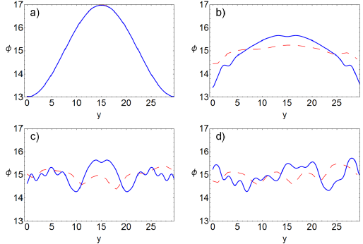
Figure 10: Time evolution of a wave’s isoconcentration line slightly beyond the threshold of transversal instability caused by feedback with an effective curvature coefficient $\tilde{\nu}=-0.02$. Compared are the results of two-dimensional numerical simulations of the modified Oregonator model (dotted red line) with the solution of the Kuramoto-Sivashinsky equation (blue line). Due to the strong dependence on the initial conditions, the time evolutions are comparable only for a short time span. (a) corresponds to $t=0$, (b) $t=6$, (c) $t=12$ and (d) $t=25$. Comparison is made in the comoving frame of reference because the centre of mass velocities do not agree.

By adjusting the effective curvature coefficient $\tilde{\nu}$, we are able to validate the predicted onset of transversal instabilities equation (21),

$$L=\frac{1}{\sqrt{-\tilde{\nu}}}\sqrt{\lambda}\pi$$ (36)

and its dependence on the channel width $L$. We perform numerical simulations of the controlled Oregonator model in a channel with width $L$ and Neumann boundary conditions in the $y$-direction. Starting with a plane box-like initial condition equation (10) with noisy box width $b$, we change the effective curvature coefficient $\tilde{\nu}$ until a plane wave becomes unstable, i.e., the curvature along the isoconcentration line is different from zero. Figure 9 shows that both numerical simulations and analytical prediction yield a linear relation between channel width $L$ and $1/\sqrt{-\tilde{\nu}}$ over a large range of effective curvature coefficients $\tilde{\nu}$. The slopes differ due to higher order corrections for the KS equation (16) and nonlinear corrections for the velocity $c$ over $\Phi$, equation (23), used for the feedback law.
Beyond the onset of transversal instabilities, the emerging patterns can in principle be described by the KS equation (16). We compare the time evolution of the modified Oregonator model with the solution of the KS equation for an effective curvature coefficient of $\tilde{\nu}=-0.02$. Because the centre of mass velocity is incorrectly predicted by the KS equation, figure 10 shows a sequence of snapshots of isoconcentration lines in a frame of reference comoving with the centre of mass. Due to the strong dependence on the initial data, any initial agreement between the two curves is vanishing fast during the time evolution.

3.2 Suppression of transversal instabilities

The curvature-dependent feedback law (24) is used to suppress transversal instabilities occurring in the uncontrolled piecewise linear FHN model given by equations (4), (5). Here, the excitation threshold $a$ is used as the feedback parameter. First, we linearly approximate the velocity - excitation threshold relation as

$$c\left(a\right) = c_{0}+c_{1}a,$$ (37)

with $c_{0}=2.23$ and $c_{1}=-8.75$. Similar as shown in figure (4) for the modified Oregonator model, solitary pulses exist only for a certain range of $a$ values. Second, the dependence of the excitation threshold $a$ on the curvature $\kappa$ is chosen as

$$a\left(\kappa\right) = \left\{\begin{array}[]{@{}l@{\quad}l}a_{\text{min}}+\beta\left(t\right)\kappa,&\kappa\geq 0,\\ a_{\text{min}}&\kappa<0.\end{array}\right.$$ (40)

The coefficient $\beta\left(t\right)$ is adjusted in time such that the maximum value of $a\left(\kappa\right)$ along the isoconcentration line does not exceed or undershoot the range of existence of solitary pulses. Every 100 time steps, we determine the maximum curvature $\kappa_{\text{max}}\left(t\right)$ along the isoconcentration line and set $\kappa_{\text{max}}$ to this value,

$$\beta\left(t\right) = \frac{a_{\text{max}}-a_{\text{min}}}{\kappa_{\text{max}}\left(t\right)}.$$ (41)

The background value of $a$ is set to $a_{0}=0.1$ everywhere before the feedback control is switched on at time $t=t_{1}=215$, and outside the region affected by the feedback control. Figure 11 displays the suppression of a transversal instability slightly beyond the threshold. For the same parameter values as in figure 1, the initially sinusoidally shaped wave relaxes back to a plane wave and no fold appears, see also the video in the supplemental material [31].

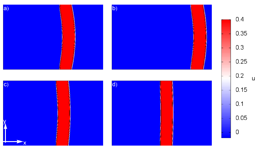
Figure 11: Curvature-dependent feedback control stabilises an unstable plane wave. For the same parameters slightly beyond the threshold of transversal instabilities as the corresponding uncontrolled time evolution in figure 1, the initially sinusoidally shaped wave relaxes back to a plane wave and no fold develops. Snapshots of a movie [31] with (a) $t=43$, (b) $t=67$, (c) $t=159$, and (d) $t=400$. The values of the feedback parameter are $a_{\text{min}}=0.05$ and $a_{\text{max}}=0.15$ and the control is switched on at $t=40$.

Patterns deep in the regime of transversal instabilities are characterised by a continuing segmentation of waves and spreading spiral turbulence as shown in figure 2. For the same parameter values, patterns stop to segment after the feedback is switched on, giving rise to a persistent plane wave and two counter rotating spiral waves, see figure 12. The wave front of rotating patterns has a nonbinding positive curvature. According to the linear eikonal equation (13), it advances slower than a plane wave if the effective curvature coefficient $\tilde{\nu}$ is positive. Therefore, the plane wave has a tendency to annihilate rotating waves, finally leading to a solitary plane wave.

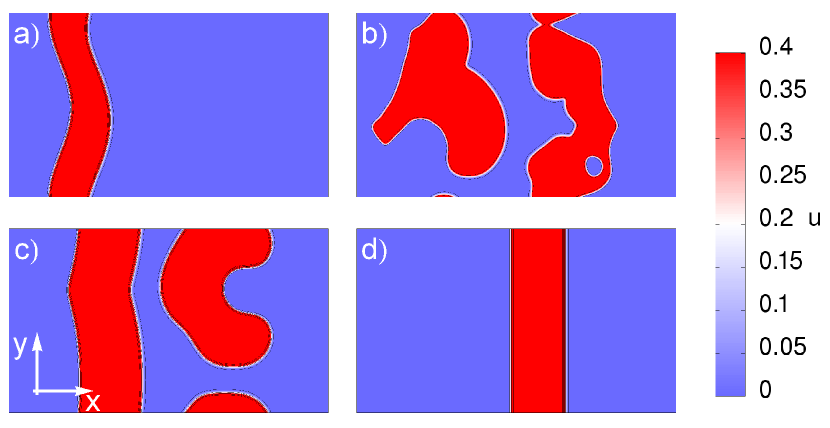
Figure 12: Curvature-dependent feedback suppresses spiral turbulence. After the feedback control is switched on at $t=256$ (b), waves stop to break up, leaving behind a plane wave and a pair of counter rotating spiral waves (c) and finally a solitary plane wave (d). Same parameters deep in the regime of transversal instabilities as the corresponding uncontrolled time evolution in figure 2. Snapshots of a movie [31] with (a) $t=5$, (b) $t=301$, (c) $t=672$, and (d) $t=891$. The values of the feedback parameter are $a_{\text{min}}=0.04$ and $a_{\text{max}}=0.08$.

4 Conclusions

In this article, we present a feedback loop to induce, control, and suppress transversal instabilities of reaction-diffusion waves. The control signal is calculated from the local curvature of the isoconcentration line of the wave. We show that the curvature dependent control can amplify or quench small curvature perturbations in the wave shape. Simultaneously, the feedback allows to study a large variety of artificially produced wave patterns associated with transversal instabilities. Often these patterns are non-stationary and sensitively depending on small changes in the initial conditions characteristic for chaotic dynamics.
Mathematically, the onset of transversal instabilities can be understood with the help of the linear eikonal equation which relates the wave velocity normal to an isoconcentration line to its local curvature. The coefficient $\nu$ in front of the curvature determines the stability of a flat wave. For positive values of $\nu$, convex wave segments slow down while concave wave segments propagate at a higher velocity. Under these conditions a perturbed flat traveling wave recovers its flat shape. In the case of negative $\nu$, a small positive curvature causes an increase of the wave velocity which in turn results in an increase of the local curvature. Now, a flat wave is unstable with respect to small curvature perturbations. The proposed feedback loop is able to change the sign of the coefficient $\nu$.
With experiments on chemical waves in the PBZR in mind, for realistic parameter values we show in numerical simulations with the Oregonator model that transversal instabilities of planar waves can be induced by the feedback. Right beyond the transversal instability of planar waves, we find nearly flat folded waves which are stationary in a comoving frame of reference. For weak feedback we observe small ripple-shaped undulations traveling along the wave front. Upon increasing the feedback strength further, V-shaped wave patterns with spatio-temporal transversal modulations appear. These V-shaped waves travel at a velocity that depends on the opening angle but is considerably faster than that of the planar wave. Far away from the instability threshold, breakup of waves causes persistent annihilation and merging of excited domains, self-sustained rotatory motion and nucleation of rotating wave segments. Qualitatively, the emerging wave patterns correspond to those observed in numerical simulations with separated activator and inhibitor diffusivity [11].
Regarding chemical wave propagation in the PBZR, we emphasise that the feedback parameters of the control law are experimentally accessible. For appropriate BZ recipes the dependence of the wave velocity on the intensity of applied light should be strong enough to induce transversal wave instabilities. The isoconcentration line of the wave can be determined by 2d spectrophotometry with sufficient spatial resolution using the contrast between the oxidised and reduced form of the catalyst. We believe that the computation of the curvature by the Level Set Method as described in Sec. 2.4 will work reliably for noisy experimental data, too. Because all chemical components share similarly shaped isoconcentration lines, the measurement of the concentration field of an arbitrary single chemical species is sufficient for setting up the control loop. Fine-tuning the feedback parameters allows to study the onset of transversal instabilities in dependence of the boundary conditions as e.g. the channel width $L$, as pointed out in chapter Sec. 2.2.
In the opposite case, sufficiently strong feedback changes the sign of the effective curvature coefficient from negative to positive. Consequently, naturally occurring transversal wave instabilities leading to the breakup of waves are suppressed - the feedback stabilises planar waves and spiral waves. Spreading of spiral turbulence is inhibited due to the suppression of segmentation of waves.
Reaction-diffusion waves describe, at least approximately, a huge variety of wave processes in biology. Our results are potentially applicable to deliberately induce or inhibit transversal wave instabilities and to control the emerging patterns under very general conditions. The essential condition for applicability is that the propagation velocity of the wave can be externally controlled over a sufficiently large range such that the curvature coefficient of the eikonal equation switches its sign.
Moreover, we expect that curvature dependent feedback might have interesting applications in interfacial pattern formation in general. For example, this feedback mechanism could be the starting point for a control strategy aimed at the purposeful selection of patterns affected by interfacial instabilities as, e.g., alloys growing into an undercooled melt.

Appendix A Parameter values for numerical simulations

parameter	value	description
$f$	$1.4$	stoichiometric parameter
$q$	$0.002$	system parameter
$1/\epsilon$	$49$	time scale separation
$1/\tilde{\epsilon}$	$4410$	time scale separation
$\Phi_{0}$	$0.02$	background illumination
$D_{u}$	$1.0$	activator diffusion coefficient
$D_{w}$	$1.2$	inhibitor diffusion coefficient
$\nu$	$1.05$	curvature coefficient
$\lambda$	$0.68$	fourth order coefficient in the KS equation
$c_{1}$	$-90.19$	slope of linear fit for velocity over $\Phi$
$c_{0}$	$9.01$	constant of linear fit for velocity over $\Phi$
$\kappa_{\text{norm}}$	$1.2$	curvature normalisation
$\Delta t$	$0.0001$	time step
$\Delta x$,$\Delta y$	$0.05$	step width of spatial resolution

Table 1: Parameter values used for numerical simulations of the modified Oregonator model.

parameter	value	description
$a$	$0.1$	excitation threshold
$k_{f}$	$2$	system parameter
$k_{g}$	$2$	system parameter
$\sigma$	$2.1$	ratio of diffusion coefficients
$\delta$	$0.01$	system parameter
$\epsilon$	$0.1575$	time scale separation
$c_{1}$	$-8.75$	slope of linear fit for velocity over $a$
$c_{0}$	$2.23$	constant of linear fit for velocity over $a$

Table 2: Parameter values used for numerical simulations of the piecewise linear FitzHugh-Nagumo model.

Appendix B Bonnet’s formula

We prove the formula of Bonnet, i.e., we demonstrate that evaluating the curvature field defined by equation (27) at an isoconcentration line $\boldsymbol{\gamma}$ yields the curvature of $\boldsymbol{\gamma}$.
Let $u=u\left(x,y\right)$ be the map $\mathbb{R}^{2}\rightarrow\mathbb{R}$ and $\boldsymbol{\gamma}\left(y\right)=\left(\gamma_{x}\left(y\right),y\right)^{T}$ be the isoconcentration line $\boldsymbol{\gamma}$ parametrised by $y$. It follows that $u\left(\gamma_{x}\left(y\right),y\right)=u_{c}=\text{const}.$ for all values of $y$. Therefore we can write (to shorten the notation, we write $\partial_{x}$u$\left(x,y\right)|_{x=\gamma_{x}\left(y\right)}$=$\partial_{x}$u$\left(\gamma_{x}\left(y\right),y\right)$)

$$\frac{d}{dy}u\left(\gamma_{x}\left(y\right),y\right) =\partial_{x}u\left(\gamma_{x}\left(y\right),y\right)\gamma_{x}^{\prime}\left(y\right)+\partial_{y}u\left(\gamma_{x}\left(y\right),y\right)= 0,$$ (42)

and

$$\frac{d^{2}}{dy^{2}}u\left(\gamma_{x}\left(y\right),y\right) = \frac{d}{dy}\left(\partial_{x}u\left(\gamma_{x}\left(y\right),y\right)\gamma_{x}^{\prime}\left(y\right)+\partial_{y}u\left(\gamma_{x}\left(y\right),y\right)\right)$$ (43)

$$= \partial_{x}u\left(\gamma_{x}\left(y\right),y\right)\gamma_{x}^{\prime\prime}\left(y\right)+\partial_{x}^{2}u\left(\gamma_{x}\left(y\right),y\right)\left(\gamma_{x}^{\prime}\left(y\right)\right)^{2}$$

$$+ 2\partial_{y}\partial_{x}u\left(\gamma_{x}\left(y\right),y\right)\gamma_{x}^{\prime}\left(y\right)+\partial_{y}^{2}u\left(\gamma_{x}\left(y\right),y\right)$$

$$= 0,$$

and generally $\frac{d^{n}}{dy^{n}}u\left(\gamma_{x}\left(y\right),y\right)=0$ with $n\in\mathbb{N},\,n>0$. The curvature field $\tilde{\kappa}$, Eq. (27), expressed in Cartesian coordinates is

$$\tilde{\kappa}\left(x,y\right)= \frac{\partial_{y}^{2}u\left(x,y\right)\left(\partial_{x}u\left(x,y\right)\right)^{2}-2\partial_{x}u\left(x,y\right)\partial_{y}u\left(x,y\right)\partial_{x,y}u\left(x,y\right)}{\left(\left(\partial_{x}u\left(x,y\right)\right)^{2}+\left(\partial_{y}u\left(x,y\right)\right)^{2}\right)^{3/2}}$$ (44)

$$+\frac{\partial_{x}^{2}u\left(x,y\right)\left(\partial_{y}u\left(x,y\right)\right)^{2}}{\left(\left(\partial_{x}u\left(x,y\right)\right)^{2}+\left(\partial_{y}u\left(x,y\right)\right)^{2}\right)^{3/2}}.$$

Evaluating $\tilde{\kappa}$ at the isoconcentration line yields

$$\tilde{\kappa}\left(\gamma_{x}\left(y\right),y\right)= \frac{\partial_{y}^{2}u\left(\gamma_{x}\left(y\right),y\right)\left(\partial_{x}u\left(\gamma_{x}\left(y\right),y\right)\right)^{2}+\partial_{x}^{2}u\left(\gamma_{x}\left(y\right),y\right)\left(\partial_{y}u\left(\gamma_{x}\left(y\right),y\right)\right)^{2}}{\left(\left(\partial_{x}u\left(\gamma_{x}\left(y\right),y\right)\right)^{2}+\left(\partial_{y}u\left(\gamma_{x}\left(y\right),y\right)\right)^{2}\right)^{3/2}}$$ (45)

$$-\frac{2\partial_{x}u\left(\gamma_{x}\left(y\right),y\right)\partial_{y}u\left(\gamma_{x}\left(y\right),y\right)\partial_{x,y}u\left(\gamma_{x}\left(y\right),y\right)}{\left(\left(\partial_{x}u\left(\gamma_{x}\left(y\right),y\right)\right)^{2}+\left(\partial_{y}u\left(\gamma_{x}\left(y\right),y\right)\right)^{2}\right)^{3/2}}.$$

Using Eq. (42), the denominator of Eq. (45) can be simplified as

$$\left(\partial_{x}u\left(\gamma_{x}\left(y\right),y\right)\right)^{2}+\left(\partial_{y}u\left(\gamma_{x}\left(y\right),y\right)\right)^{2} =\left(\partial_{x}u\left(\gamma_{x}\left(y\right),y\right)\right)^{2}+\left(-\partial_{x}u\left(\gamma_{x}\left(y\right),y\right)\gamma_{x}^{\prime}\left(y\right)\right)^{2}$$ (46)

$$=\left(\partial_{x}u\left(\gamma_{x}\left(y\right),y\right)\right)^{2}\left(1+\left(\gamma_{x}^{\prime}\left(y\right)\right)^{2}\right).$$

Similarly, using Eq. (42) and Eq. (43), the first term of the numerator of Eq. (45) can be rewritten in the form

$$\partial_{y}^{2}u\left(\gamma_{x}\left(y\right),y\right)\left(\partial_{x}u\left(\gamma_{x}\left(y\right),y\right)\right)^{2} = -\left(\partial_{x}u\left(\gamma_{x}\left(y\right),y\right)\right)^{2}\left(\vphantom{+\partial_{x}^{2}u\left(\gamma_{x}\left(y\right),y\right)\left(\gamma_{x}^{\prime}\left(x\right)\right)^{2}+2\partial_{x,y}u\left(\gamma_{x}\left(y\right),y\right)\gamma_{x}^{\prime}\left(y\right)}\partial_{x}u\left(\gamma_{x}\left(y\right),y\right)\gamma_{x}^{\prime\prime}\left(x\right)\right.$$

$$\left.+\partial_{x}^{2}u\left(\gamma_{x}\left(y\right),y\right)\left(\gamma_{x}^{\prime}\left(x\right)\right)^{2}+2\partial_{x,y}u\left(\gamma_{x}\left(y\right),y\right)\gamma_{x}^{\prime}\left(y\right)\right),$$

while the second term of the numerator of Eq. (45) can be cast as

$$\partial_{x}^{2}u\left(\gamma_{x}\left(y\right),y\right)\left(\partial_{y}u\left(\gamma_{x}\left(y\right),y\right)\right)^{2} = \partial_{x}^{2}u\left(\gamma_{x}\left(y\right),y\right)\left(\partial_{x}u\left(\gamma_{x}\left(y\right),y\right)\right)^{2}\left(\gamma_{x}^{\prime}\left(x\right)\right)^{2}.$$ (48)

The last term of the numerator of Eq. (45) becomes

$$-2\partial_{x}u\left(\gamma_{x}\left(y\right),y\right)\partial_{y}u\left(\gamma_{x}\left(y\right),y\right)\partial_{x,y}u\left(\gamma_{x}\left(y\right),y\right) =$$

$$2\left(\partial_{x}u\left(\gamma_{x}\left(y\right),y\right)\right)^{2}\partial_{x,y}u\left(\gamma_{x}\left(y\right),y\right)\gamma_{x}^{\prime}\left(y\right).$$ (49)

All terms except the term proportional to $\gamma_{x}^{\prime\prime}\left(x\right)$ in the numerator cancel. We are left with

$$\tilde{\kappa}\left(\gamma_{x}\left(y\right),y\right) = -\frac{\gamma_{x}^{\prime\prime}\left(y\right)}{\left(1+\left(\gamma_{x}^{\prime}\left(y\right)\right)^{2}\right)^{3/2}},$$ (50)

which is exactly the curvature of a graph, see Eq. (15).

References

References

- [1] J.S. Langer. Instabilities and pattern formation in crystal growth. Rev. Mod. Phys., 52(1):1, 1980.
- [2] E.A. Brener and V.I. Mel’Nikov. Pattern selection in two-dimensional dendritic growth. Adv. Phys., 40(1):53, 1991.
- [3] Philip Geoffrey Saffman and Geoffrey Taylor. The penetration of a fluid into a porous medium or hele-shaw cell containing a more viscous liquid. Proceedings of the Royal Society of London. Series A. Mathematical and Physical Sciences, 245(1242):312–329, 1958.
- [4] W. van Saarloos. Three basic issues concerning interface dynamics in nonequilibrium pattern formation. Phys. Rep., 301(1):9–43, 1998.
- [5] Anne De Wit and GM Homsy. Viscous fingering in reaction-diffusion systems. The Journal of chemical physics, 110(17):8663–8675, 1999.
- [6] G.I. Sivashinsky. Nonlinear analysis of hydrodynamic instability in laminar flames - I. derivation of basic equations. Acta Astronaut., 4(11):1177, 1977.
- [7] Ya B Zeldovich, GI Barenblatt, VB Librovich, and GM Makhviladze. The Mathematical Theory of Combustion and Explosions. Consultants Bureau, New York, 1985.
- [8] Rudolph V Birikh, Vladimir A Briskman, Manuel G Velarde, and Jean-Claude Legros. Liquid Interfacial Systems: Oscillations and Instability. CRC Press, 2003.
- [9] Elod Mehes and Tamas Vicsek. Collective motion of cells: from experiments to models. Integr. Biol., 6:831–854, 2014. URL: http://dx.doi.org/10.1039/C4IB00115J, doi:10.1039/C4IB00115J.
- [10] Athanasius FM Marée and Alexander V Panfilov. Spiral breakup in excitable tissue due to lateral instability. Physical review letters, 78(9):1819, 1997.
- [11] V.S. Zykov, A.S. Mikhailov, and S.C. Müller. Wave instabilities in excitable media with fast inhibitor diffusion. Phys. Rev. Lett., 81(13):2811, 1998.
- [12] Yoshiki Kuramoto. Chemical oscillations, waves, and turbulence. Courier Dover Publications, 2003.
- [13] Yoshiki Kuramoto. Instability and turbulence of wavefronts in reaction-diffusion systems. Progress of Theoretical Physics, 63(6):1885–1903, 1980. doi:10.1143/PTP.63.1885.
- [14] D. Horváth, V. Petrov, S.K. Scott, and K. Showalter. Instabilities in propagating reaction-diffusion fronts. J. Chem. Phys., 98(8):6632, 1993.
- [15] D. Horváth and K. Showalter. Instabilities in propagating reaction-diffusion fronts of the iodate-arsenous acid reaction. J. Chem. Phys., 102:2471, 1995.
- [16] D. Horváth and Á. Tóth. Diffusion-driven front instabilities in the chlorite–tetrathionate reaction. J. Chem. Phys., 108:1447, 1998.
- [17] Vladimir K. Vanag and Irving R. Epstein. Pattern formation in a tunable medium: The belousov-zhabotinsky reaction in an aerosol ot microemulsion. Phys. Rev. Lett., 87:228301, Nov 2001. URL: http://link.aps.org/doi/10.1103/PhysRevLett.87.228301, doi:10.1103/PhysRevLett.87.228301.
- [18] V.K. Vanag and I.R. Epstein. Segmented spiral waves in a reaction-diffusion system. Proc. Natl. Acad. Sci. U.S.A., 100(25):14635, 2003.
- [19] D. Horváth, Á. T., and K. Yoshikawa. Electric field induced lateral instability in a simple autocatalytic front. J. Chem. Phys., 111:10, 1999.
- [20] A. Tóth, D. Horváth, and W. van Saarloos. Lateral instabilities of cubic autocatalytic reaction fronts in a constant electric field. J. Chem. Phys., 111:10964, 1999.
- [21] Ágota Tóth, Dezsö Horváth, Éva Jakab, John H Merkin, and Stephen K Scott. Lateral instabilities in cubic autocatalytic reaction fronts: the effect of autocatalyst decay. J. Chem. Phys., 114:9947, 2001.
- [22] Eugene Mihaliuk, Tatsunari Sakurai, Florin Chirila, and Kenneth Showalter. Feedback stabilization of unstable propagating waves. Phys. Rev. E, 65:065602, Jun 2002. doi:10.1103/PhysRevE.65.065602.
- [23] T. Sakurai, E. Mihaliuk, F. Chirila, and K. Showalter. Design and control of wave propagation patterns in excitable media. Science, 296(5575):2009–2012, 2002. doi:10.1126/science.1071265.
- [24] O. Steinbock, V. Zykov, and S.C. Müller. Control of spiral-wave dynamics in active media by periodic modulation of excitability. Nature, 366(6453):322–324, 1993. doi:10.1038/366322a0.
- [25] Vladimir S. Zykov, Oliver Steinbock, and Stefan C. Müller. External forcing of spiral waves. Chaos, 4(3):509–518, 1994. doi:10.1063/1.166029.
- [26] V. S. Zykov, G. Bordiougov, H. Brandtstädter, I. Gerdes, and H. Engel. Global control of spiral wave dynamics in an excitable domain of circular and elliptical shape. Phys. Rev. Lett., 92:018304, Jan 2004. doi:10.1103/PhysRevLett.92.018304.
- [27] J. Schlesner, V. Zykov, H. Engel, and E. Schöll. Stabilization of unstable rigid rotation of spiral waves in excitable media. Phys. Rev. E, 74:046215, Oct 2006. doi:10.1103/PhysRevE.74.046215.
- [28] J Schlesner, VS Zykov, H Brandtstädter, I Gerdes, and H Engel. Efficient control of spiral wave location in an excitable medium with localized heterogeneities. New J. Phys., 10(1):015003, 2008. doi:10.1088/1367-2630/10/1/015003.
- [29] H. J. Krug, L. Pohlmann, and L. Kuhnert. Analysis of the modified complete oregonator accounting for oxygen sensitivity and photosensitivity of Belousov-Zhabotinskii systems. J. Phys. Chem., 94(12):4862, 1990.
- [30] V.S. Zykov. Simulation of Wave Processes in Excitable Media. Manchester University Press, 1987.
- [31] See Supplemental Material at [URL will be inserted by publisher] for movies.
- [32] H. Dierckx, O. Bernus, and H. Verschelde. Accurate eikonal-curvature relation for wave fronts in locally anisotropic reaction-diffusion systems. Phys. Rev. Lett., 107(10):108101, 2011.
- [33] V.S. Zykov. Biophysics (USSR), 25:906, 1980.
- [34] A.S. Mikhailov and V.S. Zykov. Kinematical theory of spiral waves in excitable media: Comparison with numerical simulations. Physica D: Nonlinear Phenomena, 52:379 – 397, 1991. doi:http://dx.doi.org/10.1016/0167-2789(91)90134-U.
- [35] V.S. Zykov and H. Engel. Feedback-mediated control of spiral waves. Physica D, 199(12):243, 2004. doi:10.1016/j.physd.2004.10.001.
- [36] A. Malevanets, A. Careta, and R. Kapral. Biscale chaos in propagating fronts. Phys. Rev. E, 52(5):4724, 1995.
- [37] Y. Kuramoto. Diffusion-induced chaos in reaction systems. Prog. Theor. Phys. Supp., 64:346, 1978.
- [38] P. Cvitanović, R. Artuso, R. Mainieri, G. Tanner, and G. Vattay. Chaos: Classical and Quantum. Niels Bohr Institute, Copenhagen, 2012. ChaosBook.org.
- [39] Elsa Abbena, Simon Salamon, and Alfred Gray. Modern differential geometry of curves and surfaces with Mathematica. CRC press, third edition, 2006.
- [40] S. Osher and J.A. Sethian. Fronts propagating with curvature-dependent speed: Algorithms based on Hamilton-Jacobi formulations. J. Comput. Phys., 79(1):12 – 49, 1988.
- [41] J.A. Sethian. Level Set Methods and Fast Marching Methods: Evolving Interfaces in Computational Geometry, Fluid Mechanics, Computer Vision, and Materials Science, volume 3. Cambridge University Press, 1999.
- [42] S. Osher and R. Fedkiw. Level Set Methods and Dynamic Implicit Surfaces, volume 153. Springer, 2003.
- [43] G. Russo and P. Smereka. A remark on computing distance functions. J. Comput. Phys., 163(1):51, 2000.
- [44] A. du Chéné, C. Min, and F. Gibou. Second-order accurate computation of curvatures in a level set framework using novel high-order reinitialization schemes. J. Sci. Comput., 35(2-3):114–131, 2008.
- [45] Pavel K. Brazhnik and Vasily A. Davydov. Non-spiral autowave structures in unrestricted excitable media. Physics Letters A, 199(1):40 – 44, 1995. doi:http://dx.doi.org/10.1016/0375-9601(95)00024-W.
- [46] Pavel K. Brazhnik. Exact solutions for the kinematic model of autowaves in two-dimensional excitable media. Physica D, 94(4):205 – 220, 1996. doi:http://dx.doi.org/10.1016/0167-2789(96)00042-5.
- [47] V. Pérez-Muñuzuri, M. Gómez-Gesteira, A. P. Muñuzuri, V. A. Davydov, and V. Pérez-Villar. -shaped stable nonspiral patterns. Phys. Rev. E, 51:R845–R847, Feb 1995. URL: http://link.aps.org/doi/10.1103/PhysRevE.51.R845, doi:10.1103/PhysRevE.51.R845.
- [48] O. Steinbock, V. S. Zykov, and S. C. Müller. Wave propagation in an excitable medium along a line of a velocity jump. Phys. Rev. E, 48:3295–3298, Nov 1993. URL: http://link.aps.org/doi/10.1103/PhysRevE.48.3295, doi:10.1103/PhysRevE.48.3295.