Nonlinearity and nonclassicality in a nanomechanical resonator

Abstract

We address quantitatively the relationship between the nonlinearity of a mechanical resonator and the nonclassicality of its ground state. In particular, we analyze the nonclassical properties of the nonlinear Duffing oscillator (being driven or not) as a paradigmatic example of a nonlinear nanomechanical resonator. We first discuss how to quantify the nonlinearity of this system and then show that the nonclassicality of the ground state, as measured by the volume occupied by the negative part of the Wigner function, monotonically increases with the nonlinearity in all the working regimes addressed in our study. Our results show quantitatively that nonlinearity is a resource to create nonclassical states in mechanical systems.

I Introduction

Mechanical systems are emerging as very well suited candidates for the study of quantum behavior at the mesoscopic scale. Such a possibility is currently being explored in particular in the domain of quantum opto-/electro-mechanics Aspelmeyer , where ground-breaking experimental demonstration of quantum control of massive systems operating under explicitly adverse conditions have been recently made Rogers . Yet, despite the substantial number of studies addressing the features of mechanical systems operating at the quantum level, only partial attention has so far been given to the physics of nonlinear mechanical devices. Classically, it is known that many nonlinear systems exhibit very complex behaviors of potentially interesting features holmes , and it is currently believed that such features might be potentially useful in many areas of investigation, even beyond physics.

In the context of mesoscopic quantum behaviors, Katz et al. have studied the quantum-to-classical transition in the state of nonlinear nanoelectromechanical systems (NEMS) katz . Their analysis considered both an isolated resonator and one open to the effects of an environment, focusing on quantum signatures and on their disappearance toward classicality, as the operating temperature of the oscillator was raised.

In this paper, we study the link between the enforcement of nonlinearity in a quantum mechanical oscillator and the manifestation of evidently nonclassical features in its state. Wondering about such a connection is indeed significant: the expectation values taken by observables of linear systems follow the corresponding classical equations of motion, and a linear dynamics do not let phase-space non-classicality emerge (even at low temperatures). It is thus important, and relevant for applications, to understand which is the interplay between the nonlinear character of the evolution of a given bosonic system and the strength of the nonclassical features that we are able to correspondingly enforce.

From a quantitative viewpoint, here we will make use of the negativity of the Wigner function as a phase-space indicator of nonclassicality ana . This is an established notion of nonclassicality, with a close relationship with the non-local properties of the quantum state coh97 ; ban98 . On the other hand, we will quantify the degree of nonlinearity of a given system by making use of the measures put forward by some of us in Ref. paris14 . In order to complement the analysis presented in Ref. katz , we focus on the case of Duffing-type nonlinearity which, besides being technologically relevant as inherent in some forms of NEMS postma , has been the focus of a few studies on the quantum effects that it entails in terms of non-classicality Duffing_NCl and entanglement Duffing_Ent . We show that a direct link exists between nonlinearity and the nonclassical character of the state of the oscillator. By focusing explicitly on the ground state of the system, we show that the phase-space nonclassicality of such state depends almost linearly on the degree of nonlinearity of the oscillator, thus suggesting a potential role of the latter feature as a resource for the achievement of strong quantumness. Our conclusions are valid for a driven and an undriven Duffing oscillator, thus covering a vast range of physically relevant situations. We believe that our analysis and results embody a first interesting step towards the establishment of a rigorous link between such fundamental features in the dynamics of an oscillator.

The remainder of the paper is structured as follows. In Sec. II we discuss the specific example of nonlinear oscillator, a Duffing oscillator, considered in this work. We focus on the undriven configuration of such oscillator and introduce the relevant measures of nonlinearity and nonclassicality that will be used throughout the paper. We show that a direct correspondence between degree of nonlinearity and nonclassicality can be established, pointing at the relevance of former for the enforcement of the latter in the ground state of an oscillator. Sec. III deals with the case of a driven Duffing oscillator, and reports an analysis similar to the one presented in Sec. II. We show that the relation between measures of nonlinearity and non classicality is maintained in a dynamical situation as well, thus highlighting the fundamental nature of the relationship that we find, which appears to be unrelated to the details of the working conditions of the oscillator. Finally, Sec. IV closes the paper with some concluding remarks.

II Nonlinearity of a Duffing oscillator: Undriven case

We consider a Duffing oscillator, which is described by the Hamiltonian Carr

$$\hat{H}_{sys}=\frac{1}{2}(\hat{p}^{2}+\hat{x}^{2})+\frac{1}{4}\varepsilon\hat{x}^{4}-\hat{x}{\cal F}\cos\omega t,$$ (1)

where $\hat{x}$ and $\hat{p}$ are the dimensionless position- and momentum-like operators of the oscillator (such that $[\hat{x},\hat{p}]=i$), $\varepsilon$ is the anharmonicity parameter, ${\cal F}$ is the amplitude of a possible force that drives the oscillator at frequency $\omega$. Without loss of generality, throughout the manuscript we will consider the case of a stiffening nonlinearity with $\varepsilon>0$. Such model is appropriate to describe the energy of a small-size doubly clamped mechanical resonator such as a carbon nanotube, or a nanowire postma . The onset of nonlinear effects in such systems decreases with decreasing diameter of the device, making either weak driving forces or thermomechanical noise sufficient to drive the motion away from the linear approximation. In this Section we will focus on the undriven case, thereby setting ${\cal F}=0$, deferring the treatment of a driven one to the next Section.

It is instructive to gather an understanding of the form of the nonlinear potential energy to which the oscillator is subjected. In the left panel of Fig. 1 we show the function $V(x)=\varepsilon x^{4}/4$ for different choices of the anharmonicity parameter, which shows that an increasing value of $\varepsilon$ results in more pronounced nonlinear effects at smaller displacements from the equilibrium position $x=0$ of the oscillator. The effects of the quartic potential on the wave functions of the oscillator can be evaluated by using time-independent perturbation theory. In such context, we use the notation $\hat{H}_{sys}=\hat{H}^{(0)}+\hat{V}(\hat{x})$ with

$$\hat{H}^{(0)}=\frac{1}{2}(\hat{x}^{2}+\hat{p}^{2}),\qquad\hat{V}(\hat{x})=\frac{1}{4}\varepsilon\hat{x}^{4}.$$ (2)

We thus evaluate the first-order corrections to the eigenstates $\{\left|n\right\rangle\}$ of $\hat{H}^{(0)}$ as

$$|\psi_{n}\rangle\approx|n\rangle+\sum_{k\neq n}\frac{\langle k|\hat{V}(\hat{x})|n\rangle}{n-k}|k\rangle.$$ (3)

We will mostly focus on the ground state (GS) of the nonlinear oscillator, for which we aim at finding an approximate form. While a fully numerical approach could be used to gather the full form of the GS of the oscillator, the range of values that $\varepsilon$ can take experimentally well justifies a perturbative approach. The perturbing Hamiltonian only couples $|0\rangle$ to $|2\rangle$ and $|4\rangle$, so that we have the normalised approximation of the GS

$$|\psi_{0}\rangle={\cal N}\left[|0\rangle-\frac{3\varepsilon}{8\sqrt{2}}|2\rangle-\frac{\sqrt{3}\varepsilon}{16\sqrt{2}}|4\rangle\right]$$ (4)

with ${\cal N}=1/\sqrt{1+\frac{39\varepsilon^{2}}{512}}$. The corresponding probability densities are plotted on the right panel of Fig. 1 for increasing values of $\varepsilon$, showing how the nonlinear term in the potential tends to localize the wave function of the oscillator around its equilibrium position.

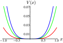
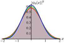
Figure 1: (Color online) The Duffing potential. In the left panel we show $V(x)$ for $\varepsilon=0.2$ (red), $\varepsilon=0.5$ (green), $\varepsilon=0.8$ (blue). In the right panel we show the corresponding GS probability densities, $|\psi_{0}|^{2}(x)$.

In order to determine the range of values of $\varepsilon$ within which the form of $\left|\psi_{0}\right\rangle$ given in Eq. (4) holds, we have calculated numerically the GS $\left|\psi_{num}\right\rangle$ of the Hamiltonian $\hat{H}_{sys}$ in Eq. (2) using a truncated Hilbert space consisting of the first 51 number states and evaluated the state fidelity $F(\varepsilon)=|\langle\psi_{0}|\psi_{num}\rangle|^{2}$, whose behavior against the nonlinearity parameter $\varepsilon$ is shown in Fig. 2. Fidelity remains above $95\%$ for $\varepsilon\in[0,0.8]$. All the results reported in the remainder of this paper have been gathered using this range of values. As we show now, both the information on the modified potential energy and the GS wave function are key for the analysis at the core of this paper.

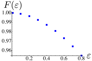
Figure 2: (Color online) State fidelity $F(\varepsilon)$ between the ground state of the undriven Duffing oscillator achieved through a perturbative approach $\left|\psi_{0}\right\rangle$ and that estimated numerically by diagonalising the Hamiltonian model in Eq. (2) using the first 51 number states.

We now pass to the introduction of the quantitative tools that we plan to adopt in order to gather insight into the relation between nonlinearity and the onset of non classicality in the Duffing oscillator at hand. We would like to stress that the figures of merit that we introduce here go beyond the mere quantification of nonlinearity as given by the Hamiltonian parameters (e.g., as given by $\epsilon$ itself). This has the twofold advantage of allowing to encompass situations in which more than one Hamiltonian parameter is considered (see next Section) and of removing the dependence on the detailed form of the non-linear potential.

We first consider a measure of nonlinearity based on the features of the GS paris14 and built by comparing $|\psi_{0}\rangle$ and its unperturbed counterpart $|0\rangle$. Quantitatively, we determine the distance between the two GSs using the Bures measure: Given a perturbing nonlinear potential $\hat{V}(\hat{x})$, we define the nonlinearity measure $\eta_{\text{B}}\left[V\right]$ as the suitably normalized Bures distance $D_{\scriptscriptstyle B}$ between the GS of the oscillator under consideration and that of the corresponding harmonic one. In our case, we have

$$\eta_{\scriptscriptstyle B}\left[\hbox{V}\right]=\frac{1}{\sqrt{2}}\,D_{\scriptscriptstyle B}\left[|\psi_{0}\rangle,|0\rangle\right]=\sqrt{1-|{}\langle 0\left|\psi_{0}\rangle\right|},$$ (5)

where we have used the fact that the two states under scrutiny are pure. As it is apparent from its very definition, this quantifier depends crucially upon the choice of a corresponding reference harmonic potential. Such a dependence can be overcome by considering a second way of quantifying nonlinearity: Given a potential $\hat{V}(\hat{x})$ with associated GS $\left|0\right\rangle_{V}$, we define the measure of nonlinearity $\eta_{\scriptscriptstyle N\!G}\left[\hbox{V}\right]$

$$\eta_{\scriptscriptstyle N\!G}\left[\hbox{V}\right]=\delta_{\scriptscriptstyle N\!G}\left[|0\rangle\langle 0|_{\scriptscriptstyle V}\right],$$ (6)

where $\delta_{\scriptscriptstyle N\!G}[\varrho]$ is the degree of non-Gaussianity introduced in Ref. ng2 ; ng3 . This definition is intuitive: as commented earlier, a nonlinear potential would induce deviations from Gaussianity, which can in turn be used to quantify the strength of the nonlinear process itself. The degree of non-Gaussianity is built on the quantum relative entropy of the state and a reference Gaussian state. As the GSs under scrutiny are always pure, we have

$$\eta_{\text{NG}}\left[\hbox{V}\right]=S[\tau]=h\left(\sqrt{\hbox{det}[{\boldsymbol{\sigma}}_{\tau}]}\right)$$ (7)

with $\tau$ the reference Gaussian state, $S[\tau]$ its Von Neumann entropy, $\boldsymbol{\sigma}_{\tau}$ its covariance matrix, and $h(x)=(x+\frac{1}{2})\ln(x+\frac{1}{2})-(x-\frac{1}{2})\ln(x-\frac{1}{2})$. The crucial point here is that the definition of $\eta_{\text{NG}}$ requires the determination of a reference Gaussian state for the GS of $V(x)$ rather than a reference harmonic potential for $V(x)$ itself. Both measures are zero for a harmonic potential, whereas they may lead to different definitions of maximally nonlinear processes.

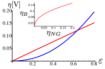
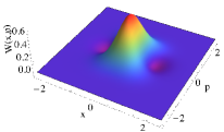
Figure 3: (Color online) Left: the nonlinearity measures $\eta_{\scriptscriptstyle B}\left[\text{V}\right]$ (red line) and $\eta_{\scriptscriptstyle N\!G}\left[\text{V}\right]$ (blue line) for the undriven oscillator as a function of $\varepsilon$. The inset is a parametric plot of $\eta_{\scriptscriptstyle B}$ as a function of $\eta_{\scriptscriptstyle N\!G}$, showing that the two measures are monotone functions of each other. The right panel shows the Wigner function of the GS for $\varepsilon=0.1$

While $0\leq\eta_{B}[\hbox{V}]\leq 1$, the upper bound being reached if and only if the external potential $\hat{V}(\hat{x})$ gives rise to a GS orthogonal to that of the corresponding harmonic case, $\eta_{\text{NG}}$ is unbound from above, which complicates the quantitative comparison between the two figures of merit. A suitable rescaling can be obtained at any fixed value of energy upon normalizing $\eta_{\text{NG}}$ to the degree of non-Gaussianity of the states that achieve maximal non-Gaussian character at that value of the energy. This class includes number states and some specific superposition of them (see ng3 for details). The maximum of this rescaled quantity is thus achieved for a potential having a GS equal to a number state ($n\neq 0$) of the harmonic oscillator or to some specific superpositions of them.

One would expect that the nonlinearity increases with $\varepsilon$. Indeed, as shown in Fig. 3, this intuitive behaviour is captured by both measures, $\eta_{\text{NG}}\left[\hbox{V}\right]$ and $\eta_{\text{B}}\left[\hbox{V}\right]$, which grow continuously and smoothly with $\varepsilon$. The two measure are also linked by a monotonic relationship. This is demonstrated in the inset of Fig. 3, where we show a parametric plot of $\eta_{\scriptscriptstyle B}\left[\hbox{V}\right]$ against $\eta_{\scriptscriptstyle N\!G}\left[\hbox{V}\right]$, the curvilinear abscissa in such plot being embodied by $\varepsilon$. Numerically, for $\varepsilon\in[0,0.8]$, the relation between the two measures of nonlinearity is very well approximated by the function

$$\eta_{B}[\hbox{V}]=a+b\sqrt{\eta_{NG}[\hbox{V}]}$$ (8)

with $a\simeq 2.7\times 10^{-3}$ and $b\simeq 0.34$.

A broadly used indicator of nonclassicality in the state of an oscillator is provided by the volume occupied by its associated Wigner function in the negative region of the phase space ana . The Wigner function of the state $\rho$ of a single oscillator system is defined as

$$W_{\rho}(\alpha)=\frac{1}{\pi}\int e^{\alpha\xi^{*}-\alpha^{*}\xi}\chi_{\rho}(\xi)d^{2}\xi,$$ (9)

where $\chi_{\rho}(\xi)={\rm Tr}[\rho e^{\xi\hat{a}^{\dagger}-\xi^{*}\hat{a}}]$ is the Weyl characteristic function and $\xi,\alpha\in{\mathbb{C}}$. Unlike a true probability distribution, the Wigner function can take on negative values wig ; wig84 ; cah , which is a striking signature of nonclassicality. In the right panel of Fig. 3 we show the Wigner function of the GS of the Duffing oscillator, showing the presence of regions of negativity that signal the nonclassical nature of the state of the system. In order to quantify such nonclassicality we use the measure

$$\nu(\rho)=\frac{\eta_{\rho}}{1+\eta_{\rho}}$$ (10)

with $\eta(\rho)=\int_{-\infty}^{\infty}|W_{\rho}(\alpha)|d^{2}\alpha-1$ the negative volume of the Wigner function. The quantity $\eta(\rho)$, which is per se sufficient to characterize phase-space nonclassicality, has been employed to study the quantum-to-classical transition in both linear and nonlinear oscillators katz ; kleckner , as well as to characterize the performance of conditional schemes for the preparation of nonclassical states of massive oscillators Rogers ; paternostroPRL . Here we consider its rescaled version according to Eq. (10), which provides a number $\nu(\rho)\in[0,1]$ that is thus amenable to a quantitative comparison with the proposed measures of nonlinearity.

Making use of Eq.  (9) for the Wigner function of the GS of the Duffing resonator, we can evaluate the measure of nonclassicality through a numerical integration. In Fig. 4 we show the plot of the NG-based nonlinearity measure $\eta_{\scriptscriptstyle N\!G}$ against the normalized measure of nonclassicality $\nu(\psi_{0})$. A numerical nonlinear fit gives the functional relation

$$\eta_{NG}=0.002+0.207\sqrt{\nu(\psi_{0})}+2.731\nu(\psi_{0}),$$ (11)

showing that after an initial trait, the link between the two quantities becomes linear, ensuring the proportionality of the two figures of merit under scrutiny.

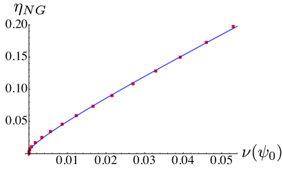
Figure 4: (Color online) We plot the the nonlinearity measure $\eta_{\scriptscriptstyle N\!G}\left[\text{V}\right]$ against the normalized measure of $\nu(\psi_{0})$ nonclassicality based on the negative parts of the Wigner-function for the GS of the undriven Duffing resonator. We show that the two measures are monotone functions of each other. The squares show the values of $\eta_{NG}$ at set nonclassicality of the ground state of the undriven Duffing oscillator. The solid line represents the fit given by Eq. (11). After an initial trait where $\eta_{NG}$ grows as $\sqrt{\nu(\psi_{0})}$, the relation between the two figures of merit becomes approximately linear, showing the direct connection between nonlinearity and nonclassical character of the state of the oscillator.

III Nonlinearity of a Duffing oscillator: driven case

We shall now pass to the analysis of a driven Duffing resonator, which is an example of nonlinear resonator often encountered in relevant experimental situations craig ; postma ; kozinsky ; aldridge . The dimensionless Hamiltonian of the system is thus Eq. (1) with the explicit inclusion of the time-dependent driving term $-\hat{x}{\cal F}\cos\omega t$. In what follows, we choose a working point well within the region of bistability of the oscillator (which is ensured for ${\cal F}\in[0.015,0.06]$ and $\omega\in[1.016,1.02]$). The form of the driving potential ${\hat{V}}^{d}(\hat{x},t)=\frac{1}{4}\varepsilon\hat{x}^{4}-\hat{x}{\cal F}\cos\omega t$ is illustrated in Fig. 5, showing the deformation induced by the nonlinear and time-dependent part of the perturbation.

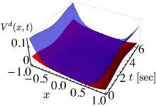
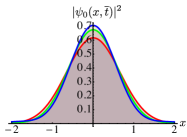
Figure 5: (Color online) In the left panel we show $V^{d}(x,t)$ against time and position for ${\cal F}=0.015$, $\varepsilon=0.1$ (red, opaque surface), and $\varepsilon=0.5$ (blue, transparent surface). In the right panel we show the corresponding GS probability densities, $|\psi_{0}(x,\overline{t}=1)|^{2}$ for the same set of parameters.

In order to evaluate the form of the GS associated with the full model, we shall resort to the use of time-dependent perturbation theory. We decompose the state of the system at $t=0$, when the perturbative potential is off, as

$$|\psi(0)\rangle=\sum_{n}c_{n}{(0)}|n\rangle~{}~{}~{}(c_{n}(t)\in{\mathbb{C}})$$ (12)

and aim at finding a perturbative expansion $c^{(q)}_{n}(t>0)\in{\mathbb{C}}$ at order $q\in{\mathbb{Z}}$ in the perturbation, so that the state of the system at the corresponding order becomes

$$|\psi^{(q)}(t)\rangle\simeq\sum_{n}c^{(q)}_{n}(t)e^{iE_{n}t/\hbar}|n\rangle,$$ (13)

where $E_{n}$ is the eigenvalue of the unperturbed Hamiltonian corresponding to the eigenstates $\left|n\right\rangle$. The first-order correction in both ${\cal F}$ and ${\varepsilon}$, which will be the highest order of the perturbative expansion that we will consider here, is given by sak

$$c^{(1)}_{n}(t)=-{i}\int_{0}^{t}e^{i\omega_{n\ell}t^{\prime}}V^{d}_{nl}(t^{\prime})dt^{\prime},$$ (14)

with $c^{(0)}_{n}(t)=\delta_{nl}$, $V^{d}_{nl}(t)=\langle n|\hat{V}^{d}(\hat{x},t)|l\rangle$ and $e^{i(E_{n}-E_{l})t}=e^{i\omega_{nl}t}$. The explicit calculation of $|\psi(t)\rangle$ up to the stated order of approximation and for $|\psi(0)\rangle=|{0}\rangle$ leads us to the GS wavefunction

$$\psi_{0} (x,t)={\cal M}\left\{\bigg{(}1-\frac{3it\varepsilon}{16}\bigg{)}e^{-it/2}\psi_{0}(x)\right.$$

$$+ {\cal F}\,\frac{(1-e^{it}[\cos\omega t-i\omega\sin\omega t])}{\sqrt{2}(\omega^{2}-1)}e^{-3it/2}\psi_{1}(x)$$

$$+ \frac{\varepsilon}{16}\!\Bigg{[}{3\sqrt{2}(e^{-5it/2}-e^{-it/2})}\psi_{2}(x)$$

$$\qquad{+}\frac{(e^{-\frac{9}{2}it}-e^{-\frac{i}{2}t})}{4}\psi_{4}(x)\Bigg{]}\Bigg{\}}$$

being ${\cal M}$ the normalisation factor and $\psi_{n}(x)\equiv\langle x|n\rangle$ the wave function of state $|n\rangle$. A plot of the spatial distribution $|\psi_{0}(x,\overline{t})|^{2}$ at a set time $\overline{t}$ is shown in the right panel Fig. 5.

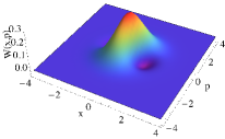
Figure 6: (Color online) Left: the nonlinearity measures $\eta_{\scriptscriptstyle B}\left[\text{V}\right]$ (red line) and $\eta_{\scriptscriptstyle N\!G}\left[\text{V}\right]$ (blue line) for the driven oscillator as a function of $\varepsilon$ and for the choice of parameters ${\cal F}=0.015$, $t=1$ and $\omega=1.018$ which ensures that the resonator is in the bistability region. The inset is a parametric plot of $\eta_{\scriptscriptstyle B}$ as a function of $\eta_{\scriptscriptstyle N\!G}$, showing that the two measures are monotone functions of each other. The right panel shows the Wigner function for the same set of parameters and $\varepsilon=0.1$.

Looking at the potential, one would expect that the nonlinearity increases with $\varepsilon$ at any fixed values of the given parameters. Indeed, this intuitive behavior is captured by both measures, $\eta_{\scriptscriptstyle N\!G}\left[\text{V}\right]$ and $\eta_{\scriptscriptstyle B}\left[\text{V}\right]$, as they grow continuously. The two measures are monotonic functions of each other, as illustrated in the left panel of Fig. 6. In the right panel we also show the Wigner function for $t=1$, which shows negative regions and thus the signature of nonclassicality. When assessed against the chosen indicator of nonclassicality, $\eta_{NG}$ is again found to be in direct correspondence with the volume occupied by the Wigner function corresponding to $|\psi_{0}(t)\rangle$ [cf. Fig. 7].

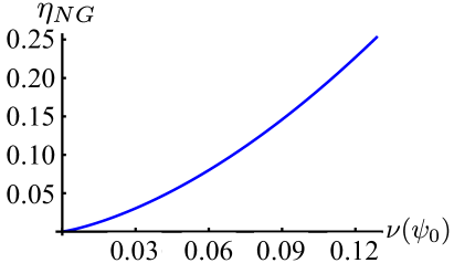
Figure 7: (Color online) A parametric plot of the normalized measure of $\nu(\psi_{0})$ nonclassicality based on the negative parts of the Wigner-function for the GS of the driven Duffing resonator as a function of the nonlinearity measure $\eta_{\scriptscriptstyle N\!G}\left[\text{V}\right]$ (parameters $\varepsilon=0.01$, $t=1$, $\omega=1.018$, and ${\cal F}=0.015$) appears to be roughly linear and monotonically increasing.

IV Conclusions

In this paper, upon using purpose-tailored quantitative figures of merit, we have addressed in some details the relation between nonlinearity and nonclassicality in a class of nonlinear oscillators that is relevant in many contexts, including experimental solid state physics. By approximating the form of the ground state of the oscillator through a perturbative approach (either stationary or time-dependent) we have been able to demonstrate that the negativity of Wigner function, which is a well-acquired measure of nonclassicality in continuous variable systems, is in monotonic relation with recently proposed measures of nonlinearity, therefore reinforcing the idea of nonlinearity as a catalyst of quantumness. Although our conclusions have been gathered by addressing the specific example of a Duffing oscillator, our work paves the way to interesting extensions, primarily concerned with the application of our tools to other forms of nonlinearities tocome .

A second interesting direction of investigation would deal with the inclusion of environmental effects, and with the possibility to shield the degree of nonclassicality enforced in the state of a quantum oscillator through a suitable degree of nonlinearity. This might entail an interesting way of protecting quantumness, stemming from the direct, non-demanding control of the Hamiltonian of the oscillator. In fact, while the harmonic assumption is an approximation valid within many contexts (from nano-mechanical oscillators to ultracold atomic systems in external potential), switching to explicitly non-harmonic situations is typically straightforward by the means of a strong driving. This is generally more economic than time-gated external pulses (required in dome of the techniques devised so far for the protection of quantum features) or the control of the properties of the environment, which is typically of not easy access. Work along these lines is in progress and results will be presented elsewhere.

References

- (1) M. Aspelmeyer, T. J. Kippenberg, and F. Marquardt, arXiv:1303.0733 (2013).
- (2) B. Rogers, N. Lo Gullo, G. De Chiara, G. M. Palma, and M. Paternostro, Quantum Meas. Quantum Metr. 2, 11 (2014).
- (3) J. Guckenheimer, P. Holmes, Nonlinear Oscillations, Dynamical Systems, and Bifurcations of Vector Fields, (Springer, New York, 1983).
- (4) I. Katz, A. Retzker, R. Straub, and R. Lifshitz, Phys. Rev. Lett. 99, 040404 (2007); I. Katz, R. Lifshitz, A. Retzker, and R. Straub, New J. Phys. 10 125023 (2008).
- (5) A. Kenfack and K. Zyckowski, J. Opt. B 6, 396 (2004).
- (6) O. Cohen, Phys. Rev. A 56, 3484 (1997).
- (7) K. Banaszek, K. Wodkiewicz, Phys. Rev. A 58, 4345 (1998).
- (8) M. G. A. Paris, M. G. Genoni, N. Shammah, and B. Teklu, Phys. Rev. A 90, 012104 (2014).
- (9) H.W. C. Postma, I. Kozinsky, A. Husain, and M. L. Roukes, Appl. Phys. Lett. 86, 223105 (2005); V. Peano and M. Thorwart, New J. Phys. 8, 21 (2006).
- (10) A. Kolkiran and G.S. Agarwal arXiv:cond-mat/0608621 (2006); S. Rips, M. Kiffner, I. Wilson-Rae and M.J. Hartmann, New J. Phys. 14 023042 (2012); X.Y. Lü, J.Q. Liao, L. Tian, and F. Nori, arXiv:1403.0049 (2014).
- (11) C. Joshi, M. Jonson, E. Andersson, and P. Ohberg, J. Phys. B: At. Mol. Opt. Phys. 44, 245503 (2011); S. Rips and M.J. Hartmann, Phys. Rev. Lett. 110, 120503 (2013); V. Montenegro, A. Ferraro, and S. Bose, Phys. Rev. A 90, 013829 (2014).
- (12) S. M. Carr, W. E. Lawrence and M. N. Wybourne, Phys. Rev. B64, 220101 (R) (2001).
- (13) M. G. Genoni, M. G. A. Paris, K. Banaszek, Phys. Rev. A 78 , 060303(R) (2008).
- (14) M. G. Genoni, M. G. A. Paris, Phys. Rev. A 82, 052341 (2010).
- (15) E. Wigner, Phys. Rev. 40, 749 (1932).
- (16) M. Hillery, R. F. O’Connell, M. O. Scully, and E. P. Wigner, Phys. Rep. 106, 121 (1984).
- (17) K. E. Cahill, R. J. Glauber, Phys. Rev. 177, 1882 (1969)
- (18) D. Kleckner, I. Pikowski, E. Jeffrey, L. Ament, E. Eliel, J. van der Brink, and D. Bouwmeester, New. J. Phys. 10, 095020 (2008).
- (19) M. Paternostro, Phys. Rev. Lett. 106, 183601 (2011); J. Li, S. Gröblacher, and M. Paternostro, New. J. Phys. 15, 033023 (2013).
- (20) H. G. Craighead, Science 290, 1532 (2000).
- (21) I. Kozinsky, H.W.C. Postma, I. Bargatin, and M. L. Roukes, Appl. Phys. Lett. 88, 253101 (2006).
- (22) J. S. Aldridge and A. N. Cleland, Phys. Rev. Lett. 94,156403 (2005).
- (23) J. J. Sakurai, Modern Quantum Mechanics, Revised Edition, Addison-Wesley (1994).
- (24) F. Albarelli, A. Ferraro, M. Paternostro, M. G. A. Paris, in preparation