First moment of the flavour octet nucleon parton distribution function using lattice QCD

Abstract

We perform a lattice computation of the flavour octet contribution to the average quark momentum in a nucleon, $\langle x\rangle^{(8)}_{\mu^{2}=4~{}\mathrm{GeV}^{2}}$. In particular, we fully take the disconnected contributions into account in our analysis for which we use a generalization of the technique developed in Dinter:2012tt . We investigate systematic effects with a particular emphasis on the excited states contamination. We find that in the renormalization free ratio $\frac{\langle x\rangle^{(3)}}{\langle x\rangle^{(8)}}$ (with $\langle x\rangle^{(3)}$ the non-singlet moment) the excited state contributions cancel to a large extend making this ratio a promising candidate for a comparison to phenomenological analyses. Our final result for this ratio is in agreement with the phenomenological value and we find, including systematic errors, $\frac{\langle x\rangle^{(3)}}{\langle x\rangle^{(8)}}=0.39(1)(4)$.

1 Introduction

Computing nucleon properties from first principles using lattice QCD is a long standing challenge. In particular, moments of parton distribution functions (pdfs) are important benchmark quantities for lattice calculations and provide insight into the structure of hadrons. The computation of various moments of pdfs is therefore a very active research area for lattice calculations, see Alexandrou:2013joa ; Alexandrou:2011nr ; Alexandrou:2011db ; Alexandrou:2010hf ; Bali:2013dpa ; Bali:2012av ; Green:2012ud ; Hagler:2007xi ; Alexandrou:2013cda ; Constantinou:2014tga for recent results. In the work we perform here a first lattice calculation of the octet contribution to the average quark momentum in a nucleon, $\langle x\rangle^{(8)}_{\mu^{2}}$ is presented, where $\mu^{2}$ denotes the renormalization scale. This quantity is of interest by itself and can be extracted from phenomenological analyses of data from deep inelastic scattering experiments, see below. It therefore can serve as an additional quantity to probe QCD and the structure of hadrons, see Constantinou:2014tga .

In addition, $\langle x\rangle^{(8)}_{\mu^{2}}$ needs the same renormalization constant as the iso-vector averaged quark momentum in the nucleon $\langle x\rangle^{(3)}_{\mu^{2}}$ and therefore in the ratio of $\langle x\rangle^{(8)}_{\mu^{2}}$ and $\langle x\rangle^{(3)}_{\mu^{2}}$ the renormalization constant cancels. Although we can evaluate non-perturbatively the renormalization constant, its cancelation in the ratio eliminates any uncertainty related to its determination. Comparing the ratio to a phenomenological analysis can thus help to understand, whether renormalization effects can play a role in the presently observed discrepancy between lattice calculations of $\langle x\rangle^{(3)}_{\mu^{2}}$ and phenomenological determinations of this quantity.

Despite the above given motivations to compute $\langle x\rangle^{(8)}_{\mu^{2}}$ there is so far no value of this quantity available from a lattice determination. The reason for this is that $\langle x\rangle^{(8)}_{\mu^{2}}$ is very difficult to calculate since it involves dis-connected, singlet contributions. The definition of the flavour octet moment $\langle x\rangle^{(8)}_{\mu^{2}}$ reads :

$$\langle x\rangle^{(8)}_{\mu^{2}}=\int_{-1}^{1}dx~{}x\left[u(x,\mu^{2})+d(x,\mu^{2})-2s(x,\mu^{2}))\right]$$ (1)

where $q(x,\mu)$ denotes the sum of the parton distribution function of the quark $q$ and anti-quark $\bar{q}$. Using the same convention, we also define the non-singlet contribution $\langle x\rangle^{(3)}_{\mu^{2}}$,

$$\langle x\rangle^{(3)}_{\mu^{2}}=\int_{-1}^{1}dx~{}x\left[u(x,\mu^{2})-d(x,\mu^{2})\right]\;.$$ (2)

At a value of the renormalization scale of $\mu^{2}=4{\rm GeV}^{2}$ the two moments$\langle x\rangle^{(3)}_{\mu^{2}=4~{}\mathrm{GeV}^{2}}$ and $\langle x\rangle^{(8)}_{\mu^{2}=4~{}\mathrm{GeV}^{2}}$ can be extracted phenomenologically using parton distribution functions determined from deep inelastic scattering data, and read, using the ABM12 pdfs set Alekhin:2013nda and the analysis of ref. Sergey

$$\langle x\rangle^{(3)}_{\mu^{2}=4~{}\mathrm{GeV}^{2}}=0.153(4),\hskip 10.0pt\langle x\rangle^{(8)}_{\mu^{2}=4~{}\mathrm{GeV}^{2}}=0.470(7).$$ (3)

The quantities $\langle x\rangle^{(3)}_{\mu^{2}}$ and $\langle x\rangle^{(8)}_{\mu^{2}}$ are related to matrix elements of local operators that can be computed in Euclidean space-time and are hence accessible to lattice QCD calculations. Introducing

$$O^{a}_{\{\mu_{1}\cdots\mu_{n}\}}=\overline{\psi}\gamma_{\{\mu_{1}}i\overleftrightarrow{D}_{\mu_{2}}\cdots i\overleftrightarrow{D}_{\mu_{n}\}}\lambda^{a}\psi\\$$ (4)

where $\lambda^{a}$ are the Gell-Mann matrices acting on a three flavour quark field $\psi=(u,d,s)$. With $\overleftrightarrow{D}$ we denote the symmetrized covariant lattice derivative and with the curly brackets the symmetrization and subtraction of the trace. The required matrix element is then given by

$$\langle N(p,s)|O^{a=3,8}_{\{\mu\nu\}}|N(p,s)\rangle\lvert_{\mu^{2}}=\langle x\rangle^{(3,8)}_{\mu^{2}}\bar{u}_{N}(p,s)\gamma_{\{\mu}P_{\nu\}}u_{N}(p,s)\;.$$ (5)

From the definition in eq. (1) it is clear that the octet matrix element $\langle N(p,s)|O^{a=8}_{\{\mu\nu\}}|N(p,s)\rangle$ involves dis-connected contributions which have in general a bad signal to noise ratio, require thus a very high statistics and are consequently very difficult to compute on the lattice. In addition, the dis-connected contribution to $\langle x\rangle^{(8)}_{\mu^{2}}$ is an $SU(3)_{\rm flavour}$ breaking effect and is thus expected to be small. In Dinter:2012tt and Alexandrou:2013wca we have demonstrated that for the here used (maximally) twisted mass lattice discretization of QCD there are special noise reduction techniques which can help substantially to improve on the signal to noise ratio. Indeed, these techniques allowed us to compute a number of quantities which were very difficult to access before Alexandrou:2013nda ; Abdel-Rehim:2013wlz .

In this work we present a generalization of the particular technique used in the context of the determination of the $\sigma$-terms Dinter:2012tt to calculate non-perturbatively the disconnected contribution relevant for $\langle x\rangle^{(8)}_{\mu^{2}}$. As we will see below, this generalization will indeed provide a statistically significant signal for $\langle x\rangle^{(8)}_{\mu^{2}}$. Note that contrary to the case of the $\sigma$-terms, the formalism to compute dis-connected contributions developed here is not limited to the twisted mass formulation. The technique could also be applied to other flavour octet operators which would allow to determine non perturbatively moments of polarized pdfs or the flavour octet axial coupling of the nucleon $g_{A}^{(8)}$ for instance, see e.g. Alexandrou:2013wca ; Abdel-Rehim:2013wlz .

The paper is organized as follow : after describing the basic ingredients of our computation we give the details of the variance reduction technique used in this work. We then present a study of the systematic effects appearing in our calculation and perform an extrapolation of the results to the physical pion mass in order to compare with the phenomenologically obtained values.

2 Simulation Details

The lattice action used in our simulations includes as active degrees of freedom, besides the gluon field, a mass-degenerate light up and down quark doublet as well as a strange-charm quark pair in the sea, a situation which we refer to as the $N_{f}=2+1+1$ setup. We use the Iwasaki action Iwasaki:1985we for the pure gauge action and the twisted mass fermion formulation for the Dirac action. In particular, we make use of the formulation of refs.  Frezzotti:2000nk ; Frezzotti:2003ni for the light mass degenerate $u$–$d$ sector, while the action introduced in refs. Frezzotti:2003xj ; Frezzotti:2004wz is employed for the mass non-degenerate $c$–$s$ sector. The quark mass parameters of the heavy flavour pair have been tuned so that in the unitary lattice setup the Kaon and D-meson masses, take approximately their experimental values. More information about the $N_{f}=2+1+1$ setup scheme and further simulation details can be found in ref. Baron:2010bv ; Baron:2010th . For the results we will show here, we have employed two values of the lattice spacing determined using the nucleon mass in Alexandrou:2013joa . They read $a\approx 0.082~{}\mathrm{fm}$ ($\beta=1.95$) and $a\approx 0.064~{}\mathrm{fm}$ ($\beta=2.1$). In addition, we will use a number of quark masses corresponding to pion masses in the range of $300~{}\mathrm{MeV}-500~{}\mathrm{MeV}$. The parameters of the ensembles used in this work are summarized in Table 1.

label	$\beta$	$a\,\mu_{l}$	Volume	$m_{\rm{PS}}~{}[MeV]$
B35.32	1.95	0.0035	32${}^{3}\times$64	302
B55.32	1.95	0.0055	32${}^{3}\times$64	372
B75.32	1.95	0.0075	32${}^{3}\times$64	432
B85.24	1.95	0.0085	24${}^{3}\times$48	466
D45.32sc	2.1	0.0045	32${}^{3}\times$64	372

Table 1: Ensembles used in this work and relevant parameters.

In order to fix the notation, we introduce the twisted mass lattice Dirac operator $D_{f,\rm tm}$ for a doublet of mass degenerate quarks :

$$D_{f,\rm tm}[U]=D_{\rm W}[U]+ia\mu_{f}\gamma_{5}\tau^{3}\;.$$ (6)

Here $D_{\rm W}[U]$ is the Wilson Dirac operator, $\mu_{f}$ denotes the bare twisted mass and $\tau^{3}$ is the third Pauli matrix. For further needs we also introduce the operators $D_{f,\pm}$ denoting the upper and lower flavour components of $D_{f,\rm tm}[U]$, referred to as the Osterwalder-Seiler (OS) lattice Dirac operator:

$$D_{f,\pm}[U]=\rm{tr}~{}\left\{\frac{1\pm\tau_{3}}{2}D_{f,\rm tm}[U]\right\},$$ (7)

where $\rm{tr}$ denotes the trace in flavour space. We will call $D_{f,\pm}[U]$ the lattice Dirac operator of an Osterwalder-Seiler quark with mass $\pm\mu_{f}$.

When we discuss below the 2-point and 3-point correlation functions necessary for this work, we will use the so-called physical basis of quark fields denoted as $\psi_{f}$. The physical field basis is related to the twisted quark field basis, $\chi_{f}$, by the following field rotation,

$$\psi_{f}\equiv e^{i\frac{\omega_{f}}{2}\gamma_{5}\tau^{3}}\chi_{f}\hskip 10.0pt\textmd{and}\hskip 10.0pt\overline{\psi}_{f}\equiv\overline{\chi}_{f}e^{i\frac{\omega_{f}}{2}\gamma_{5}\tau^{3}},$$ (8)

where the twist angle $\omega_{f}=\pi/2$ at maximal twist. In addition, $\psi_{f}$ with index $f=l,s$ will denote quark field doublets of light ($l$) or strange ($s$) quarks depending on the mass $\mu_{f}$ chosen in the valence sector. Since $\psi_{f}$ will always refer to the physical basis we will denote with $u$ and $d$ the two components of $\psi_{l}$. Following the notation of Eq. (7) we will denote with $s_{\pm}$ the two components of $\psi_{s}$. Employing the OS Dirac operator in the valence sector for the strange quark leads to a mixed action where the strange OS quark mass has been tuned to match within errors the unitary Kaon mass.

2.1 Nucleon matrix elements

The nucleon two-point function is defined in the physical basis by

$$C^{\pm}_{N,\rm 2pts}(t)=\sum_{\vec{x}}\rm{tr}~{}\Gamma^{\pm}\langle{\mathcal{J}}_{N}(x)\overline{{\mathcal{J}}}_{N}(0)\rangle,$$ (9)

where the source position is fixed to 0 in order to lighten notations and $t$ thus denotes the source-sink separation. We also introduced the parity projectors $\Gamma^{\pm}=(1\pm\gamma_{0})/{2}$. The subscript $N$ refers to the proton or to the neutron state for which the standard interpolating fields are given by the formulae:

$${\mathcal{J}}_{p}=\epsilon^{abc}\left(u^{a,T}{\mathcal{C}}\gamma_{5}d^{b}\right)u^{c}\hskip 10.0pt\textmd{and}\hskip 10.0pt{\mathcal{J}}_{n}=\epsilon^{abc}\left(d^{a,T}{\mathcal{C}}\gamma_{5}u^{b}\right)d^{c}.$$ (10)

Note that using discrete symmetries and anti-periodic boundary conditions in the time direction for the quark fields, one can show that $C^{+}_{N,\rm 2pts}(t)=-C^{-}_{N,\rm 2pts}(T-t)$. Let us also recall that an exact symmetry of the action leads to the following relation at a finite value of lattice spacing, $C^{\pm}_{n,\rm 2pts}(t)=C^{\pm}_{p,\rm 2pts}(t)$ Alexandrou:2008tn . In order to improve the overlap between the ground state and the interpolating fields of the nucleon we use Gaussian smearing of the quark fields appearing in the interpolating fields. We also use APE smearing of the gauge links involved in the Gaussian smearing.

The nucleon three-point functions is given by

$$C^{\pm,a}_{N,\rm 3pts}(t_{s},t_{\rm{op}})=\sum_{\vec{x_{\rm s}},\vec{x}_{\rm op}}\rm{tr}~{}\Gamma^{\pm}\langle{\mathcal{J}}_{N}(x_{\rm s})O^{a=3,8}_{\{44\}}(x_{\rm op})\overline{{\mathcal{J}}_{N}}(0)\rangle,$$ (11)

where $O^{a=3,8}_{\{44\}}$ is one of the twist-2 operators introduced in Eq. (4), $t_{\rm op}$ is the time of insertion of the operator, and $t_{s}$ denotes the so-called source-sink separation. Note that the precise definition of the strange quark field entering in the operator $O^{a=8}_{\{44\}}$ is postponed to the next subsection.

Using the two- and three-point correlators of Eqs. (9) and (11), we construct the following ratio:

$$R^{a}(t_{s},t_{\rm op})\equiv\frac{C^{+,a}_{N,\rm 3pts}(t_{s},t_{\rm op})}{am_{N}C^{+}_{N,\rm 2pts}(t_{s})}=\langle x\rangle^{(a)}_{\rm bare}+{\mathcal{O}}(e^{-\Delta Mt_{\rm op}})+{\mathcal{O}}(e^{-\Delta M(t_{s}-t_{\rm op})}),$$ (12)

where $am_{N}$ is the nucleon mass in lattice units and $\Delta M$ is the mass gap between the lowest nucleon state and the first excited state with the same quantum numbers. One can thus extract from the asymptotic time behaviour of $R^{a=8}(t_{s},t_{\rm op})$ the bare quantity $\langle x\rangle^{(8)}_{\rm bare}$ and correspondingly $\langle x\rangle^{(3)}_{\rm bare}$.

2.2 Lattice evaluation

While the light quark fields used in the operator $O^{a=3,8}_{\{44\}}$ are the unitary fields we use, as mentioned already above, a different action for the valence strange quark. In practice we introduce a doublet of mass degenerate quarks with a mass $a\mu_{s}$ tuned to reproduce the unitary Kaon mass. This procedure introduces an error due to the uncertainty on the determination of the matching mass that we will discuss later on but will allow us to use an efficient noise reduction technique that will be explained in the next section.

Consider the following operator in terms of the field in the twisted mass basis :

$$J^{8}=\overline{\chi}\gamma_{\{4}i\overleftrightarrow{D}_{4\}}\chi-\bar{\chi}_{s}\gamma_{\{4}i\overleftrightarrow{D}_{4\}}\chi_{s}$$ (13)

Performing the rotation to the physical basis, we obtain :

$$J^{8}=\overline{\psi}\gamma_{\{4}i\overleftrightarrow{D}_{4\}}\psi-\bar{\psi}_{s}\gamma_{\{4}i\overleftrightarrow{D}_{4\}}\psi_{s}=\bar{u}\gamma_{\{4}i\overleftrightarrow{D}_{4\}}u+\bar{d}\gamma_{\{4}i\overleftrightarrow{D}_{4\}}d-\bar{s}_{+}\gamma_{\{4}i\overleftrightarrow{D}_{4\}}s_{+}-\bar{s}_{-}\gamma_{\{4}i\overleftrightarrow{D}_{4\}}s_{-}$$ (14)

Note that $J^{8}$ keeps the same form in the two bases and that $J^{8}$ is only one possible choice for a discretization of the operator $O^{a=8}_{\{44\}}$. While the two-point nucleon correlators of Eq. (9) give only rise to quark-connected Wick contractions, in general the three-point functions of Eq. (11) yield both quark-connected (illustrated in Fig. 1a) and quark-disconnected (illustrated in Fig. 1b) contributions. In the following we will refer to them simply as to connected and disconnected fermionic Wick contractions (or diagrams) and shall write

$$C^{\pm,a}_{N,\rm 3pts}(t_{s},t_{\rm{op}})=\widetilde{C}^{\pm,a}_{N,\rm 3pts}(t_{s},t_{\rm{op}})+{\mathcal{D}}^{\pm,a}_{N,\rm 3pt}(t_{s},t_{\rm{op}})$$ (15)

with $\widetilde{C}^{\pm,a}_{N,\rm 3pt}$ (resp. ${\mathcal{D}}^{\pm,a}_{N,\rm 3pt}$) corresponding to the connected (resp. disconnected) quark diagrams, defined as

$$\widetilde{C}^{\pm,a}_{N,\rm 3pt}(t_{s},t_{\rm{op}})=\!\sum_{\vec{x},\,\vec{x}_{\rm op}}{\rm{tr}}~{}\left\{\Gamma^{\pm}\langle\big{[}{\mathcal{J}}_{N}(x)O^{a}_{\{44\}}(x_{\rm op})\overline{{\mathcal{J}}_{N}}(x_{\rm src})\big{]}\rangle\right\}\,,$$ (16)

$${\mathcal{D}}^{\pm,a}_{N,\rm 3pt}(t_{s},t_{\rm{op}})=\!\sum_{\vec{x},\,\vec{x}_{\rm op}}{\rm{tr}}~{}\left\{\Gamma^{\pm}\langle\big{[}{\mathcal{J}}_{N}(x)\overline{{\mathcal{J}}_{N}}(x_{\rm src})\big{]}\big{[}O^{a}_{\{44\}}(x_{\rm op})\big{]}\rangle\right\}\,,$$ (17)

where the symbol $[...]$ is a shorthand for all the connected fermionic Wick contractions. Note that for $a=3$, the disconnected part is a ${\mathcal{O}}(a^{2})$ effect which vanishes in the continuum limit and can thus be neglected. Introducing

$$\delta_{\pm}^{(\mu,\mu_{s})}(t_{\rm op})=\sum_{\vec{x}_{\rm op}}{\rm{tr}}~{}~{}\left\{\left(\frac{1}{D_{l,\pm}[U]}-\frac{1}{D_{s,\pm}[U]}\right)_{(x_{\rm op},x_{\rm op})}~{}\right\}\,,$$ (18)

the contribution of the disconnected fermion loop to ${\mathcal{D}}^{\pm,a}_{N,\rm 3pt}$ on a given gauge configuration $U$ in our setup reads

$${\mathcal{D}}^{\pm,a}_{N,\rm 3pt}(t_{s},t_{\rm{op}})=\langle C^{\pm}_{N,\rm 2pts}(t_{s})\left(\delta_{+}^{(\mu,\mu_{s})}(t_{\rm op})+\delta_{-}^{(\mu,\mu_{s})}(t_{\rm op})\right)\rangle,$$ (19)

The connected contributions $\widetilde{C}^{\pm,a}_{N,\rm 3pt}(t_{s},t_{\rm{op}})$ have been evaluated using standard techniques for three-point functions (sequential inversions through the sink), see e.g. ref. Alexandrou:2013joa .

 

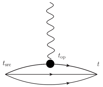
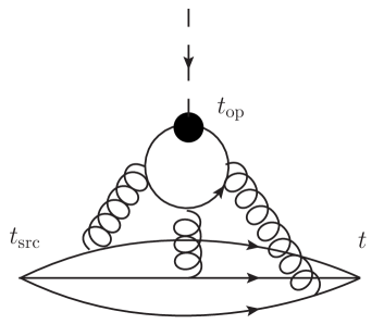
Figure 1: Connected (left) and the disconnected (right) graphs arising from the Wick contractions of the here considered 3-point functions.

2.3 Estimation of disconnected loops

We describe here the generalization of the variance reduction method for twisted mass fermions introduced and discussed in  Michael:2007vn ; Boucaud:2008xu ; Dinter:2012tt ; Alexandrou:2013wca .

Consider the identity

$$D_{l,\pm}-D_{s,\pm}=\pm i\gamma_{5}a\left(\mu_{l}-\mu_{s}\right)$$ (20)

implying that

$$\frac{1}{D_{l,\pm}}-\frac{1}{D_{s,\pm}}=-\frac{1}{D_{s,\pm}}\left(D_{l,\pm}-D_{s,\pm}\right)\frac{1}{D_{l,\pm}}=\mp ia\left(\mu_{l}-\mu_{s}\right)\frac{1}{D_{s,\pm}}\gamma_{5}\frac{1}{D_{l,\pm}},$$ (21)

where we have used Eq. (20) to obtain the last equality.

For the practical calculation, we introduce a set $\Xi$ of $N_{\xi}$ independent random volume sources, $\{\xi_{[1]},\dots,\xi_{[r]},\dots,\xi_{[N_{\xi}]}\}$, satisfying

$$\lim_{N_{\xi}\to\infty}\left[\xi^{i}_{[r]}(x)^{\ast}\xi^{j}_{[r]}(y)\right]_{\Xi}=\delta_{xy}\delta^{ij}$$ (22)

where $i=1,...,12$ refers to the spin and color indices of the source and $[\dots]_{\Xi}$ denotes the average over the $N_{\xi}$ noise sources in $\Xi$ .

Applying $O^{a}_{\{44\}}$ to Eq. (21) and taking the trace over spin and colour indices we obtain :

$$\mp ia\left(\mu_{l}-\mu_{s}\right)\sum_{\vec{x}}\left[\phi_{[r],l,\mp}^{*}\gamma_{5}O^{a}_{\{44\}}\phi_{[r],s,\pm}(x)\right]_{R}=\delta_{\pm}^{(\mu,\mu_{s})}(t_{\rm op})+{\mathcal{O}}\left(R^{-1/2}\right),$$ (23)

where

$$\phi_{[r],s,\pm}=(1/D_{s,\pm})\xi_{[r]}\hskip 10.0pt\textmd{and}\hskip 10.0pt\phi_{[r],l,\pm}^{*}=\xi_{[r]}^{*}(1/D_{l,\pm})^{{\dagger}}.$$ (24)

For the generation of the random sources we have used a $\mathbf{Z}_{2}$ noise taking all field components randomly from the set $\{1,-1\}$.

Note that $\delta_{\pm}^{(\mu,\mu_{s})}$, and by construction its variance, is proportional to the mass difference $\mu_{l}-\mu_{s}$ and vanishes on each configuration in the limit $\mu_{s}\to\mu_{l}$. Our approach, thus, exactly encodes the fact that the disconnected contributions we are interested in vanish in the $SU(3)_{\rm flavour}$ limit.

2.4 Renormalization

The renormalization of the operator $O^{a=3}$ is known to be multiplicative from our previous work Alexandrou:2013joa and have been obtained non perturbatively using the methodology developed in Alexandrou:2010me . The renormalization factor $Z^{\mu\mu}_{DV}(\beta)$ read :

$$Z^{\mu\mu}_{DV}(\beta=1.95)=1.019(4),\hskip 10.0ptZ^{\mu\mu}_{DV}(\beta=2.10)=1.048(5)\;.$$ (25)

Note that an independent calculation performed in Blossier:2014kta ; Blossier:2014rga gives compatible results. In the limit $\mu_{s}=\mu_{l}=0$, $SU(3)_{\rm flavour}$ is an exact symmetry of the action and the operators $O^{a=3,8}_{\{\mu\nu\}}$ belong to the same flavour multiplet. They thus share the same renormalization pattern in a mass independent scheme. The ratio $\frac{\langle x\rangle^{(3)}}{\langle x\rangle^{(8)}}$ is thus renormalization free.

3 Results

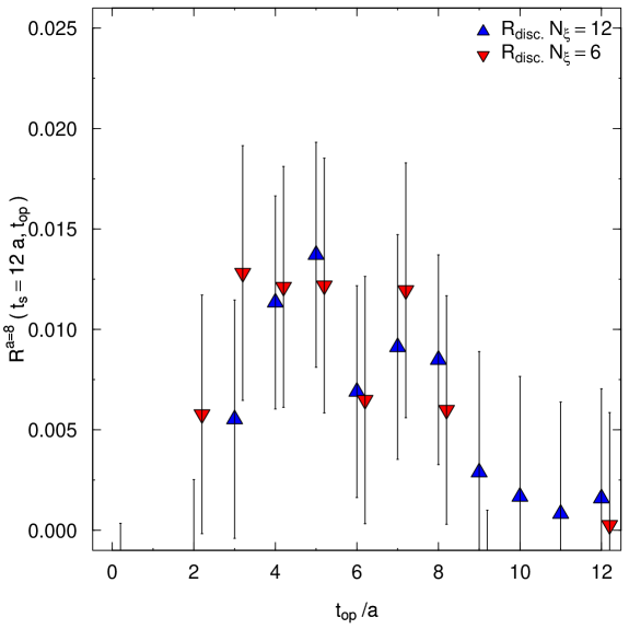
Figure 2: Plot of the contributions $R_{\rm{disc.}}$ versus $t_{\rm op}$ at $t_{s}=12a$ for $N_{\xi}=6$ (red down triangle) and $N_{\xi}=12$ (blue up triangle). The bare mass of the strange quark is fixed to $a\mu_{s}=0.018$ and we use $a\mu_{l}=0.0055$ and $\beta=1.95$

As a first step, we have investigated the magnitude of the stochastic noise introduced by the method described in section 2.3. To this end, we used a fixed number of gauge configurations for a gauge field ensemble at coupling $\beta=1.95$ and twisted mass parameter $a\mu_{l}=0.0055$. We show in Fig. 2, the ratio $R^{a=8}_{\rm{disc.}}$ for a fixed source-sink separation of $t_{s}\sim 1~{}\mathrm{fm}$ as a function of $t_{\rm op}$ for $N_{\xi}=6$ and $N_{\xi}=12$. As can be seen, the signal is compatible with zero within the errors when using $N_{\xi}=12$. Furthermore we observe that the error does not decrease much when the number of stochastic sources is doubled. This means presumably that the error is already dominated by the intrinsic noise of the gauge field fluctuations. We nevertheless decided to use $N_{\xi}=12$ throughout this benchmark study of the octet moment.

In principle, it would therefore be possible to reduce the error further by using more stochastic noise vectors. However, the contribution of the disconnected 3-point function is small compared to the value of the connected part as demonstrated in Fig. 3 where we show the connected contribution $R^{a=8}_{\rm{connected}}(t_{s}=12a,t_{\rm op})$, the disconnected contribution $R^{a=8}_{\rm{disconnected}}(t_{s}=12a,t_{\rm op})$ and the full correlator $R^{a=8}_{\rm{full}}(t_{s}=12a,t_{\rm op})$. In particular, the statistical errors on the connected part are about $~{}0.016$ ($\sim 2.5\%$) which is significantly larger than the size of the disconnected contributions. Despite this fact, which would make neglecting the dis-connected contributions tempting, we always include them in the following analysis. Note that the $R^{a=8}_{\rm{disconnected}}$ is proportional to the difference between the light and strange quark mass. Since we are using a mixed action setup, our results depends on an approximate tuning of the strange quark mass. In all the figures we use $a\mu_{s}(\beta=1.95)=0.018$ for $\beta=1.95$ and $a\mu_{s}(\beta=2.10)=0.015$ for $\beta=2.10$.f Those values can be compared to the values obtained for instance in Alexandrou:2014sha where the strange quark mass has been determined using the $\Omega^{-}$ mass and correspond to $a\mu_{s}(\beta=1.95)=0.0194$ and $a\mu_{s}(\beta=2.10)=0.0154$. However, by using data on the $\beta=1.95$ ensemble we have explicitly checked that changing the bare strange quark mass by more than $\sim 10\%$ does not lead to any significant change in the value of the disconnected contribution.

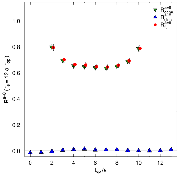
Figure 3: Plot of the contributions $R^{(8)}_{\rm{disconnected}}$ (blue triangle), $R^{(8)}_{\rm{connected}}$ (black triangles) and of their sum, $R^{(8)}_{\rm full}$ (red filled circles) as function of $t_{\rm op}$ at $t_{s}=12a$ for $a\mu_{l}=0.0055$ and $\beta=1.95$.

3.1 Excited states contamination

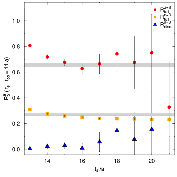
Figure 4: The ratio Eq. (12) as a function of the source-sink separation $t_{s}$ for a fixed source to operator time $t_{\rm op}=11a$ in the isovector (orange squares) and octet case (red dots). The gray bands indicate the results obtained from a fixed sink calculation for $t_{s}=12a$. The blue triangles show the disconnected contribution to $R^{a=8}(t_{s},t_{\rm op}=11a)$.

In order to investigate the contamination of excited states due to the second and third term in Eq. (12), we used the same procedure (”open-sink” method) as in Dinter:2011sg , namely we study the source-sink dependence for a fixed source to operator separation $t_{\rm op}\sim 0.9~{}\mathrm{fm}$ ( $t_{\rm op}=11a$). Details on the technical implementation of the ”open-sink” method can be found in Dinter:2011sg . To this end, a large statistics for the connected part ($\sim 23000$ measurements) has been used. We plot in Fig. 4 the resulting renormalized ratios $R^{a=3,8}(t_{s},t_{\rm op}=11a)$. The results in the isovector case are represented by orange squares and the results in the flavour octet case (including the disconnected piece) are depicted by red dots. We also represent using blue triangles the disconnected contribution to $R^{a=8}(t_{s},t_{\rm op}=11a)$. As can be seen, the noise for the dis-connected part dominates for large source-sink separation. Nevertheless, we can obtain a reasonable signal up to source-sink separation of about $16a$ ($\approx 1.3~{}\mathrm{fm}$). The gray bands indicate the values of $\langle x^{(a=3,8)}\rangle$ obtained using a fixed source-sink separation calculation with $t_{s}\sim 1~{}\mathrm{fm}$. Note that the fitting ranges have been determined choosing the fit with the longest plateau with a confidence level of least $90\%$. In the flavour octet case we observe that results obtained for $t_{s}/a>15$ and a fixed source-operator separation $t_{\rm op}=11a$ are compatible with the result obtained at a fixed source-sink separation of $t_{s}/a=12$. We mention that at the here used value of the pion mass of $m_{\rm{PS}}\approx 370~{}\mathrm{MeV}$, volume $(L=2.6~{}\mathrm{fm})$ and lattice spacing $(a\approx 0.082~{}\mathrm{fm})$ we found for the isovector channel a relative shift of about $10\%$ for a corresponding comparison at different source sink separationsDinter:2011sg .

We performed a similar study of the ratio of the octet to the singlet 3-point functions of Eq. (15),

$$R(t_{s},t_{\rm op})=C^{a=3}_{N,\rm 3pts}(t_{s},t_{\rm op})/C^{a=8}_{N,\rm 3pts}(t_{s},t_{\rm op}).$$ (26)

The ratio $R(t_{s},t_{op}=11a)$ is shown in Fig. 5 as a function of the source-sink separation $t_{s}$.The constant fit for this ratio obtained with a fixed source to operator time $t_{\rm op}=11a$ is depicted by a gray band. We used the same criterion as in Fig. 4 to determine the fitting range. In this case we do not observe any significant source-sink dependence of our results and thus there seem to be only a small excited states contamination, at least within the size of our errors. Note that the statistical errors stemming from the disconnected contribution are responsible for most of the total statistical error at large source-sink separation. In the next section we will use the difference between the central value at $t_{s}\sim 1.3\mathrm{fm}$ with the open think method and the central value obtained with the fixed source-sink method at $t_{s}\sim 1\mathrm{fm}$ as an estimate of the systematical error for $\langle x^{(a=3,8)}\rangle$ and $\frac{\langle x^{(3)}\rangle}{\langle x^{(8)}\rangle}$.

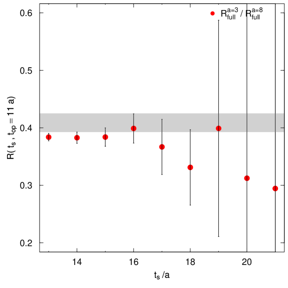
Figure 5: $\frac{R^{a=3}(t_{s},t_{\rm op}=11a)}{R^{a=8}(t_{s},t_{\rm op}=11a)}$ as a function of the source-sink separation $t_{s}$ for a fixed source to operator time $t_{\rm op}=11a$ (red dots). The gray band indicates the result obtained from a fixed sink calculation of $t_{s}=12a$.

3.2 Chiral behaviour

We plot our results for $\langle x^{(3,8)}\rangle_{\mu^{2}=4~{}\mathrm{GeV}^{2}}$ as a function of the pseudoscalar meson mass $m_{\rm{PS}}^{2}$ in Fig. 6. The results for $\langle x^{(3)}\rangle_{\mu^{2}=4~{}\mathrm{GeV}^{2}}$ (respectively $\langle x^{(8)}\rangle_{\mu^{2}=4~{}\mathrm{GeV}^{2}}$) are shown using red down triangles (resp. blue up triangle) for a lattice spacing of $0.082~{}\mathrm{fm}$ and by an orange square (resp. an orange dot) for a lattice spacing of $0.064~{}\mathrm{fm}$. Neglecting, in a first step, excited state contaminations and in order to investigate the chiral limit behaviour of our data, all the results have been obtained using a fixed source-sink separation of approximately $1~{}\mathrm{fm}$. Of course, in our final result we will add the shift from the excited states contamination as a systematic error. As can be seen in Fig. 6 the results obtained at two different lattice spacings are compatible, and ${\mathcal{O}}(a^{2})$ effects can be neglected.

The phenomenological estimates Sergey of Eq. (3) are represented by two black stars. As can be seen in the graph, for both, $\langle x^{(3)}\rangle$ and $\langle x^{(8)}\rangle$ and for unphysically large values of the pion mass the lattice data lay consistently above the phenomenological values, a phenomenon that is well know from previous investigations of $\langle x^{(3)}\rangle$, see e.g. Constantinou:2014tga , and is here demonstrated for the first time for $\langle x^{(8)}\rangle$.

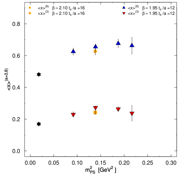
Figure 6: $\langle x^{(3,8)}\rangle_{\mu^{2}=4~{}\mathrm{GeV}^{2}}$ as a function of the pseudoscalar meson mass $m_{\rm{PS}}^{2}$. The phenomenological estimates are represented by two black stars.

As explained before, systematic errors stemming from discretization effects and from the matching mass dependence can be neglected. With the present data set we cannot estimate safely the volume dependence of $\langle x^{(3,8)}\rangle$, however knowing that they are negligible in the isovector case in our $N_{f}=2$ calculation Alexandrou:2011nr we assume them to be small and neglect them, too. Our dominating source of systematic error for the individual matrix elements is then due to the excited states contamination. In addition, as the chiral extrapolation is not performed here, it remains as a presently unquantifiable systematic error.

In fig. 7 we show the ratio $\frac{\langle x^{(3)}\rangle}{\langle x^{(8)}\rangle}$ as a function of the pion mass together with the phenomenological value. Here the situation is somewhat different in that the lattice data agree with the phenomenological analysis even at the here used unphysically large pion masses. This suggests that some of the systematic uncertainties cancel in the ratio. As discussed in section 3.1, the systematic error stemming from the excited states contamination is negligible for the ratio $\frac{\langle x^{(3)}\rangle}{\langle x^{(8)}\rangle}$. Therefore, we conclude for the individual moments that either the non-perturbative renormalization or the chiral extrapolation is the most probable systematic effect leading to the observed discrepancies in $\langle x^{(3,8)}\rangle$. It would therefore be highly desirable to perform simulations directly at the physical point to eliminate the uncertainty from the chiral extrapolation. Work in this direction is in progress Abdel-Rehim:2013yaa ; Abdel-Rehim:2014nka .

Since the lattice data are flat as function of the pion mass, we perform a simple constant extrapolation to the physical pion mass. As a systematic error, we take the difference between the data points at the smallest and the largest pion mass. We find then for $\langle x^{(a=3)}\rangle_{\mu^{2}=4~{}\mathrm{GeV}^{2}}/\langle x^{(a=8)}\rangle_{\mu^{2}=4~{}\mathrm{GeV}^{2}}$

$$\frac{\langle x^{(3)}\rangle}{\langle x^{(8)}\rangle}=0.39(1)(4)\;$$ (27)

where the first error is statistical and the second one is our estimate of the systematic error. When comparing to phenomenological extractions Sergey we find that the ratio $\frac{\langle x^{(3)}\rangle}{\langle x^{(8)}}$ is, within errors, compatible with phenomenological extractions at least for the here used simple extrapolation to the physical point.

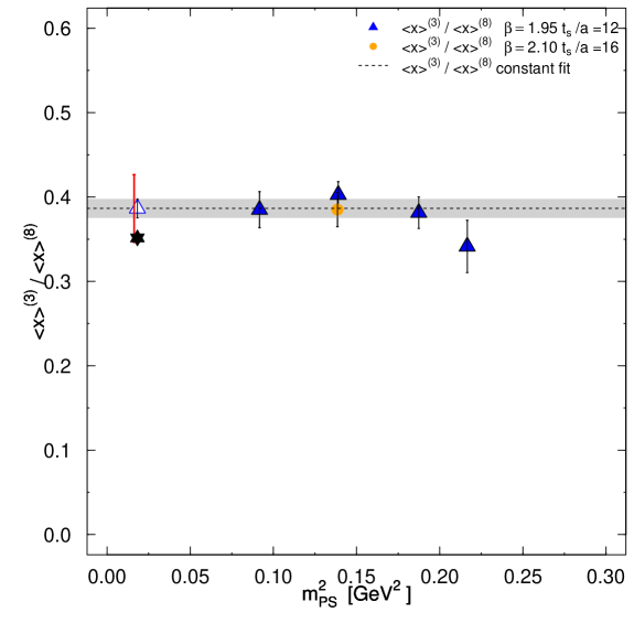
Figure 7: $\langle x^{(a=3)}\rangle_{\mu^{2}=4~{}\mathrm{GeV}^{2}}/\langle x^{(a=8)}\rangle_{\mu^{2}=4~{}\mathrm{GeV}^{2}}$ as a function of the pseudoscalar meson mass $m_{\rm{PS}}^{2}$ for two values of the lattice spacing. The result of a constant extrapolation is represented by an empty triangle. The systematic error on the extrapolated value is represented by a red error bar slightly shifted for readability. The phenomenological estimate from is represented by a black star.

4 Conclusion

In this work we have performed a benchmark computation of the flavour octet combination of the first moment of parton distribution functions of the nucleon using $N_{f}=2+1+1$ twisted mass fermions tuned to maximal twist. This quantity can provide a first hint of the contribution of the strange quark to the quark momentum in the nucleon. We have utilized the fact that $\langle x\rangle^{(8)}_{\mu^{2}}$ shares the same renormalization property as the standard iso-vector moment $\langle x\rangle^{(3)}_{\mu^{2}}$. Using our result for the non-perturbative renormalization constant obtained in Alexandrou:2013joa we can thus provide an ${\mathcal{O}}(a^{2})$ improved estimate of $\langle x\rangle^{(8)}_{\mu^{2}}$. The calculation takes into account the notably noisy dis-connected contribution, which are shown to have a negligible contribution in our setup.

In our investigation of $\langle x\rangle^{(8)}_{\mu^{2}}$ we found, similar to the case of $\langle x\rangle^{(3)}_{\mu^{2}}$ Dinter:2011sg , that the excited states contamination can be substantial and has to be taken into account as a systematic error. We also found that, similar to the case of $\langle x\rangle^{(3)}_{\mu^{2}}$, the lattice data for $\langle x\rangle^{(8)}_{\mu^{2}}$ are systematically higher than the phenomenological value, see fig. 6 for pion masses larger than the physical one.

However, when the ratio $\langle x^{(a=3)}\rangle_{\mu^{2}=4~{}\mathrm{GeV}^{2}}/\langle x^{(a=8)}\rangle_{\mu^{2}=4~{}\mathrm{GeV}^{2}}$ is considered, the lattice data show an overall agreement with the corresponding phenomenological ratio, indicating that in the ratio systematic errors cancel. Since in the ratio the excited states contamination is small, the here observed agreement cannot be due to this systematic uncertainty. One reason why the ratio agrees with the phenomenological value can be that the renormalization constants cancel. Another possibility is that both, $\langle x\rangle^{(8)}_{\mu^{2}}$ and $\langle x\rangle^{(3)}_{\mu^{2}}$ have a very similar chiral limit behaviour such that the effects from the chiral extrapolation cancel. It would be highly desirable to have therefore lattice results directly at the physical point for both quantities. Since the lattice data are rather flat, we performed a simple constant extrapolation to the physical point for the ratio $\langle x^{(a=3)}\rangle_{\mu^{2}=4~{}\mathrm{GeV}^{2}}/\langle x^{(a=8)}\rangle_{\mu^{2}=4~{}\mathrm{GeV}^{2}}$ and find

$$\frac{\langle x^{(3)}\rangle}{\langle x^{(8)}\rangle}=0.39(1)(4)$$ (28)

This value is in agreement with the phenomenological extraction of this quantity from deep inelastic scattering data Sergey .

References

- (1) ETM Collaboration Collaboration, S. Dinter et. al., Sigma terms and strangeness content of the nucleon with twisted mass fermions, JHEP 1208 (2012) 037, [arXiv:1202.1480].
- (2) C. Alexandrou, M. Constantinou, S. Dinter, V. Drach, K. Jansen, et. al., Nucleon form factors and moments of generalized parton distributions using twisted mass fermions, Phys.Rev. D88 (2013) 014509, [arXiv:1303.5979].
- (3) C. Alexandrou, J. Carbonell, M. Constantinou, P. Harraud, P. Guichon, et. al., Moments of nucleon generalized parton distributions from lattice QCD, Phys.Rev. D83 (2011) 114513, [arXiv:1104.1600].
- (4) C. Alexandrou, M. Brinet, J. Carbonell, M. Constantinou, P. Harraud, et. al., Nucleon electromagnetic form factors in twisted mass lattice QCD, Phys.Rev. D83 (2011) 094502, [arXiv:1102.2208].
- (5) ETM Collaboration Collaboration, C. Alexandrou et. al., Axial Nucleon form factors from lattice QCD, Phys.Rev. D83 (2011) 045010, [arXiv:1012.0857].
- (6) G. Bali, S. Collins, B. Gläßle, M. Göckeler, J. Najjar, et. al., Nucleon generalized form factors and sigma term from lattice QCD near the physical quark mass, arXiv:1312.0828.
- (7) G. S. Bali, S. Collins, M. Deka, B. Glassle, M. Gockeler, et. al., from lattice QCD at nearly physical quark masses, Phys.Rev. D86 (2012) 054504, [arXiv:1207.1110].
- (8) J. Green, M. Engelhardt, S. Krieg, J. Negele, A. Pochinsky, et. al., Nucleon Structure from Lattice QCD Using a Nearly Physical Pion Mass, arXiv:1209.1687.
- (9) LHPC Collaborations Collaboration, P. Hagler et. al., Nucleon Generalized Parton Distributions from Full Lattice QCD, Phys.Rev. D77 (2008) 094502, [arXiv:0705.4295].
- (10) C. Alexandrou, M. Constantinou, V. Drach, K. Hatziyiannakou, K. Jansen, et. al., Nucleon Structure using lattice QCD, Nuovo Cim. C036 (2013), no. 05 111–120, [arXiv:1303.6818].
- (11) M. Constantinou, Hadron Structure, PoS LATTICE2014 (2014) 001, [arXiv:1411.0078].
- (12) S. Alekhin, J. Bluemlein, and S. Moch, The ABM parton distributions tuned to LHC data, Phys.Rev. D89 (2014) 054028, [arXiv:1310.3059].
- (13) S. Alekhin, Private communication, .
- (14) C. Alexandrou, M. Constantinou, V. Drach, K. Hadjiyiannakou, K. Jansen, et. al., Evaluation of disconnected quark loops for hadron structure using GPUs, Comput.Phys.Commun. 185 (2014) 1370–1382, [arXiv:1309.2256].
- (15) C. Alexandrou, M. Constantinou, S. Dinter, V. Drach, K. Hadjiyiannakou, et. al., Strangeness of the nucleon from Lattice Quantum Chromodynamics, arXiv:1309.7768.
- (16) A. Abdel-Rehim, C. Alexandrou, M. Constantinou, V. Drach, K. Hadjiyiannakou, et. al., Disconnected quark loop contributions to nucleon observables in lattice QCD, Phys.Rev. D89 (2014), no. 3 034501, [arXiv:1310.6339].
- (17) Y. Iwasaki, Renormalization Group Analysis of Lattice Theories and Improved Lattice Action: Two-Dimensional Nonlinear O(N) Sigma Model, Nucl. Phys. B258 (1985) 141–156.
- (18) Alpha Collaboration, R. Frezzotti, P. A. Grassi, S. Sint, and P. Weisz, Lattice QCD with a chirally twisted mass term, JHEP 0108 (2001) 058, [hep-lat/0101001].
- (19) R. Frezzotti and G. C. Rossi, Chirally improving Wilson fermions. I: O(a) improvement, JHEP 08 (2004) 007, [hep-lat/0306014].
- (20) R. Frezzotti and G. C. Rossi, Twisted-mass lattice qcd with mass non-degenerate quarks, Nucl. Phys. Proc. Suppl. 128 (2004) 193–202, [hep-lat/0311008].
- (21) R. Frezzotti and G. C. Rossi, Chirally improving wilson fermions. ii: Four-quark operators, JHEP 10 (2004) 070, [hep-lat/0407002].
- (22) R. Baron et. al., Light hadrons from lattice QCD with light (u,d), strange and charm dynamical quarks, JHEP 06 (2010) 111, [arXiv:1004.5284].
- (23) European Twisted Mass Collaboration, R. Baron et. al., Computing K and D meson masses with twisted mass lattice QCD, arXiv:1005.2042.
- (24) European Twisted Mass Collaboration, C. Alexandrou et. al., Light baryon masses with dynamical twisted mass fermions, Phys. Rev. D78 (2008) 014509, [arXiv:0803.3190].
- (25) ETM Collaboration Collaboration, C. Michael and C. Urbach, Neutral mesons and disconnected diagrams in Twisted Mass QCD, PoS LAT2007 (2007) 122, [arXiv:0709.4564].
- (26) ETM Collaboration, P. Boucaud et. al., Dynamical Twisted Mass Fermions with Light Quarks: Simulation and Analysis Details, Comput. Phys. Commun. 179 (2008) 695–715, [arXiv:0803.0224].
- (27) C. Alexandrou, M. Constantinou, T. Korzec, H. Panagopoulos, and F. Stylianou, Renormalization constants for 2-twist operators in twisted mass QCD, Phys.Rev. D83 (2011) 014503, [arXiv:1006.1920].
- (28) ETM Collaboration Collaboration, B. Blossier et. al., Renormalization of quark propagator, vertex functions and twist-2 operators from twisted-mass lattice QCD at =4, arXiv:1411.1109.
- (29) B. Blossier, M. Brinet, P. Guichon, V. Morénas, O. Pène, et. al., Renormalization constants for twisted mass QCD, arXiv:1411.0053.
- (30) C. Alexandrou, V. Drach, K. Jansen, C. Kallidonis, and G. Koutsou, Baryon spectrum with twisted mass fermions, arXiv:1406.4310.
- (31) S. Dinter, C. Alexandrou, M. Constantinou, V. Drach, K. Jansen, et. al., Precision Study of Excited State Effects in Nucleon Matrix Elements, Phys.Lett. B704 (2011) 89–93, [arXiv:1108.1076].
- (32) A. Abdel-Rehim, P. Boucaud, N. Carrasco, A. Deuzeman, P. Dimopoulos, et. al., A first look at maximally twisted mass lattice QCD calculations at the physical point, PoS LATTICE2013 (2014) 264, [arXiv:1311.4522].
- (33) A. Abdel-Rehim, C. Alexandrou, P. Dimopoulos, R. Frezzotti, K. Jansen, et. al., Progress in Simulations with Twisted Mass Fermions at the Physical Point, PoS LATTICE2014 (2014) 119, [arXiv:1411.6842].