Energy in density gradient

Abstract

Inhomogeneous plasmas and fluids contain energy stored in inhomogeneity and they naturally tend to relax into lower energy states by developing instabilities or by diffusion. But the actual amount of energy in such inhomogeneities has remained unknown. In the present work the amount of energy stored in a density gradient is calculated for several specific density profiles in a cylindric configuration. This is of practical importance for drift wave instability in various plasmas, and in particular in its application in models dealing with the heating of solar corona because the instability is accompanied with stochastic heating, so the energy contained in inhomogeneity is effectively transformed into heat. It is shown that even for a rather moderate increase of the density at the axis in magnetic structures in the corona by a factor 1.5 or 3, the amount of excess energy per unit volume stored in such a density gradient becomes several orders of magnitude greater than the amount of total energy losses per unit volume (per second) in quiet regions in the corona. Consequently, within the life-time of a magnetic structure such energy losses can easily be compensated by the stochastic drift wave heating.

I Introduction

From standard theory it is known that an isothermal system with the volume $V$, consisting of several species $j$ and with the total number of particles for each species $N_{j}$, contains a total amount of internal energy in the given volume $U_{int}\equiv U_{t}=(3\kappa T/2)\sum_{j}N_{j}$, which is just the thermal energy of the system.

This internal energy may be modified in various ways. For example, if the species are charged and they include electrons and ions, the chaotic thermal motion is affected by the Coulomb interaction. The internal energy in this case contains such a contribution and it is reduced:

$$U_{int}=U_{t}\left[1-\frac{1}{12\pi}\left(\frac{d}{r_{d}}\right)^{3}\right].$$ (1)

Here, $d$ is the mean distance between the charged particles and $r_{d}$ is the plasma Debye radius. Such a modification of the internal energy implies also modifications of all other thermodynamic functions; i.e., the free energy, pressure, and entropy are all reduced, and the heat capacity increased. One example of this kind, dealing with dusty plasmas, may be found in Pandey & Vranjes (2005). In most of electron-ion plasmas the Coulomb correction is small (implying a relatively large amount of particles within the Debye sphere), and such plasmas are then called ideal, or weakly non-ideal ones.

The total internal energy (and thus all other thermodynamic functions as well) may change also in the presence of some external forces. Without such forces a gas or plasma system will tend to relax into an energetically most favorable state with minimum energy, and this usually means it will become isothermal and homogeneous. However, these external forces may cause gradients of various quantities, like density, temperature etc., and the internal energy (1) and other thermodynamic functions will change. Classic studies dealing with the free energy and thermodynamics of an inhomogeneous environment may be found in works Cahn & Hilliard (1958); Hart (1959); Rice & Chang (1974); Silver (1978); McCoy & Davis (1979); Warner (1980), and Lowett & Baus (1992). These works mainly contain a general theory while for practical purposes some explicit results for the free energy are needed, and such an analysis will be performed in the present work.

The presence of such gradients implies an excess of energy, and the system will tend to get rid of it through diffusion of particles until the minimum energy state is achieved, or much more efficiently by developing various instabilities, including drift instabilities as one example of general interest for plasmas. Drift instabilities in an inhomogeneous environment represent an efficient way of relaxation towards a lower energy state, and they are present in almost every realistic plasma configuration. In the laboratory plasmas they represent a major issue for confinement, though the actual amount of energy stored in the plasma inhomogeneity has not been calculated so far. For various purposes it may be very useful and instructive to know in advance the total amount of this extra energy. For example, this may help in modeling stochastic heating based on such drift instabilities, in particular in the solar corona environment, suggested recently in a series of our works.(Vranjes & Poedts, 2009a, b, c, d, 2010a, 2010b)

In the present work the excess energy stored in the density gradient is calculated for some relatively simple density profiles. The obtained results should be applicable to various plasmas both in the laboratory and in space, and to fluids in general.

II Energy in density gradient

We shall assume a cylindric volume $V=\pi R^{2}L_{z}$ inhomogeneous due to some external forces, where $R$ is the radius and $L_{z}$ is the axial length. For example, in the presence of a magnetic field the radial density gradient, or pressure gradient in general, may be counteracted by the magnetic pressure. This in principle implies the presence of the radial inhomogeneity of the magnetic field as well, which can be small in case of a small plasma-beta, (Vranjes, 2011, 2011) yet in any case it is supposed to balance the assumed pressure (density) gradient. But quite generally, the quasi-static equilibrium may be described through the balance of forces

$$0=-\nabla p+\sum_{l}\vec{F}_{l}.$$ (2)

So we may proceed by taking such a density gradient as a fact, knowing that it must imply additional forces acting on the plasma, and this means that it is not in the minimum energy state. In other words, once such external forces are removed, or due to collisions and diffusion, the plasma will naturally relax into the lowest possible energy state, occupying thus the whole volume $V$ and having some constant number density $n_{h}$ and a constant temperature.

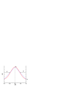
Figure 1: Sketch of the two density profiles, linear and Gaussian, in a cylindric volume $V=\pi R^{2}L_{z}$, in balance with some radially acting force $\vec{F}$.

Our inhomogeneous system thus has some radially dependent density $n(r)$, and we shall calculate its internal energy (which includes thermal and potential energy) taking several possible cases for the density shape.

Figure 2: Coronal magnetic structures, picture taken by the Transition Region and Coronal Explorer (TRACE).(TRACE, 2014)

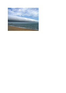
Figure 3: A roll cloud pictured in Uruguay. (Wikipedia, 2014)

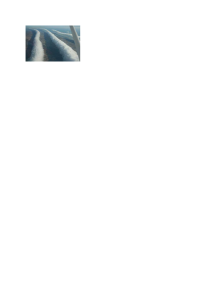
Figure 4: Multiple roll clouds pictured in Australia. (Wikipedia, 2014)

The theory presented here may be applicable to coronal magnetic structures(TRACE, 2014) [see Fig. 2], and to some atmospheric phenomena like roll clouds and bores. Roll clouds are tube-shaped, many kilometers long structures rolled up about a horizontal axis, single (Wikipedia, 2014) or multiple Wikipedia (2014) [see Figs. 3, 4], like so called Morning Glory cloud frequently observed in Australia(Smith, 1988) that can be between hundred and thousand kilometers long and only about one kilometer in diameter,(Rottman & Grimshaw, 2004; Goler & Reeder, 2004) and also clouds observed in South America and elsewhere.(Wikipedia, 2014; Hartung & Sitkowski, 2010) A clear pressure jump of up to 200 Pa in such rolling solitons has been measured, (Goler & Reeder, 2004) implying the excess of energy in them as compared with the surrounding fluid. Yet another atmospheric example of similar kind are tornados.

In derivations further in the text, the potential and internal energies are per species, so the theory is valid for ordinary fluids, and in electron-ion plasmas (or multi-component in general with a number of species $\mu$) all expressions should be multiplied by a factor 2 (or by factor $\mu$).

II.1 Linear density profile with porous boundaries

We shall assume a nearly ideal plasma with a negligible Coulomb interaction energy and having a linear number density profile

$$n(r)=n_{0}-ar.$$ (3)

The number density has the value $n_{\scriptscriptstyle R}$ at the edge of the cylinder with the radius $R$, and it increases towards the axis to a maximum value $n_{0}$, see Fig. 1, the dashed line. This means that $a=(n_{0}-n_{\scriptscriptstyle R})/R$. It will be shown later that the expected results for the internal energy should not be much different from some more realistic cases, like the Gaussian profile presented in the same figure. Note that in some cases, like in some magnetic configuration in the solar plasma, the profile may be just inverted, with a decreasing density towards the axis, implying forces acting in the opposite direction. However, there will again be a resulting potential energy stored in the inhomogeneity.

If the forces are removed, or due to collisions, in time the system will relax to the minimum energy homogeneous state with some constant density $n_{h}$. In space or in solar plasma we may assume that this extra density in the gradient from Fig. 1 will be absorbed by the infinite reservoir of the plasma around with the assumed density $n_{\scriptscriptstyle R}$. So the potential energy will be calculated with respect to $n_{\scriptscriptstyle R}$, and this we shall call the model of porous or absorbing boundaries. In such environments this is rather justified. However, in bounded plasmas and fluids in the laboratory, the relaxed density will clearly have some value $n_{h}>n_{\scriptscriptstyle R}$. This issue shall be addressed later completely exactly in Sec. III.

The total number of particles in the volume $V$ is $N=\int n(r)dV$, where $dV=rdrd\theta dz$ and integration is over the angle $\theta\in(0,2\pi)$, over $z\in(0,L_{z})$, and $r\in(0,R)$. Eventual variation of density in $z$ and $\theta$ directions is neglected. The result is:

$$N=V\frac{n_{0}+2n_{\scriptscriptstyle R}}{3}.$$ (4)

The thermal energy for the case of inhomogeneous density is $U_{t}=\int(3\kappa T/2)n(r)dV$. For the density (3) and with the boundary conditions $n(0)=n_{0}$, $n(R)=n_{\scriptscriptstyle R}$ this yields

$$U_{t}=V\kappa T\left(\frac{n_{0}}{2}+n_{\scriptscriptstyle R}\right).$$ (5)

In view of Eq. (2), the internal energy in the present case must be the sum of the thermal energy $U_{t}$ and some potential energy which system has achieved due to the work of the external forces $\sum_{l}\vec{F}_{l}$. In principle, presently we are not interested in separate forces $\vec{F}_{l}$, but we shall use the fact that their total sum exactly matches the pressure force. So in order to calculate the potential energy it may be convenient to use the pressure force instead of $\sum_{l}\vec{F}_{l}$, and express the potential energy through the temperature and density only.

The potential energy $E_{1}(r)$ of a unit volume at some position $r$, obtained by the act of forces acting on it, is the integral over the distance and it can be written as

$$E_{1}(r)=\int^{r}\sum_{l}\vec{F}_{l}(r^{\prime})d\vec{r^{\prime}}=\int^{r}\!\!\nabla pd\vec{r^{\prime}}=\kappa Tn_{1}(r).$$ (6)

The number density $n(r)$ has the lowest value $n_{\scriptscriptstyle R}$ at the boundary, and in case of some large configurations in the atmosphere or in space, like solar magnetic structures this value will be assumed the same outside for $r>R$ (porous or absorbing boundary). Inside the structure, clearly the excess density above $n_{\scriptscriptstyle R}$ will contain additional potential energy due to action of forces, see Fig. 1. Thus the density $n_{1}$ in Eq. (6) satisfies the following boundary conditions: $n_{1}(0)=n_{0}-n_{\scriptscriptstyle R}$, and $n_{1}(R)=0$. This yields $n_{1}(r)=(n_{0}-n_{\scriptscriptstyle R})(1-r/R)$.

The total potential energy in the volume $V$ is thus the integral of $E_{1}(r)$ over the whole volume and it reads:

$$E_{p}=V\kappa T\frac{n_{0}-n_{\scriptscriptstyle R}}{3}.$$ (7)

The total internal energy is the sum of the two, $U_{int}=U_{t}+E_{p}$, and the Gibbs-Helmholtz thermodynamic free energy $F$ can easily be obtained using the well known relation

$$U_{int}=-T^{2}\frac{\partial}{\partial T}\left(\frac{F}{T}\right)_{V}.$$

The specific heat and entropy are given by $C_{v}=\partial U_{int}/\partial T|_{\scriptscriptstyle V}$, $S=-\partial F/\partial T|_{\scriptscriptstyle V}$. However, for the drift instabilities only the potential part of the internal energy may play the role, and Eq. (7) shows that it is present as long as $n_{\scriptscriptstyle R}\neq n_{0}$.

II.2 Gaussian and arbitrary flat-top density profile

For a Gaussian density profile (the full line in Fig. 1) $n(r)=c_{1}\exp(-ar^{2})+c_{2}$, where $c_{1},c_{2}$ are chosen to satisfy the boundary conditions $n(0)=n_{0}$, $n(R)=n_{\scriptscriptstyle R}$, we have

$$n(r)=n_{0}-b\left[1-\exp(-ar^{2})\right],\quad b=\frac{n_{0}-n_{\scriptscriptstyle R}}{1-\exp(-aR^{2})}.$$ (8)

This is used to calculate the thermal energy. The result is

$$U_{t}=\frac{3}{2}V\kappa T[\alpha(n_{0}-n_{\scriptscriptstyle R})+n_{\scriptscriptstyle R}],$$ (9)

$$\alpha=1+\frac{1}{aR^{2}}-\frac{1}{1-\exp(-aR^{2})}.$$

For the potential energy the boundary conditions are as before $n_{1}(0)=n_{0}-n_{\scriptscriptstyle R}$, $n_{1}(R)=0$, i.e., the density (8) is reduced by $n_{\scriptscriptstyle R}$. The mean potential energy per unit volume now becomes

$$\frac{E_{p}}{V}=\kappa T\alpha(n_{0}-n_{\scriptscriptstyle R}).$$ (10)

Comparing this with Eq. (7) it is seen that the potential energy in the present case may be greater than the value obtained for the linear density profile providing that $\alpha>1/3$. Note that $\alpha\rightarrow 0.5$ when $aR^{2}\rightarrow 0$, and $\alpha\rightarrow 0$ when $aR^{2}\rightarrow\infty$, and $\alpha\approx 0.42$ when $aR^{2}\approx 1$. So the differences between the two profiles are not drastic in any case. The total internal energy is consequently

$$U_{int}=U_{t}+E_{p}=\frac{V\kappa T}{2}\left[5\alpha(n_{0}-n_{\scriptscriptstyle R})+3n_{\scriptscriptstyle R}\right].$$

Instead of the Gaussian density we may have an arbitrary flat-top profile which can be found in numerous plasmas $n(r)=c_{1}\exp(-ar^{k})+c_{2}$, where again $c_{1},c_{2}$ are chosen to satisfy $n(0)=n_{0}$, $n(R)=n_{\scriptscriptstyle R}$. For $k=2$ this yields the Gaussian case discussed above, and in the limit $k\rightarrow\infty$ it gives a step-profile. Repeating the calculation presented above we obtain the potential energy density (10) where now

$$\alpha=1-\frac{1}{1-\exp(-aR^{k})}$$

$$-\frac{2}{R^{2}}\frac{1}{1-\exp(-aR^{k})}\frac{a^{-2/k}}{k}\left(\Gamma[2/k,ar^{k}]\right)^{R}_{0},$$ (11)

and $\Gamma[b,x]$ is the incomplete Euler gamma function.

In fact, the analysis can easily be generalized to any density profile in the cylindric system, bearing in mind the procedure described above. The result for the potential energy is

$$E_{p}=V\frac{2\kappa T}{R^{2}}\int_{0}^{R}\left[n(r)-n_{\scriptscriptstyle R}\right]rdr,$$ (12)

and the thermal energy is $U_{t}=3\pi\kappa TL_{z}\int_{0}^{R}n(r)rdr=(V3\kappa T/R^{2})\int_{0}^{R}n(r)rdr$.

II.3 Application to heating in the solar corona

The solar corona is hot and it continuously looses its energy. Without an efficient generator of energy, the amount expressed through Eq. (1) would be lost in less than a day and the corona would become completely cool. However, it remains hot and with the temperature exceeding a million degrees.

The presence of the density gradient implies drift instabilities and those may lead to stochastic heating if certain conditions are satisfied. (Hatakeyama et al., 1980; McChesney et al., 1987, 1991; Sanders et al., 1998) We shall make some estimate and application of the present results to the drift wave heating paradigm in the solar atmosphere, which we put forward recently.(Vranjes & Poedts, 2009a, b, c, d, 2010a, 2010b)

For the quiet regions in the solar corona, presently accepted required heating rate, (Narain & Ulmschenider, 1990) with the temperature $T=1.8\cdot 10^{6}$ K, is in the range $\Gamma_{0}\equiv E_{0}/s=2\cdot 10^{-7}$ J/(m³s) to $\Gamma_{0}=4\cdot 10^{-6}$ J/(m³s) for the two number densities $n_{q}=0.2\cdot 10^{15}$ m^-3 and $n_{q}=10^{15}$ m^-3, respectively. Note that for such parameters the corrections due to Coulomb interaction in Eq. (1) are completely negligible. Such a heating rate can easily be satisfied in the solar magnetic structures following the models based on the drift wave stochastic heating.(Vranjes & Poedts, 2009a, b, c, d, 2010a, 2010b) In these studies various heating rate values are obtained, dependent on the plasma parameters. As example, in magnetic structures with the characteristic inhomogeneity scale-length $L_{n}$ of around several hundred kilometers, the wave frequency is of the order of 0.1 Hz and the energy release rate $\Gamma$ due to the stochastic heating is around the value $\Gamma_{0}$ given above, see more in Vranjes & Poedts (2009a).

We may now take some specific density profile and calculate the potential energy density $E_{1}=E_{p}/V$ for the heating rate $\Gamma\simeq\Gamma_{0}$ in order to see at least roughly for how long such a density profile might sustain the plasma at the given temperature, i.e., for how long it may compensate for the energy losses. The result is presented in Table 1 and Table 2 for the temperature and two starting densities for quiet regions $n_{\scriptscriptstyle R}=n_{q}$ given above, and allowing for several possible density values $n_{0}$ in the center of the loop. From Table 1 it is seen that even in the case when the boundary value $n_{\scriptscriptstyle R}$ increases only by a factor 1.5 at the axis, the mean potential energy density becomes $E_{1}=E_{p}/V=8.3\cdot 10^{-4}$ J/m³, which is several orders of magnitude greater than the energy lost per unit volume in one second. This is even more so for the values in Table 2. But in reality, the density gradient changes (i.e., the density profile flattens) in time and so does the realistic energy release rate; observations show that the mean life time of the loops is in the range of half an hour to a few hours. So to make some estimate we may set the loop life-time equal one hour, and to have a realistic margin and to be sure about a sustainable heating it would be necessary to have the ratio $E_{1}/E_{0}$ considerably greater than 3600. The numbers given in Tables 1, 2 show that this is indeed the case for almost all values of $n_{0}$. Observe also that the potential energy becomes a considerable part of the total internal energy already for $n_{\scriptscriptstyle R}/n_{0}>3$. As stressed before, the numbers presented here are per species.

A similar analysis can be performed for the coronal holes where $\Gamma_{0}=8\cdot 10^{-6}$ J/(m³s), showing that the amount of energy in the density gradient is more than enough for a sustainable heating.

Table 1: Parameters for quiet regions following Narain & Ulmschenider (1990) with $n_{\scriptscriptstyle R}=0.2\cdot 10^{15}$ m^-3 and for linear density profile given by Eq. (3), with several values $n_{0}$ at the center.

$n_{0}/n_{\scriptscriptstyle R}$	1.5	3	5	10
$E_{1}$ [J/m3]	0.0008	0.0033	0.0066	0.015
$U_{th}/V$ [J/m3]	0.0087	0.012	0.017	0.03
$E_{p}/U_{th}$	0.095	0.27	0.38	0.5
$E_{1}/E_{0}$	4142	16568	33137	74558

Table 2: Parameters for quiet regions following Narain & Ulmschenider (1990) with $n_{\scriptscriptstyle R}=10^{15}$ m^-3 and for linear density profile (3).

$n_{0}/n_{\scriptscriptstyle R}$	1.5	3	5	10
$E_{1}$ [J/m3]	0.0041	0.0165	0.033	0.074
$U_{th}/V$ [J/m3]	0.043	0.062	0.087	0.15
$E_{p}/U_{th}$	0.095	0.27	0.38	0.5
$E_{1}/E_{0}$	20710	82842	165684	372789

In active regions, following Narain & Ulmschenider (1990) the temperature and the number density vary from $T=10^{4}$ K, $n_{a}=0.5\cdot 10^{15}$ m^-3 to $T=2.5\cdot 10^{6}$ K, $n_{a}=5\cdot 10^{15}$ m${}^{-3}=n_{\scriptscriptstyle R}$, and the energy losses are in the range $\Gamma_{0}=7\cdot 10^{-5}$ J/(m³s) to $\Gamma_{0}=3\cdot 10^{-4}$ J/(m³s). For the first set of data a sustainable heating $\Gamma\simeq\Gamma_{0}$ appears possible for a few second only, provided that $n_{0}=10n_{\scriptscriptstyle R}$. However, for the second set $T=2.5\cdot 10^{6}$ K, $n_{a}=5\cdot 10^{15}$ m^-3 the situation is a bit different, and the result is presented in Table 3. These data indicate that a rather strong density gradient is needed to sustain the energy losses within the life-time of a magnetic structure in active regions.

Table 3: Parameters for active regions following Narain & Ulmschenider (1990) with $T=2.5\cdot 10^{6}$ K, $n_{a}=5\cdot 10^{15}$ m^-3, for linear density profile (3), and with several values $n_{0}$ at the center.

$n_{0}/n_{\scriptscriptstyle R}$	1.5	3	5	10	15
$E_{1}=E_{p}/V$ [J/m3]	0.03	0.115	0.23	0.52	0.18
$U_{th}/V$ [J/m3]	0.3	0.43	0.6	1.04	1.47
$E_{p}/U_{th}$	0.095	0.27	0.38	0.5	0.55
$E_{1}/E_{0}$	96	383	767	1726	2685

The analysis presented above can be repeated for the Gaussian density profile (8). Without going into details, we may take the case $aR^{2}\approx 1$, and in view of Eqs. (7, 10) it may be shown that the above given values for the heating time should be multiplied by a factor 1.26. So the heating in this case in quiet regions and coronal holes is even more certain and this holds for all cases with $aR^{2}<1$.

The calculated potential energy stored in the density gradient and the consequent stochastic heating by the drift wave are thus more than enough to compensate for losses in quiet Sun regions and in coronal holes, and the predicted sustainable stochastic heating(Vranjes & Poedts, 2009a, b, c, d, 2010a, 2010b) by the drift wave looks like a rather realistic scenario. In active regions it may sustain heating only provided relatively strong density gradients as Table 3 suggests, so most likely some additional and more energetic processes are in action in such regions.

III Non-absorbing boundaries

In the laboratory environment the initial density profile with the number density $n_{\scriptscriptstyle R}$ at the edge of the cylinder will normally relax to a homogeneous minimum available energy state with the density line $n=n_{h}$, see Fig. 5. We shall use this simple linear density for the present analysis although obviously it can easily be replaced with the Gaussian one as shown in Sec. II. Quantitatively, the results will be similar. Clearly there must be $n_{\scriptscriptstyle R}<n_{h}<n_{0}$ as depicted in Fig. 5. The same situation may sometimes happen also in coronal magnetic structures with exceptionally strong boundary magnetic field when diffusion across the boundary itself is much weaker as compared with the diffusion inside the structure and when there are drift instabilities taking place inside the structure. In this case the density $n_{h}$ would correspond to the density of the bulk plasma around the structure. A more realistic situation in coronal structures is presented in Fig. 6 where we have the external density $n_{h}$, and the given density inside the structure, which is a more physical variant of the rough profile from Fig. 5.

Note that the assumed actual linear density profile in Fig. 5 is in fact partly inverted with respect to $n_{h}$, and both domains $n(r)>n_{h}$ and $n(r)<n_{h}$ have some potential energy with respect to the relaxed state with $n=n_{h}$.

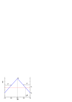
Figure 5: Sketch of the density profile in a cylindric volume $V=\pi R^{2}L_{z}$ for a non-absorbing boundary. Without forces the system relaxes to a homogeneous state with $n=n_{h}$ where $n_{\scriptscriptstyle R}<n_{h}<n_{0}$.

The density $n_{h}$ can be calculated in the following manner. The total number of particles in the volume $V$ is again given by Eq. (4). In the relaxed state, both the total number of particles and volume remain the same, so $N=n_{h}V$ and this directly yields

$$n_{h}=\frac{n_{0}}{3}+\frac{2n_{\scriptscriptstyle R}}{3}.$$

The intersection of the lines $n=n(r)$ and $n=n_{h}$ is at $r_{c}=2R/3$ and this remains so for any $n_{0}$ and $n_{\scriptscriptstyle R}$. At $t\rightarrow\infty$ the internal energy will reduce to the thermal energy (5). In any other moment it will be the sum of the internal energy (5) and potential energy $\Sigma_{p}$ with respect to the density level $n_{h}$. The potential energy is the sum of the two integrals $\Sigma_{p}=\Sigma_{p1}+\Sigma_{p2}$,

$$\Sigma_{p1}=\kappa T\int_{0}^{r_{c}}[n(r)-n_{h}]dV,\quad\Sigma_{p2}=\kappa T\int_{r_{c}}^{R}[n_{h}-n(r)]dV.$$

The result turns out to be

$$\Sigma_{p1}=\Sigma_{p2}=\frac{8}{81}V\kappa T(n_{0}-n_{\scriptscriptstyle R}),$$

so that

$$\Sigma_{p}=\frac{16}{81}V\kappa T(n_{0}-n_{\scriptscriptstyle R}).$$ (13)

This may be compared with the potential energy (7) from the case of absorbing boundaries. The ratio of the two is $E_{p}/\Sigma_{p}\approx 1.7$. Such a result could have been foreseen because the reference level with respect to which the energy is calculated in the present case is higher, so the potential energy is naturally smaller.

It should be stressed that this is a completely general and exact analysis and it can be performed in the same manner for any other analytically given density profile. For example, the profile in Fig. 6 is in fact a function of the kind $c_{1}+\exp(-c_{2}r^{2})J_{0}(c_{3}r)$ (where $J_{0}$ is the Bessel function), but such derivations will not be repeated here.

Figure 6: Sketch of the two density profiles, linear and Gaussian, in a cylindric volume $V=\pi R^{2}L_{z}$, in balance with some radially acting force $\vec{F}$. Without forces the system relaxes to a homogeneous state with $n=n_{h}$.

IV Summary and conclusions

Inhomogeneity of plasmas implies a free energy for development of drift instabilities as the most efficient way of relaxing into a more favorable lower energy state. Such instabilities may be accompanied with stochastic heating provided large enough amplitudes of the perturbations, and this phenomenon has been observed in the past in specially designed laboratory experiments.(Hatakeyama et al., 1980; McChesney et al., 1987, 1991; Sanders et al., 1998)

The same idea has been used recently(Vranjes & Poedts, 2009a, b, c, d, 2010a, 2010b) as a new paradigm for the heating of the solar corona. Analytical calculations in these references show that such a stochastic heating can easily satisfy numerous heating requirements like the necessary heating rate, better heating of heavier particles, stronger heating in perpendicular direction with respect to the magnetic field vector, etc. The model is based on a quasi-static inhomogeneous background plasma which is supposed to contain enough energy in order for the mechanism to work. This assumption is checked in the present study, and the energy contained in the density gradient is calculated. The results obtained in the work suggest that accidentally and externally created magnetic structures indeed contain enough energy for a sustainable heating at least in the solar quiet regions and in coronal holes.

The inhomogeneity is an intrinsic feature of the magnetic structures in the solar atmosphere. Movement and restructuring is a continuous process in coronal magnetic structures and such phenomena are accompanied with the motion of plasma due to its frozen-in properties. The life-time of these structures is of the order of an hour, so that indeed they can be treated as quasi-static for relatively fast drift instabilities, and they are maintained by processes deep below the corona itself. This implies that such a drift-wave-favorable environment is being created continuously; structures appear and disappear all the time, and heating is taking place in each of them independently. As discussed in Vranjes & Poedts (2009a, b), the drift waves and heating are produced directly in these magnetic structures and driven by the plasma inhomogeneity. However, the complete mechanism is totally magnetic by nature: such inhomogeneities are caused by the dynamics and restructuring of the magnetic field, and these phenomena on the other hand are driven by processes far from the corona, i.e., inside the Sun. In the present work we were focused only on the heating rate close to the energy loss rate, to check if it can be sustainable or not. However various heating rates are possible dependent on the drift wave frequency and growth-rate (which on the other hand are dependent on the inhomogeneity scale-length), including energy releases in the range of nano-flares(Vranjes & Poedts, 2009c).

The analysis presented in the work is for a simple cylindric geometry, but it can easily be generalized to other geometries applicable to the laboratory plasma like a tokamak, or to loop structures in the solar atmosphere.

References

- Pandey & Vranjes (2005) B. P. Pandey and J. Vranjes, Phys. Scripta 72, 247 (2005).
- Cahn & Hilliard (1958) J. W. Chan and J. E. Hilliard, J. Chem. Phys. 28, 258 (1958).
- Hart (1959) E. W. Hart, Phys. Rev. 113, 412 (1959).
- Rice & Chang (1974) O. K. Rice and D. R. Chang, Physica 78, 500 (1974).
- Silver (1978) R. N. Silver, Phys. Rev. B 17, 3955 (1978).
- McCoy & Davis (1979) B. F. McCoy and H. T. Davis, Phys. Rev. A 20, 1201 (1979).
- Warner (1980) M. Warner, Chem. Phys. Lett. 70, 155 (1980).
- Lowett & Baus (1992) R. Lowett and M. Baus, Physica A 181, 309 (1992).
- Vranjes & Poedts (2009a) J. Vranjes and S. Poedts, MNRAS 398, 918 (2009a).
- Vranjes & Poedts (2009b) J. Vranjes and S. Poedts, MNRAS 400, 2147 (2009b).
- Vranjes & Poedts (2009c) J. Vranjes and S. Poedts, Phys. Plasmas 16, 092902 (2009c).
- Vranjes & Poedts (2009d) J. Vranjes and S. Poedts, EPL 86, 39001 (2009d).
- Vranjes & Poedts (2010a) J. Vranjes and S. Poedts, MNRAS 408, 1835 (2010a).
- Vranjes & Poedts (2010b) J. Vranjes and S. Poedts, Astrophys. J. 719, 1335 (2010b).
- Vranjes (2011) J. Vranjes, MNRAS 415, 1543 (2011).
- Vranjes (2011) J. Vranjes, A&A 532, A137 (2011).
- TRACE (2014) http://soi.stanford.edu/results/SolPhys200/Schrijver/TRACEpod_archive.html
- Wikipedia (2014) Wikipedia contributors. “Arcus cloud.” Wikipedia, The Free Encyclopedia. Wikipedia, The Free Encyclopedia, 1 Jun. 2014. Web. 19 Sep. 2014.
- Wikipedia (2014) Wikipedia contributors. “Morning Glory cloud.” Wikipedia, The Free Encyclopedia. Wikipedia, The Free Encyclopedia, 30 Aug. 2014. Web. 19 Sep. 2014.
- Smith (1988) R. K. Smith, Earth Sci. Rev. 25, 267 (1988).
- Rottman & Grimshaw (2004) J. W. Rottman and R. Grimshaw, in Environmental stratified flows, ed. R. Grimshaw (Kluver, Dordrecht, 2003).
- Goler & Reeder (2004) R. A. Goler and M. J. Reeder, J. Atmos. Sci. 61, 1360 (2004).
- Hartung & Sitkowski (2010) D. C. Hartung and M. Sitkowski, Weather 65, 148 (2010).
- Hatakeyama et al. (1980) R. Hatakeyama, M. Oertl, E. Märk, and R. Schrittwieser, Phys. Fluids 23, 1774 (1980).
- McChesney et al. (1987) J. M. McChesney, R. A. Stern, and P. M. Bellan, Phys. Rev. Lett. 59, 1436 (1987).
- McChesney et al. (1991) J. M. McChesney, P. M. Bellan, and R. A. Stern, Phys. Fluids B 3, 3363 (1991).
- Sanders et al. (1998) S. J. Sanders, P. M. Bellan, and R. A. Stern, Phys. Plasmas 5, 716 (1998).
- Narain & Ulmschenider (1990) U. Narain and P. Ulmschneider, Space. Sci. Rev. 54, 377 (1990).