Wigner Distributions for Gluons in Light-front Dressed Quark Model

Abstract

We present a calculation of Wigner distributions for gluons in light-front dressed quark model. We calculate the kinetic and canonical gluon orbital angular momentum and spin-orbit correlation of the gluons in this model.

I Introduction

To have a complete understanding of matter at subatomic level, it is important to understand the nucleon spin structure. This means an understanding of how the spin ($\frac{1}{2}$) of the nucleon is shared by the quarks and gluons in the nucleon and what is the contribution of their orbital angular momentum (OAM). Earlier it was believed that all nucleon spin is carried by quarks. EMC experiment showed that contribution of quark spin to nucleon spin is very small. So, an important question is from where does the missing (remaining) angular momentum comes from? As the nucleon is made up of quarks and gluons, it is natural to expect that the missing angular momentum come either from gluon spin or from quark or gluon OAM. This is expressed by spin sum rule jm

$$\frac{1}{2}=\frac{1}{2}\sum_{q}{\Delta q}+\underbrace{\sum_{q}\mathcal{L}^{q}}_{\text{quark OAM}}+\Delta G+\underbrace{{\mathcal{L}^{g}}}_{\text{Gluon OAM}}$$

Here $\frac{1}{2}\sum_{q}{\Delta q}$ and $\Delta G$ are quark and gluon spin angular momentum respectively. The above sum rule is called canonical spin sum rule. Except quark intrinsic part, other terms depend upon specific gauge choice.

Recently, Chen et al chen introduced a gauge invariant extension (GIE) which is basically a prescription to find a manifestly gauge invariant quantity that coincides with a gauge non-invariant quantity in a particular gauge. In this way, one can extend the validity of a physical interpretation of the canonical OAM $\mathcal{L}^{q}$ and $\mathcal{L}^{g}$ in light front gauge to any other gauge. There is another decomposition called kinetic decomposition of nucleon spin ji1

$$\frac{1}{2}=S^{q}+L^{q}+J^{g}$$

where $S^{q}$ and $L^{q}$ are quark spin and kinetic orbital angular momentum respectively. $J^{g}$ is total gluon contribution to the angular momentum of nucleon. Later, Wakamatsu wak further separated the $J^{g}$ into a gluon orbital part ($L^{g}$) and an intrinsic part ($S^{g}$) using a prescription similar to chen . Which of the two definitions of the OAM is ”physical” is a matter of intense debate. According to the current understanding the difference between kinetic and canonical OAM is the choice of the Wilson line in the definition of non-local quark operator: a staple type gauge link gives canonical OAM whereas a straight line gauge gives kinetic OAM. Interesting physical interpretation of both type of OAM is given in OAM_rev ; mb

Recently it has been shown that the Wigner distribution can provide useful information on the spin and angular momentum correlation of quarks and gluons in the nucleon. Wigner distributions wigner are quasi-probabilistic distribution in which both position and momentum space information are encoded. They are directly related to generalized parton correlation functions (GPCFs) metz . GPCFs are fully unintegrated off-diagonal quark-quark correlator and contain maximum amount of information about the structure of nucleon. If we integrate GPCFs over light cone energy ($k^{-}$), we get generalized transverse momentum dependent parton distribution functions (GTMDs). These GTMDs are Fourier transform of Wigner distributions and vice versa.

In fact, the GTMDs are directly related to generalized parton distributions (GPDs) ji1 and transverse momentum dependent parton distribution functions (TMDs) metz , both of which have been found to give very useful information about the structure and spin of the nucleon in terms of quarks and gluons. We can take two-dimensional Fourier transform of GPDs with respect to the momentum transfer in the transverse direction to get impact parameter dependent parton distribution functions (IPDPDFs) burkardt . These give the correlation in transverse position and longitudinal momentum for different quark and target polarization. On the other hand, TMDs provide momentum space information, and also the strength of spin-orbit and spin-spin correlation. It has been shown that both of these distributions are linked to GTMDs. So we can consider the GTMDs, or equivalently Wigner distribution as mother distributions.

Wigner distributions described above, are joint position and momentum space distributions of quarks and gluons in the nucleon. Due to uncertainty principle, they are not positive definite and do not have probabilistic interpretation. However, integration of Wigner distributions over one or more variables relates them to measurable quantities lorce . Here model calculation of Wigner functions are important as these calculations play a significant role in revealing what kind of information they can provide about the correlations of quarks and gluons inside the nucleon. Also such calculations are useful to check various relations among the GTMDs and the TMDs and GPDs. In fact some relations have been found to hold only in certain class of models metz1 . In this work, we calculate the Wigner distributions in light front Hamiltonian approach pedestrian . This approach gives a intuitive picture of deep inelastic scattering processes, as it is based on field theory but keeps close contact with parton ideas kundu1 . Here the partons i.e quarks and gluons are non-collinear, massive and they also interact. The target state is expanded in Fock space in terms of multi-parton light front wave functions (LFWFs). The advantage of using light front (infinite momentum frame) formalism is that such wave functions are boost invariant, so one can work with a finite number of constituents of the nucleon and this picture is invariant under Lorentz boost brod1 . In order to obtain the LFWFs of the nucleon, one needs a model light front Hamiltonian. However many useful information can be obtained if one replaces the bound state by a simple spin-$\frac{1}{2}$ composite relativistic state like a quark at one loop dressed with a gluon hadron_optics1 ; hadron_optics2 . In our previous work our1 , we studied the Wigner distribution of quarks for a simple relativistic spin-$\frac{1}{2}$ composite system, namely for a quark dressed with a gluon, using light front Hamiltonian perturbation theory. Here we calculate the Wigner distribution for gluons in the same model. This calculation is useful as in most phenomenological models commonly studied, gluonic degrees of freedom are not present lorce , and a study of the gluon spin and OAM is not possible there.

II Wigner Distributions

The Wigner distribution for gluons can be defined as Jifeng

$$xW^{g}(x,\vec{k}_{\perp},\vec{b}_{\perp})=\int\frac{d^{2}\vec{\Delta}_{\perp}}{(2\pi)^{2}}e^{-i\vec{\Delta}_{\perp}.\vec{b}_{\perp}}\int\frac{dz^{-}d^{2}z_{\perp}}{2(2\pi)^{3}p^{+}}e^{ik.z}$$

$$\Big{\langle}p^{+},\frac{\vec{\Delta}_{\perp}}{2},\sigma\Big{|}\Gamma^{ij}F^{+i}\Big{(}-\frac{z}{2}\Big{)}F^{+j}\Big{(}\frac{z}{2}\Big{)}\Big{|}p^{+},-\frac{\vec{\Delta}_{\perp}}{2},\sigma\Big{\rangle}\Big{|}_{z^{+}=0};$$ (1)

where $\vec{\Delta}_{\perp}$ is the transverse momentum transfer from the target state and $\vec{b}_{\perp}$ is 2 dimensional vector in impact parameter space conjugate to $\vec{\Delta}_{\perp}$. We calculate Eq. (1) for $\Gamma^{ij}=\delta^{ij}$ and $\Gamma^{ij}=-i\epsilon^{ij}_{\perp}$.

We have,

$$F^{+i}=\partial^{+}A^{i}-\partial^{i}A^{+}+gf^{abc}A^{+}A^{i}.$$

The gauge field can be written as kundu1 , for $i=1,2$,

$$A^{i}\Big{(}\frac{z}{2}\Big{)}=\sum_{\lambda}\int\frac{dk^{+}d^{2}k_{\perp}}{2k^{+}(2\pi)^{3}}\Big{[}\epsilon_{\lambda}^{i}(k)a_{\lambda}(k)e^{-\frac{i}{2}k.z}+\epsilon_{\lambda}^{*i}(k)a^{\dagger}_{\lambda}(k)e^{\frac{i}{2}k.z}\Big{]}.$$

We choose the light front gauge, $A^{+}=0$, and take the gauge link to be unity.

In our previous work our1 we calculated the quark Wigner distributions for a quark state dressed with a gluon. In this work we investigate the gluon Wigner distribution in the same model using light-front Hamiltonian perturbation theory. The state can be expanded in Fock space in terms of multi-parton light-front wave functions (LFWFs) as hari

$$\Big{|}p^{+},p_{\perp},\sigma\Big{\rangle}=\Phi^{\sigma}(p)b^{\dagger}_{\sigma}(p)|0\rangle+\sum_{\sigma_{1}\sigma_{2}}\int[dp_{1}]\int[dp_{2}]\sqrt{16\pi^{3}p^{+}}\delta^{3}(p-p_{1}-p_{2})$$

$$\Phi^{\sigma}_{\sigma_{1}\sigma_{2}}(p;p_{1},p_{2})b^{\dagger}_{\sigma_{1}}(p_{1})a^{\dagger}_{\sigma_{2}}(p_{2})|0\rangle;$$ (2)

where $[dp]=\frac{dp^{+}d^{2}p_{\perp}}{\sqrt{16\pi^{3}p^{+}}}$ and $\sigma_{1}$ and $\sigma_{2}$ are the helicities of the quark and gluon respectively. The LFWFs ($\Phi^{\sigma}(p)$ and $\Phi^{\sigma}_{\sigma_{1}\sigma_{2}}$) appearing in Eq. (II) are calculated by solving the light-front eigenvalue equation in the Hamiltonian approach. $\Phi^{\sigma}(p)$ is the single particle (quark) LFWF gives the wave function re-normalization for the quark and $\Phi^{\sigma}_{\sigma_{1}\sigma_{2}}$ is the two particle (quark-gluon) LFWF. $\Phi^{\sigma}_{\sigma_{1}\sigma_{2}}(p;p_{1},p_{2})$ gives the probability amplitude to find a bare quark having momentum $p_{1}$ and helicity $\sigma_{1}$ and a bare gluon with momentum $p_{2}$ and helicity $\sigma_{2}$ in the dressed quark. The two particle LFWF is related to the boost invariant LFWF; $\Psi^{\sigma}_{\sigma_{1}\sigma_{2}}(x,q_{\perp})=\Phi^{\sigma}_{\sigma_{1}\sigma_{2}}\sqrt{p^{+}}$. Here we have used the Jacobi momenta $(x_{i},q_{i\perp})$ :

$$p_{i}^{+}=x_{i}p^{+},~{}~{}~{}~{}~{}~{}~{}~{}~{}~{}q_{i\perp}=k_{i\perp}+x_{i}p_{\perp};$$ (3)

so that $\sum_{i}x_{i}=1,\sum_{i}q_{i\perp}=0$. These two-particle LFWFs can be calculated perturbatively as hari :

$$\Psi^{\sigma a}_{\sigma_{1}\sigma_{2}}(x,q_{\perp})=\frac{1}{\Big{[}m^{2}-\frac{m^{2}+(q_{\perp})^{2}}{x}-\frac{(q_{\perp})^{2}}{1-x}\Big{]}}\frac{g}{\sqrt{2(2\pi)^{3}}}T^{a}\chi^{\dagger}_{\sigma_{1}}\frac{1}{\sqrt{1-x}}$$

$$\Big{[}-2\frac{q_{\perp}}{1-x}-\frac{(\sigma_{\perp}.q_{\perp})\sigma_{\perp}}{x}+\frac{im\sigma_{\perp}(1-x)}{x}\Big{]}\chi_{\sigma}(\epsilon_{\perp\sigma_{2}})^{*}.$$ (4)

We use the two component formalism zhang . $\chi$ is the two component fermion spinor. $T^{a}$ are the usual color $SU(3)$ matrices, $m$ is the mass of the quark and $\epsilon_{\perp\sigma_{2}}$ is the polarization vector of the gluon.

The gluon-gluon correlator in Eq. (1) for a quark state dressed with a gluon can be expressed in terms of the overlap of two-particle LFWFs. The single particle sector of the Fock space expansion contributes only at $x=1$ and we exclude this.

For $\Gamma^{ij}=\delta^{ij}$ we get

$$W^{\sigma\sigma^{\prime}}_{1}(x,k_{\perp},b_{\perp})=-\sum_{\sigma_{1},\sigma_{2},\lambda_{1}}\int\frac{d^{2}\Delta_{\perp}}{2(2\pi)^{2}}e^{-i\Delta_{\perp}.b_{\perp}}\Bigg{[}\Psi^{*\sigma^{\prime}}_{\sigma_{1}\lambda_{1}}(\hat{x},\hat{q}^{\prime}_{\perp})\Psi^{\sigma}_{\sigma_{1}\sigma_{2}}(\hat{x},\hat{q}_{\perp})\Big{(}\epsilon_{\sigma_{2}}^{1}\epsilon_{\lambda_{1}}^{*1}+\epsilon_{\sigma_{2}}^{2}\epsilon_{\lambda_{1}}^{*2}\Big{)}\Bigg{]};$$ (5)

and for $\Gamma^{ij}=-i\epsilon^{ij}_{\perp}$ we get

$$W^{\sigma\sigma^{\prime}}_{2}(x,k_{\perp},b_{\perp})=-i\sum_{\sigma_{1},\sigma_{2},\lambda_{1}}\int\frac{d^{2}\Delta_{\perp}}{2(2\pi)^{2}}e^{-i\Delta_{\perp}.b_{\perp}}\Bigg{[}\Psi^{*\sigma^{\prime}}_{\sigma_{1}\lambda_{1}}(\hat{x},\hat{q}^{\prime}_{\perp})\Psi^{\sigma}_{\sigma_{1}\sigma_{2}}(\hat{x},\hat{q}_{\perp})\Big{(}\epsilon_{\sigma_{2}}^{1}\epsilon_{\lambda_{1}}^{*2}-\epsilon_{\sigma_{2}}^{2}\epsilon_{\lambda_{1}}^{*1}\Big{)}\Bigg{]};$$ (6)

where $\hat{x}=(1-x)$ and $\hat{q}_{\perp}=-q_{\perp}$. Jacobi relation for the transverse momenta in the symmetric frame is given by $q^{\prime}_{\perp}=k_{\perp}-\frac{\Delta_{\perp}}{2}(1-x)$ and $q_{\perp}=k_{\perp}+\frac{\Delta_{\perp}}{2}(1-x)$. We represent the gluon Wigner distribution as $W^{\lambda\lambda^{\prime}}$, where $\lambda$ and $\lambda^{\prime}$ are polarization of target state and gluon respectively.

We consider only longitudinally polarized target state and then we have four gluon Wigner distributions as follows, in a manner similar to quark Wigner distributions lorce

Wigner distribution of unpolarized gluon in unpolarized target state as

$$W^{UU}=W^{\uparrow\uparrow}_{1}(x,k_{\perp},b_{\perp})+W^{\downarrow\downarrow}_{1}(x,k_{\perp},b_{\perp});$$ (7)

Wigner distribution corresponding to the distortion due to longitudinal polarization of the target as

$$W^{LU}=W^{\uparrow\uparrow}_{1}(x,k_{\perp},b_{\perp})-W^{\downarrow\downarrow}_{1}(x,k_{\perp},b_{\perp});$$ (8)

Wigner distribution corresponding to the distortion due to longitudinal polarization of the gluons as

$$W^{UL}=W^{\uparrow\uparrow}_{2}(x,k_{\perp},b_{\perp})+W^{\downarrow\downarrow}_{2}(x,k_{\perp},b_{\perp});$$ (9)

and the Wigner distribution corresponding to the correlation due to longitudinal polarization of the target state and the gluons

$$W^{LL}=W^{\uparrow\uparrow}_{2}(x,k_{\perp},b_{\perp})-W^{\downarrow\downarrow}_{2}(x,k_{\perp},b_{\perp}).$$ (10)

The final expressions for these four gluon Wigner distributions are given by, using the two-particle LFWFs

$$W^{UU}(x,k_{\perp},b_{\perp})=N\int d\Delta_{x}\int d\Delta_{y}\frac{\mathrm{cos}(\Delta_{\perp}\cdot b_{\perp})}{D(q_{\perp})D(q^{\prime}_{\perp})}\Big{[}\frac{-4\Big{(}(q_{\perp}q^{\prime}_{\perp})(x^{2}-2x+2)+m^{2}x^{4}\Big{)}}{x^{3}(x-1)^{2}}\Big{]};$$ (11)

$$W^{LU}(x,k_{\perp},b_{\perp})=N\int d\Delta_{x}\int d\Delta_{y}\frac{\mathrm{sin}(\Delta_{\perp}\cdot b_{\perp})}{D(q_{\perp})D(q^{\prime}_{\perp})}\Big{[}\frac{4(2-x)(q_{2}q^{\prime}_{1}-q_{1}q^{\prime}_{2})}{x^{2}(x-1)^{2}}\Big{]};$$ (12)

$$W^{UL}(x,k_{\perp},b_{\perp})=N\int d\Delta_{x}\int d\Delta_{y}\frac{\mathrm{sin}(\Delta_{\perp}\cdot b_{\perp})}{D(q_{\perp})D(q^{\prime}_{\perp})}\Big{[}\frac{4(x^{2}-2x+2)(q_{2}q^{\prime}_{1}-q_{1}q^{\prime}_{2})}{x^{3}(x-1)^{2}}\Big{]};$$ (13)

$$W^{LL}(x,k_{\perp},b_{\perp})=N\int d\Delta_{x}\int d\Delta_{y}\frac{\mathrm{cos}(\Delta_{\perp}\cdot b_{\perp})}{D(q_{\perp})D(q^{\prime}_{\perp})}\Big{[}\frac{4\Big{(}(q_{\perp}q^{\prime}_{\perp})(2-x)+m^{2}x^{3}\Big{)}}{x^{2}(x-1)^{2}}\Big{]};$$ (14)

where $A_{x},A_{y}$ are $x,y$ component of $A_{\perp}$ and

$$D(k_{\perp})=\Big{(}m^{2}-\frac{m^{2}+(k_{\perp})^{2}}{1-x}-\frac{(k_{\perp})^{2}}{x}\Big{)}\hskip 14.22636pt,\hskip 14.22636ptN=\frac{g^{2}}{2(2\pi)^{2}}.$$

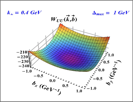
(a)    (b)

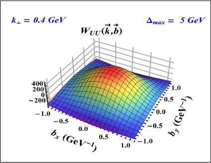
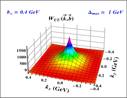
(c)    (d)

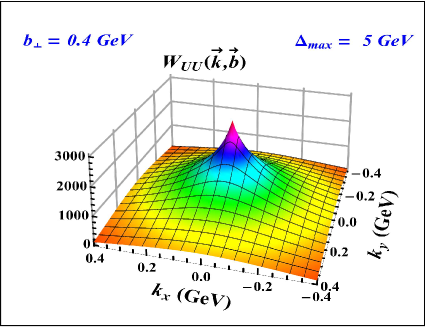
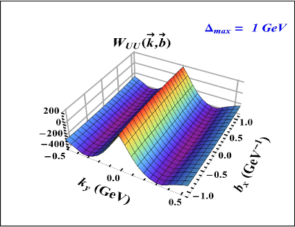
(e)    (f)

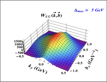
Figure 1: (Color online) 3D plots of the Wigner distributions $W^{UU}$. Plots (a) and (b) are in $b$ space with $k_{\perp}=0.4$ GeV. Plots (c) and (d) are in $k$ space with $b_{\perp}=0.4$ $\mathrm{GeV}^{-1}$. Plots (e) and (f) are in mixed space where $k_{x}$ and $b_{y}$ are integrated. All the plots on the left panel (a,c,e) are for $\Delta_{max}=1.0$ GeV. Plots on the right panel (b,d,f) are for $\Delta_{max}=5.0$ GeV. For all the plots we kept $m=0.33$ GeV, integrated out the $x$ variable and we took $\vec{k_{\perp}}=k\hat{j}$ and $\vec{b_{\perp}}=b\hat{j}$.

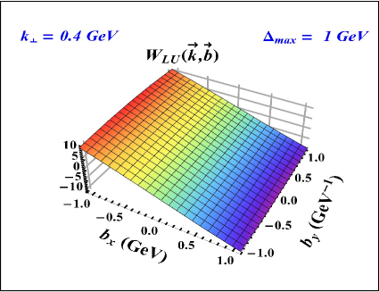
(a)    (b)

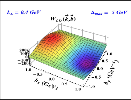
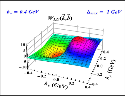
(c)    (d)

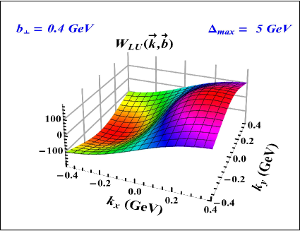
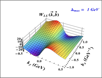
(e)    (f)

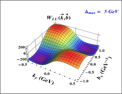
Figure 2: (Color online) 3D plots of the Wigner distributions $W^{LU}$. Plots (a) and (b) are in $b$ space with $k_{\perp}=0.4$ GeV. Plots (c) and (d) are in $k$ space with $b_{\perp}=0.4$ $\mathrm{GeV}^{-1}$. Plots (e) and (f) are in mixed space where $k_{x}$ and $b_{y}$ are integrated. All the plots on the left panel (a,c,e) are for $\Delta_{max}=1.0$ GeV. Plots on the right panel (b,d,f) are for $\Delta_{max}=5.0$ GeV. For all the plots we kept $m=0.33$ GeV, integrated out the $x$ variable and we took $\vec{k_{\perp}}=k\hat{j}$ and $\vec{b_{\perp}}=b\hat{j}$.

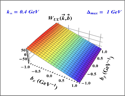
(a)    (b)

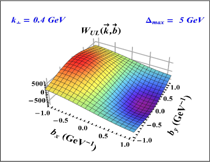
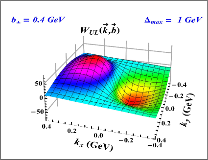
(c)    (d)

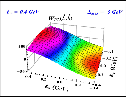
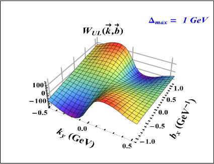
(e)    (f)

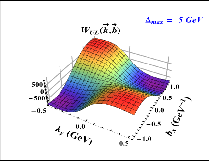
Figure 3: (Color online) 3D plots of the Wigner distributions $W^{UL}$. Plots (a) and (b) are in $b$ space with $k_{\perp}=0.4$ GeV. Plots (c) and (d) are in $k$ space with $b_{\perp}=0.4$ $\mathrm{GeV}^{-1}$. Plots (e) and (f) are in mixed space where $k_{x}$ and $b_{y}$ are integrated. All the plots on the left panel (a,c,e) are for $\Delta_{max}=1.0$ GeV. Plots on the right panel (b,d,f) are for $\Delta_{max}=5.0$ GeV. For all the plots we kept $m=0.33$ GeV, integrated out the $x$ variable and we took $\vec{k_{\perp}}=k\hat{j}$ and $\vec{b_{\perp}}=b\hat{j}$.

(a)    (b)

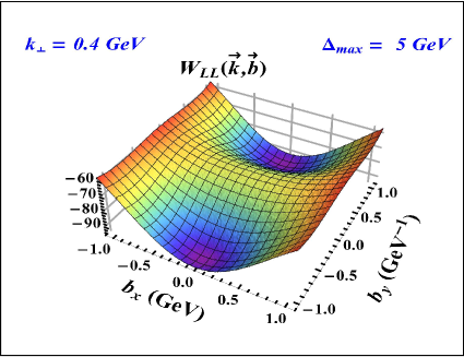
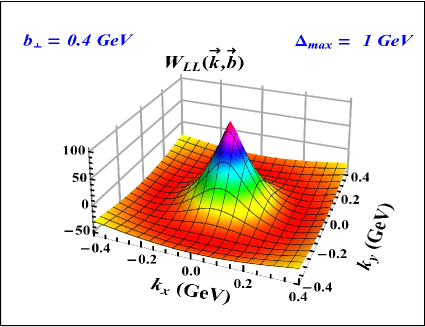
(c)    (d)

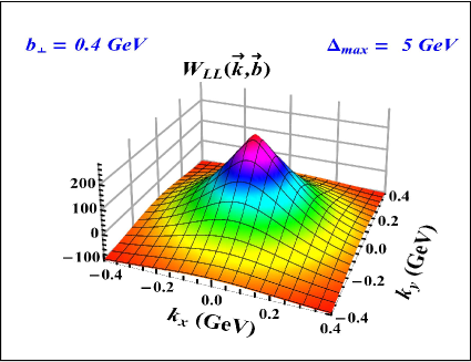
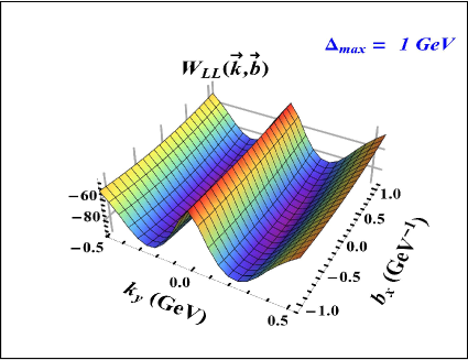
(e)    (f)

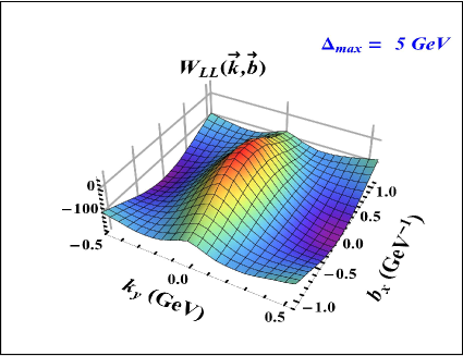
Figure 4: (Color online) 3D plots of the Wigner distributions $W^{LL}$. Plots (a) and (b) are in $b$ space with $k_{\perp}=0.4$ GeV. Plots (c) and (d) are in $k$ space with $b_{\perp}=0.4$ $\mathrm{GeV}^{-1}$. Plots (e) and (f) are in mixed space where $k_{x}$ and $b_{y}$ are integrated. All the plots on the left panel (a,c,e) are for $\Delta_{max}=1.0$ GeV. Plots on the right panel (b,d,f) are for $\Delta_{max}=5.0$ GeV. For all the plots we kept $m=0.33$ GeV, integrated out the $x$ variable and we took $\vec{k_{\perp}}=k\hat{j}$ and $\vec{b_{\perp}}=b\hat{j}$.

III Gluon GTMDs and Orbital Angular Momentum

In order to calculate the gluon GTMDs we use the parametrization as shown in gluon_gtmd where the authors have shown that the correlators like in Eq. (1) can in general be written as

$$W^{\it{O}}_{\Lambda^{\prime},\Lambda}=\int\frac{dz^{-}d^{2}z_{\perp}}{2(2\pi)^{3}}e^{i\frac{xP^{+}}{2}z^{-}-i\vec{k}_{\perp}.\vec{z}_{\perp}}\langle p^{\prime},\Lambda^{\prime}\mid O(z)\mid p,\Lambda\rangle=\bar{u}(p^{\prime},\Lambda^{\prime})M^{O}u(p,\Lambda);$$ (15)

where $O(z)$ stands for the relevant quark or gluon operators and $M^{O}$ stands for the matrix in Dirac space with $O$ determined by the corresponding quark or gluon operator. The amplitude shown in Eq. (15) takes the following generic structure when the momentum transfer is purely in the transverse direction :

$$W^{\Delta S_{z},c_{P}}_{\Lambda^{\prime},\Lambda}=\frac{\bar{u}(p^{\prime},\Lambda^{\prime})M^{\Delta S_{z},c_{P}}u(p,\Lambda)}{2P^{+}};$$ (16)

where $c_{P}$ is the parity coefficient of the partonic operator and $\Delta S_{z}$ is the spin flip number given by $\Delta S_{z}=\lambda^{\prime}-\lambda+\Delta L_{z}$ such that $\lambda(\lambda^{\prime})$ is the initial (final) parton light front helicity and $\Delta L_{z}$ is the eigenvalue of the operator $\Delta\hat{L}_{z}=\hat{L}_{z}-\hat{L^{\prime}}_{z}$. Also for twist-2 partonic operators we get $\Delta L_{z}=0$ and hence $\Delta S_{z}=\lambda^{\prime}-\lambda$.

The gluon operators appearing in Eq. (1) corresponds to the case when $\Delta S_{z}=0$ and $c_{P}=\pm 1$ as shown in eq (3.12), eq (3.42) and eq (3.43) of Eq. (17). So the relevant parameterization of the gluon GTMDs which correspond to $\Gamma^{ij}=\delta^{ij}$ in Eq. (1) is:

$$M^{0,+}=\Big{(}\frac{M}{P^{+}}\Big{)}^{t-1}\Big{[}\gamma^{+}\Big{(}S^{0,+}_{t,ia}+\gamma_{5}\frac{i\epsilon_{T}^{k_{T}\Delta_{T}}}{M^{2}}S^{0,+}_{t,ib}\Big{)}+i\sigma^{j+}\Big{(}\frac{k_{T}^{j}}{M}P^{0,+}_{t,ia}+\frac{\Delta_{T}^{j}}{M}P^{0,+}_{t,ib}\Big{)}\Big{]};$$ (17)

where

$$\epsilon_{T}^{ab} = \epsilon_{T}^{ij}a^{i}b^{j};$$

$$\epsilon_{T}^{ij} = \epsilon^{-+12}=+1.$$

t+1 is defined as the twist of the operator in gluon_gtmd , so for twist 2 we take $t=1$.
Comparing and solving Eq. (1) and Eq. (16), we get the following expression for the gluon GTMDs:

$$S^{0,+}_{1,ia} = \frac{-2N}{D(q_{\perp})D(q^{\prime}_{\perp})}\Bigg{[}\frac{m^{2}x^{4}+k_{\perp}^{2}(x^{2}-2x+2)}{x^{3}(x-1)^{2}}-\frac{\Delta_{\perp}^{2}(x^{2}-2x+2)}{4x^{3}}\Bigg{]};$$

$$S^{0,+}_{1,ib} = \frac{2N}{D(q_{\perp})D(q^{\prime}_{\perp})}\Bigg{[}\frac{m^{2}(2-x)}{(1-x)x^{2}}\Bigg{]};$$

$$P^{0,+}_{1,ia} = \frac{2N}{D(q_{\perp})D(q^{\prime}_{\perp})}\Bigg{[}\frac{m^{2}\Delta_{\perp}^{2}}{x(k_{2}\Delta_{1}-k_{1}\Delta_{2})}\Bigg{]};$$

$$P^{0,+}_{1,ib} = \frac{2N}{D(q_{\perp})D(q^{\prime}_{\perp})}\Bigg{[}\frac{-m^{2}(k_{\perp}.\Delta_{\perp})}{x(k_{2}\Delta_{1}-k_{1}\Delta_{2})}\Bigg{]}.$$ (18)

The relations of these GTMDs with that in metz are:-

$$S^{0,+}_{1,ia} = F_{1,1}^{g};$$

$$S^{0,+}_{1,ib} = F_{1,4}^{g};$$

$$P^{0,+}_{1,ia} = F_{1,2}^{g};$$

$$P^{0,+}_{1,ib} = -\frac{F_{1,1}^{g}}{2}+F_{1,3}^{g}.$$

So for the gluon case we get $F_{1,4}^{g}$ as shown below and this relation agrees with that in other .

$$F_{1,4}^{g}=\frac{N}{D(q_{\perp})D(q^{\prime}_{\perp})}\Bigg{[}\frac{m^{2}(2-x)}{(1-x)x^{2}}\Bigg{]}.$$ (20)

From this, we can calculate the gluon canonical OAM since the canonical OAM is related to the GTMD $F_{1,4}$ as follows, similar to quarks lorce ; OAM3 ; hatta1

$$l^{g}_{z}=-\int dxd^{2}k_{\perp}\frac{k_{\perp}^{2}}{m^{2}}F_{1,4}^{g}.$$ (21)

This gives,

$$l^{g}_{z}=-N\int dx(1-x)(2-x)\Big{[}I_{1}-m^{2}x^{2}I_{2}\Big{]};$$ (22)

where,

$$I_{1} =\int\frac{d^{2}k_{\perp}}{m^{2}x^{2}+(k_{\perp})^{2}}=\pi log\Bigg{[}\frac{Q^{2}+m^{2}x^{2}}{\mu^{2}+m^{2}x^{2}}\Bigg{]};$$

$$I_{2} =\int\frac{d^{2}k_{\perp}}{\Big{(}m^{2}x^{2}+(k_{\perp})^{2}\Big{)}^{2}}=\frac{\pi}{(m^{2}x^{2})};$$

Here $Q$ and $\mu$ are the upper and lower limits of the $k_{\perp}$ integration respectively.

For the case when $\Delta S_{z}=0$ and $c_{P}=-1$ which corresponds to $\Gamma^{ij}=-i\epsilon^{ij}_{\perp}$ in Eq. (1) the relevant gluon parameterization is given by gluon_gtmd :

$$M^{0,-}=\Big{(}\frac{M}{P^{+}}\Big{)}^{t-1}\Big{[}\gamma^{+}\gamma_{5}\Big{(}S^{0,-}_{t,ia}+\gamma_{5}\frac{i\epsilon_{T}^{k_{T}\Delta_{T}}}{M^{2}}S^{0,-}_{t,ib}\Big{)}+i\sigma^{j+}\gamma_{5}\Big{(}\frac{k_{T}^{j}}{M}P^{0,-}_{t,ia}+\frac{\Delta_{T}^{j}}{M}P^{0,-}_{t,ib}\Big{)}\Big{]}.$$ (23)

Again by solving Eq. (23) and Eq. (1) we get the corresponding GTMDs at twist two.

$$S^{0,-}_{1,ia} = \frac{N}{D(q_{\perp})D(q^{\prime}_{\perp})}\Bigg{[}\frac{4k_{\perp}^{2}(x-2)}{2(x-1)^{2}x^{2}}+\frac{\Delta_{\perp}^{2}}{(x-1)^{2}x^{2}}-\frac{4m^{2}x^{2}+\Delta_{\perp}^{2}(x^{2}-4x+5)}{2(x-1)^{2}x}\Bigg{]};$$

$$S^{0,-}_{1,ib} = \frac{N}{D(q_{\perp})D(q^{\prime}_{\perp})}\Bigg{[}\frac{2(x^{2}-2x+2)m^{2}}{x^{3}(1-x)}\Bigg{]};$$

$$P^{0,-}_{1,ia} = \frac{N}{D(q_{\perp})D(q^{\prime}_{\perp})}\Bigg{[}\frac{4(k_{\perp}.\Delta_{\perp})m^{2}}{x(x-1)(k_{2}\Delta_{1}-k_{1}\Delta_{2})}\Bigg{]};$$

$$P^{0,-}_{1,ib} = \frac{N}{D(q_{\perp})D(q^{\prime}_{\perp})}\Bigg{[}\frac{4k_{\perp}^{2}m^{2}}{x(x-1)(k_{1}\Delta_{2}-k_{2}\Delta_{1})}\Bigg{]}.$$ (24)

The relation of these GTMDs with that in metz can be written as :

$$S^{0,-}_{1,ia} = 2G_{1,4}^{g};$$

$$S^{0,-}_{1,ib} = -G_{1,1}^{g};$$

$$P^{0,-}_{1,ia} = \frac{2m^{2}G_{1,2}^{g}-\Delta_{\perp}^{2}G_{1,1}^{g}}{2m^{2}};$$

$$P^{0,-}_{1,ib} = \frac{2m^{2}G_{1,3}^{g}+k_{\perp}.\Delta_{\perp}G_{1,1}^{g}}{2m^{2}}.$$

The spin-orbit correlation factor for the gluons $C_{z}^{g}$ can be defined in terms of the GTMD $G_{1,1}^{g}$ as follows other , similar to quark case lorce_14

$$C_{z}^{g}=\int dxd^{2}k_{\perp}\frac{k_{\perp}^{2}}{m^{2}}G_{1,1}^{g}.$$ (26)

The GTMD $G_{1,1}^{g}$ calculated using Eq. (LABEL:re2) agrees with that in other :

$$G_{1,1}^{g}=-\frac{N}{D(q_{\perp})D(q^{\prime}_{\perp})}\Bigg{[}\frac{2(x^{2}-2x+2)m^{2}}{x^{3}(1-x)}\Bigg{]};$$ (27)

So the spin-orbit correlation factor for the gluons in the dressed quark model is given by :

$$C_{z}^{g}=-N\int dx\frac{2(x^{2}-2x+2)(1-x)}{x}\Big{[}I_{1}-m^{2}x^{2}I_{2}\Big{]}.$$ (28)

The kinetic OAM for the gluons can be calculated using the sum rule for the gluon GPD’s Ji :

$$L^{g}_{z}=\frac{1}{2}\int dx\{x[H^{g}(x,0,0)+E^{g}(x,0,0)]-\tilde{H^{g}}(x,0,0)\}.$$

The gluon GPDs in the above relation can be related to the GTMDs as follows:-

$$H^{g}(x,0,t) =\int d^{2}k_{\perp}F_{1,1}^{g};$$ (29)

$$E^{g}(x,0,t) =\int d^{2}k_{\perp}\Big{[}-F_{1,1}^{g}+2\Big{(}\frac{k_{\perp}.\Delta_{\perp}}{\Delta_{\perp}^{2}}F_{1,2}^{g}+F_{1,3}^{g}\Big{)}\Big{]};$$ (30)

$$\tilde{H}^{g}(x,0,t) =\int d^{2}k_{\perp}G_{1,4}^{g}.$$ (31)

Using the above relation and the gluon GTMD calculated above, we can write the kinetic gluon OAM in the dressed quark model as

$$L^{g}_{z}=\frac{N}{2}\int dx\Big{\{}-f(x)I_{1}+2\pi(1-x)\Big{\}};$$ (32)

where,

$$I_{1} =\int\frac{d^{2}k_{\perp}}{m^{2}x^{2}+(k_{\perp})^{2}}=\pi log\Bigg{[}\frac{Q^{2}+m^{2}x^{2}}{\mu^{2}+m^{2}x^{2}}\Bigg{]};$$

$$f(x) =2x^{2}-3x+2.$$

Unlike for the quarks our1 , canonical gluon OAM and and spin-orbit correlations are different in this model. Note that the GTMDs $F_{1,4}$ and $G_{1,1}$ depend on the gauge link. But up-to $O(\alpha_{s})$ the result does not depend on the choice of the gauge link other .

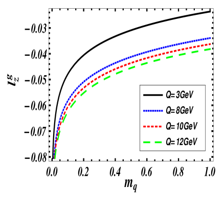
(a)    (b)

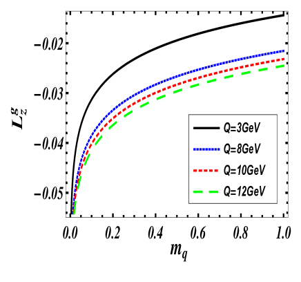
Figure 5: (Color online) Plots of OAM (a) $l^{g}_{z}$ and (b) $L^{g}_{z}$ vs $m_{q}$ (GeV) for different values of $Q$ (GeV).

IV Numerical Results

In Figs. 1 - 4, we have shown the 3D plots for the Wigner distributions of gluon in the impact parameter space ($b_{x}$-$b_{y}$), momentum space ($k_{x}$-$k_{y}$) and also in the mixed space ($k_{y}$-$b_{x}$). Normally the upper limit of the Fourier transform should be infinite. But in our numerical calculation, we chose an upper limit of $\mid\Delta_{\perp}\mid$ which we called $\Delta_{max}$. Plots on the left and right column are for $\Delta_{max}=1$ GeV and $\Delta_{max}=5$ GeV respectively. Dependence of gluon Wigner function on $\Delta_{max}$ is similar as the quark Wigner distributions: the peak of the Wigner distribution increases in magnitude as $\Delta_{max}$ increases. First, second and the third row in all Figs. 1 - 4 correspond to the impact parameter, momentum and mixed space plots respectively. The plots in mixed space have probabilistic interpretation since we have integrated out the variable in the remaining direction i.e. $k_{x}$ and $b_{y}$ and for the impact parameter and momentum space plots these remaining variables are held constant. For all the plots, we have taken mass of target state to be 0.33 GeV. Also we integrated over $x$ and divided by the normalization constant $N$.

In Fig. 1 , we show the 3D plots for the Wigner distribution of unpolarized gluon in an unpolarized target state ($W^{UU}$). In Figs. 1(a) and 1(b) we see the variation of $W^{UU}$ in the position space. The magnitude of $W^{UU}$ is maximum at center ( $b_{x}=b_{y}=0$) and increases with increase in $\Delta_{max}$, which is expected from the analytic expression of $W^{UU}$. In Figs. 1(c) and 1(d) we have plotted $W^{UU}$ in the momentum space for $\vec{b_{\perp}}=b\hat{j}=0.4$. In momentum space too $W^{UU}$ peaks at center ($k_{x}=k_{y}=0$) and its magnitude increases with increasing $\Delta_{max}$. In Figs. 1(e) and 1(f) we have shown the variation of $W^{UU}$ in the mixed space. We observed that $W^{UU}$ is maximum for $k_{y}=0$. As we move away from $k_{y}=0$, it first decreases and then increases. Hence the probability to find a gluon in the target state is maximum near $k_{y}=0$.
It is worth mentioning here that similar plots for the quark Wigner distributions in our1 are rotated through an angle ${\pi\over 4}$ because there we took $\Delta_{\perp}$ to be positive only whereas here we took $\Delta_{\perp}$ to be both positive and negative.

In Fig. 2, we show the 3D plots for the Wigner distribution of unpolarized gluon in longitudinally polarized target state. In Figs. 2(a) and 2(b) we see how $W^{LU}$ varies in position space. We observed dipole structure whose magnitude increases with increase in $\Delta_{max}$. In Figs. 2(c) and 2(d) we have plotted $W^{LU}$ in the momentum space for a fixed $\vec{b_{\perp}}=b\hat{j}=0.4$. Again we observe a dipole structure but the polarity is flipped when compared to the plots in position space. Also, the magnitude of the peak increases with increasing $\Delta_{max}$ which is expected from the analytic expression of $W^{LU}$. In Figs. 2(e) and 2(f) we have shown the variation of $W^{LU}$ in the mixed space. Here we observe quadrupole structure whose magnitude increases with increase in $\Delta_{max}$.

In Fig.  3, we show the 3D plots for the Wigner distribution showing the distortion due to the longitudinal polarization of the gluons. In Figs. 3(a) and 3(b) we show the variation of $W^{UL}$ varies in position space for fixed $\vec{k_{\perp}}=k\hat{j}=0.4$. We observe that the behavior is similar to the case of $W^{LU}$ showing a dipole structure. In Figs. 3(c) and 3(d) we have plotted $W^{UL}$ in the momentum space for $\vec{b_{\perp}}=b\hat{j}=0.4$. In the momentum space we observe a dipole like structure again similar to the case of $W^{LU}$ but here the polarity is not flipped unlike that in $W^{UL}$ when compared to the plots in the position space. In the mixed space we again observe a quadruple structure with increasing magnitude as $\Delta_{max}$ increases.

In Fig.  4, we show the 3D plots for the Wigner distribution showing the distortion due to the correlation between the longitudinal polarization of the target state and the gluons. In Figs. 4(a) and 4(b) we see how $W^{LL}$ varies in position space. In the b-space the behavior is similar to that shown by $W^{UU}$ and the magnitude increases with increasing $\Delta_{max}$ value. In Figs. 4(c) and 4(d) we have plotted $W^{LL}$ in the momentum space for $\vec{b_{\perp}}=b\hat{j}=0.4$. In momentum space, $W^{LL}$ shows a behavior similar to that of $W^{UU}$ and its magnitude increases with increasing $\Delta_{max}$. In the mixed space again the nature is identical to that shown by $W^{UU}$.

In Fig 5, we have plotted the OAM of gluon with respect to mass of the target state for different values of $Q$ where $Q$ and $\mu$ are the upper and lower limits of transverse momentum integration respectively. $\mu$ can be taken to be zero if the quark mass is non-zero. In fact we take taken $\mu$ to be zero. In Figs. 5(a) and 5(b) we show the canonical and the kinetic gluon OAM respectively as a function of the target mass. We observe that the magnitude of both the OAM decreases with increasing mass of target state.

V Conclusion

In this work, we presented a calculation of gluon Wigner distributions for a quark state dressed with a gluon. This can be thought of as a simple composite spin ${1/2}$ system having a gluonic degree of freedom. We showed the various correlations between the gluon spin and the spin of the target. We calculated the gluon kinetic and canonical OAM and also calculated the spin-orbit interaction of the gluons. The kinetic and canonical OAM of the gluons differ in magnitude. In most phenomenological models, there is no gluonic degree of freedom and a study of gluonic contribution to the spin and OAM is not possible in such models. Our simple field theoretical model calculations may be considered as a first step towards understanding the gluon spin and OAM contribution.

VI ACKNOWLEDGMENTS

We would like to thank C. Lorce for helpful discussions. This work is supported by the DST project SR/S2/HEP-029/2010, Govt. of India.