Cusp bifurcation in the eigenvalue spectrum of $\mathcal{PT}$-symmetric Bose-Einstein condensates

Abstract

A Bose-Einstein condensate in a double-well potential features stationary solutions even for attractive contact interaction as long as the particle number and therefore the interaction strength do not exceed a certain limit. Introducing balanced gain and loss into such a system drastically changes the bifurcation scenario at which these states are created. Instead of two tangent bifurcations at which the symmetric and antisymmetric states emerge, one tangent bifurcation between two formerly independent branches arises [D. Haag et al., Phys. Rev. A 89, 023601 (2014)]. We study this transition in detail using a bicomplex formulation of the time-dependent variational principle and find that in fact there are three tangent bifurcations for very small gain-loss contributions which coalesce in a cusp bifurcation.

I Introduction

Bose-Einstein condensates with attractive contact interactions become unstable if the number of particles exceeds a certain limit Ruprecht et al. (1995); Dodd et al. (1996); Houbiers and Stoof (1996). In mean-field approximation where the condensate is described by the Gross-Pitaevskii equation this effect manifests itself in a vanishing ground state. Above this limit the mean interaction caused by the particles is strong enough to constrict and ultimately collapse the condensate. Below this limit the stationary solutions of the Gross-Pitaevskii equation are observable even though for attractive interactions the ground state is not the global minimum of the mean-field energy Sackett et al. (1997).

Characteristic properties of Bose-Einstein condensates with attractive interaction could be used for an atomic soliton laser Ruprecht et al. (1995). However, this requires the realization of a particle flow into and out of the condensate. Modeling such effects in mean-field approximation is done via imaginary potentials, thus rendering the Hamiltonian non-Hermitian Moiseyev (2011); Kagan et al. (1998). Such non-Hermitian systems have been widely studied Kagan et al. (1998); Schlagheck and Paul (2006); Rapedius and Korsch (2009); Rapedius et al. (2010); Abdullaev et al. (2010); Bludov and Konotop (2010); Witthaut et al. (2011) and are supported by comparison with many-particle calculations Rapedius (2013); Dast et al. (2014). Both in- and outcoupling of particles have been experimentally realized Gericke et al. (2008); Robins et al. (2008).

Despite the non-Hermiticity real eigenvalues and thus true stationary states can be found if the Hamiltonian is $\mathcal{PT}$-symmetric Bender and Boettcher (1998); Bender et al. (1999); Bender (2007) or pseudo-Hermitian Mostafazadeh (2002a, b, c). This unique property motivated a variety of theoretical studies Klaiman et al. (2008); Schindler et al. (2011); Bittner et al. (2012); Cartarius et al. (2012); Cartarius and Wunner (2012); Mayteevarunyoo et al. (2013); Graefe et al. (2008a, b); Graefe (2012) and the experimental realization in optical wave-guide systems Klaiman et al. (2008); Rüter et al. (2010); Guo et al. (2009); Peng et al. (2014).

In Haag et al. (2014) we studied the eigenvalue spectrum and dynamical properties of a Bose-Einstein condensate, described by the dimensionless Gross-Pitaevskii equation

$$(-\Delta+V_{\mathrm{ext}}+8\pi Na|\psi|^{2})\psi=\mu\psi,$$ (1)

in a three-dimensional $\mathcal{PT}$-symmetric double-well potential

$$V_{\mathrm{ext}}(\mathbf{x})=\frac{1}{4}[x^{2}+\omega^{2}(y^{2}+z^{2})]+v_{0}\mathrm{e}^{-\sigma x^{2}}+\mathrm{i}\gamma x\mathrm{e}^{-\rho x^{2}},$$ (2)

with $\omega=2$, $v_{0}=4$, $\sigma=0.5$ and $\rho\approx 0.12$. The symmetric real part of the potential is a harmonic trap which is separated into two wells by a Gaussian barrier. The antisymmetric imaginary part of the potential induces particle loss in the left well and particle gain in the right well whose strength is given by the gain-loss parameter $\gamma$.

It was found that four stationary states of the real double-well potential are created in the two lowest-lying tangent bifurcations at strong attractive interaction strengths $Na$. If gain and loss is introduced into the system, instead of two bifurcations there is only one bifurcation between two previously independent states, while the other two states vanish. However, the underlying bifurcation mechanism remained unclear. It is the purpose of this paper to clarify this mechanism and study the bifurcation scenario in detail classifying it as a cusp bifurcation Poston and Stewart (1978).

The number of solutions is not conserved at bifurcations since the Gross-Pitaevskii equation is non-analytic due to its nonlinear part $|\psi|^{2}$. This problem is addressed by applying an analytic continuation, where the complex wave functions are replaced by bicomplex ones. The numerical results are then obtained via the time-dependent variational principle (TDVP).

We start with a short introduction to bicomplex numbers in Sec. II before discussing their application to the Gross-Pitaevskii equation and the TDVP in Sec. III. A detailed analysis of the eigenvalue spectrum and the bifurcation scenario is carried out in Sec. IV. Conclusions are drawn in Sec. V.

II Bicomplex numbers

Consider a usual complex number $z\in\mathbb{C}$, $z=x+\mathrm{i}y$ with $x,y\in\mathbb{R}$ and the imaginary unit $\mathrm{i}^{2}=-1$. A bicomplex number is constructed by replacing the real and imaginary part of $z$ by complex numbers with an additional imaginary unit $\mathrm{j}$ which also fulfills $\mathrm{j}^{2}=-1$,

$$z=x+\mathrm{i}y=(x_{1}+\mathrm{j}x_{\mathrm{j}})+\mathrm{i}(y_{1}+\mathrm{j}y_{\mathrm{j}})\equiv z_{1}+\mathrm{i}z_{\mathrm{i}}+\mathrm{j}z_{\mathrm{j}}+\mathrm{k}z_{\mathrm{k}}.$$ (3)

In the last step $\mathrm{k}=\mathrm{i}\mathrm{j}$ with $\mathrm{k}^{2}=1$ was introduced.

Every bicomplex number can be uniquely written Gervais Lavoie et al. (2010, 2011) as

$$z=z_{+}e_{+}+z_{-}e_{-},$$ (4)

with the components

$$z_{+} =(z_{1}+z_{\mathrm{k}})+\mathrm{i}(z_{\mathrm{i}}-z_{\mathrm{j}}),$$ (5a)

$$z_{-} =(z_{1}-z_{\mathrm{k}})+\mathrm{i}(z_{\mathrm{i}}+z_{\mathrm{j}}),$$ (5b)

and the idempotent basis

$$e_{\pm}=\frac{1\pm\mathrm{k}}{2}.$$ (6)

One can easily confirm that $e_{\pm}$ fulfill the relations

$$e_{+}+e_{-}=1,\quad e_{+}-e_{-}=\mathrm{k},\quad e_{+}e_{-}=0,\quad e_{\pm}^{2}=e_{\pm}.$$ (7)

Note that an equivalent representation exists in which the components $z_{\pm}$ are complex numbers with the imaginary unit $\mathrm{j}$ instead of the imaginary unit $\mathrm{i}$.

The introduction of the idempotent basis significantly simplifies arithmetic operations of bicomplex numbers since for two bicomplex numbers $z,w$ the relation

$$z\circ w=(z_{+}\circ w_{+})e_{+}+(z_{-}\circ w_{-})e_{-}$$ (8)

holds, where $\circ$ represents addition, subtraction, multiplication and division. Thus the bicomplex algebra is effectively reduced to a complex algebra within the coefficients.

III Numerical method

As a next step we apply the analytic continuation to the Gross-Pitaevskii equation (1) by allowing bicomplex values for the wave function $\psi$ and the chemical potential $\mu$. With the notation introduced in Eq. (4) the modulus squared can be written as $|\psi|^{2}=\psi\psi^{*}=\psi_{+}\psi_{-}^{*}e_{+}+\psi_{-}\psi_{+}^{*}e_{-}$. Here $\psi^{*}$ denotes a complex conjugation of $\psi$ with respect to the complex unit $\mathrm{i}$. Since $\mathrm{k}=\mathrm{i}\mathrm{j}$ this complex conjugation changes also the sign of $\mathrm{k}$ and thus transforms $e_{+}$ into $e_{-}$ and vice versa. Due to the properties (7) and (8) the $\pm$ components are independent and the bicomplex Gross-Pitaevskii equation can be split into two coupled complex differential equations, which evidently do not contain a non-analytical term anymore,

$$(-\Delta+V_{\mathrm{ext}}+8\pi Na\psi_{+}\psi_{-}^{*})\psi_{+} =\mu_{+}\psi_{+},$$ (9a)

$$(-\Delta-V_{\mathrm{ext}}+8\pi Na\psi_{-}\psi_{+}^{*})\psi_{-} =\mu_{-}\psi_{-}.$$ (9b)

For complex wave functions the relation $\psi_{+}=\psi_{-}$ holds, as can be seen in Eqs. (5), and the Eqs. (9) are reduced to the Gross-Pitaevskii equation (1). Thus, the coupled Eqs. (9) still support all solutions of the Gross-Pitaevskii equation (1).

To solve the Eqs. (9) the TDVP is generalized for bicomplex differential equations. Our ansatz consists of coupled Gaussian wave packets which yields accurate results even for a small number of wave packets Rau et al. (2010a, b, c). For the double-well potential studied in this work it was shown that two coupled Gaussian wave packets suffice and additional wave packets only lead to small corrections Dast et al. (2013a); Haag et al. (2014). For all calculations the following bicomplex ansatz is used

$$\psi(\mathbf{x},\mathbf{z}(t))=\sum_{n=1}^{2}\exp(-\mathbf{x}^{T}A^{n}\mathbf{x}+\mathbf{b}^{n}\cdot\mathbf{x}+c^{n}),$$ (10)

with the bicomplex three-dimensional diagonal matrix $A^{n}=\operatorname{diag}(A^{n}_{\parallel},A^{n}_{\perp},A^{n}_{\perp})$, the bicomplex three-dimensional vector $\mathbf{b}^{n}=(b^{n},0,0)^{T}$, and the bicomplex number $c^{n}$. The vector $\mathbf{z}(t)$ contains all parameters $A^{n},$ $\mathbf{b}^{n}$, $c^{n}$ of the wave function. The ansatz is chosen such that all solutions are invariant under rotations around the $x$ axis, i.e. we search only for wave functions that possess the symmetry of the potential. The complex $\pm$ components of the wave function can be written as

$$\psi_{\pm}(\mathbf{x},\mathbf{z}_{\pm}(t)) =\sum_{n=1}^{2}\exp(-\mathbf{x}^{T}A_{\pm}^{n}\mathbf{x}+\mathbf{b}_{\pm}^{n}\cdot\mathbf{x}+c_{\pm}^{n})$$

$$\equiv\sum_{n=1}^{2}g_{\pm}^{n}$$ (11)

using Eq. (8) since the exponential function is defined as a power series.

The TDVP makes use of the McLachlan variational principle McLachlan (1964) which demands that the variation of the functional

$$I=\|\mathrm{i}\varphi-\mathcal{H}\psi\|^{2}$$ (12)

with respect to $\varphi$ vanishes, then after the variation $\varphi=\dot{\psi}$ is set. Using the representation with the idempotent basis (4) for $\varphi$, $\psi$ and $\mathcal{H}$ leads to

$$I= \langle{\mathrm{i}\varphi_{-}-\mathcal{H}_{-}\psi_{-}}|{\mathrm{i}\varphi_{+}-\mathcal{H}_{+}\psi_{+}}\rangle e_{+}$$

$$+\langle{\mathrm{i}\varphi_{+}-\mathcal{H}_{+}\psi_{+}}|{\mathrm{i}\varphi_{-}-\mathcal{H}_{-}\psi_{-}}\rangle e_{-}$$

$$\equiv I_{+}e_{+}+I_{-}e_{-}$$ (13)

The two coefficients are complex conjugate, thus, the functional $\tilde{I}=I_{+}=I_{-}^{*}$ already contains the full information. The variation of the functional $\tilde{I}$ reads,

$$\delta\tilde{I} =\langle{\mathrm{i}\delta\varphi_{-}}|{\mathrm{i}\varphi_{+}-\mathcal{H}_{+}\psi_{+}}\rangle+\langle{\mathrm{i}\varphi_{-}-\mathcal{H}_{-}\psi_{-}}|{\mathrm{i}\delta\varphi_{+}}\rangle$$

$$=\langle{\mathrm{i}\partial_{\mathbf{z}_{-}}\psi_{-}}|{\mathrm{i}\dot{\psi}_{+}-\mathcal{H}_{+}\psi_{+}}\rangle\delta\dot{\mathbf{z}}_{-}^{*}$$

$$\quad+\langle{\mathrm{i}\dot{\psi}_{-}-\mathcal{H}_{-}\psi_{-}}|{\mathrm{i}\partial_{\mathbf{z}_{+}}\psi_{+}}\rangle\delta\dot{\mathbf{z}}_{+}$$

$$=0.$$ (14)

Since the variations $\delta\dot{\mathbf{z}}_{+}$ and $\delta\dot{\mathbf{z}}_{-}^{*}$ are independent both coefficients have to vanish, which can be written in the compact form

$$\langle{\mathrm{i}\dot{\psi}_{\mp}-\mathcal{H}_{\mp}\psi_{\mp}}|{\partial_{\mathbf{z}_{\pm}}\psi_{\pm}}\rangle=0.$$ (15)

Using the idempotent basis we can reduce the bicomplex equation to a pair of coupled complex equations.

The next step is to insert the ansatz (11) of the wave function into Eq. (15). The calculations are in full analogy with the TDVP for complex Gaussian wave packets Eichler et al. (2012) and therefore we only list the results.

The equations of motion for the parameters of the Gaussian wave packets read

$$\mathrm{i}\dot{A}_{\pm}^{n} =4(A_{\pm}^{n})^{2}-V_{2\pm}^{n},$$ (16a)

$$\mathrm{i}\dot{\mathbf{b}}_{\pm}^{n} =4A_{\pm}^{n}\mathbf{b}_{\pm}^{n}+\mathbf{v}_{1\pm}^{n},$$ (16b)

$$\mathrm{i}\dot{c}_{\pm}^{n} =2\operatorname{tr}{A}_{\pm}^{n}-\mathbf{b}_{\pm}^{n}\cdot\mathbf{b}_{\pm}^{n}+v_{0\pm}^{n}.$$ (16c)

The coefficients of the effective potential $V_{2\pm}^{n}$, $\mathbf{v}_{1\pm}^{n}$ and $v_{0\pm}$ are obtained by numerically solving

$$\sum_{n=1}^{N}\langle{x_{\alpha}^{k}x_{\beta}^{l}g_{\mp}^{m}}|{(\mathbf{x}^{T}V_{2\pm}^{n}\mathbf{x}+\mathbf{v}_{1\pm}^{n}\cdot\mathbf{x}+v_{0\pm}^{n})g_{\pm}^{n}}\rangle$$

$$=\sum_{n=1}^{N}\langle{x_{\alpha}^{k}x_{\beta}^{l}g_{\mp}^{m}}|{(V_{\mathrm{ext}}+8\pi Na\psi_{\mp}^{*}\psi_{\pm})g_{\pm}^{n}}\rangle,$$ (17)

with $\alpha,\beta=1,\dots,d$; $m=1,\dots,N$ and $k+l=0,1,2$, where $d$ is the dimension and $N$ the number of coupled Gaussians. For the ansatz (11) used in this work we have $d=3$ and $N=2$.

Stationary solutions are obtained by varying the parameters $A_{\pm}^{n}$, $\mathbf{b}_{\pm}^{n}$, $(c_{\pm}^{n}-c_{\pm}^{N})$, such that they fulfill the equations $\dot{A}_{\pm}^{n}=0$, $\dot{\mathbf{b}}_{\pm}^{n}=0$, $(\dot{c}_{\pm}^{n}-\dot{c}_{\pm}^{N})=0$ for $n=1,\dots,N$. Note that the differences $(c_{\pm}^{n}-c_{\pm}^{N})$ are used since not all parameters $c_{\pm}^{n}$ are free due to the norm constraint and the choice of a global phase. Standard numerical methods for complex numbers can be used to achieve this since all parameters in Eqs. (16) and (17) are complex. This again shows the benefit of the idempotent basis.

IV Results

Before discussing the analytic continuation the real spectrum is investigated. In Haag et al. (2014) the real eigenvalue spectrum of this system has already been studied, however, the bifurcation scenario at strong attractive interactions, on which we concentrate in this paper, was only discussed briefly. In particular the bifurcation scenario was only shown for the gain-loss parameters $\gamma=0$ and $\gamma=0.001$, which, as we will see, does not suffice to understand the bifurcation process in detail.

Figure 1

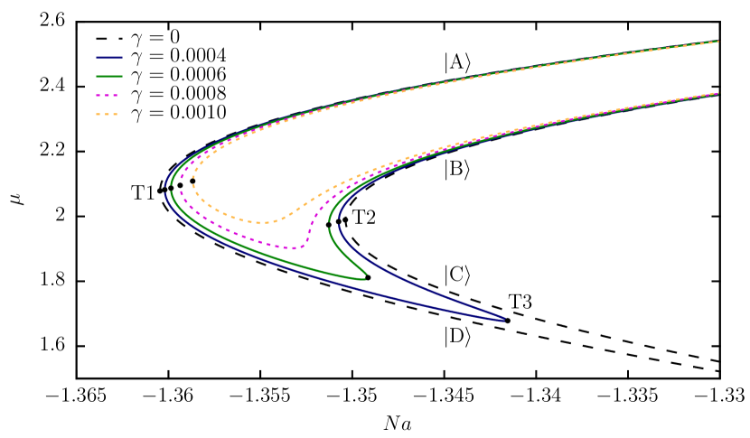
Figure 1: (Color online) The bifurcation scenario of the $\mathcal{PT}$-symmetric stationary states of the three-dimensional double-well potential at strong attractive interactions. The chemical potential of the stationary solutions is shown as a function of the interaction strength $Na$ for different values of the gain-loss parameter $\gamma$. For $\gamma=0$ (black dashed line) two tangent bifurcations T1 and T2 are present. The states $|{\mathrm{A}}\rangle$ and $|{\mathrm{D}}\rangle$ emerge from the bifurcation T1 whereas T2 gives birth to the states $|{\mathrm{B}}\rangle$ and $|{\mathrm{C}}\rangle$. For small values of $\gamma$ (solid lines) a third bifurcation T3 appears at which the two states $|{\mathrm{B}}\rangle$ and $|{\mathrm{C}}\rangle$ bifurcate which connects the so far independent branches of the states $|{\mathrm{C}}\rangle$ and $|{\mathrm{D}}\rangle$. For higher values of $\gamma$ (dotted lines) the bifurcations T2 and T3 vanish, as does the intermediate state $|{\mathrm{C}}\rangle$, thus, the branches of the states $|{\mathrm{B}}\rangle$ and $|{\mathrm{D}}\rangle$ merge.

shows the relevant part of the eigenvalue spectrum as a function of the nonlinearity parameter $Na$ for different gain-loss parameters $\gamma$. All states are $\mathcal{PT}$-symmetric, therefore, their chemical potentials $\mu$ are real. For a vanishing gain-loss contribution, $\gamma=0$, the two states $|{\mathrm{A}}\rangle$ and $|{\mathrm{B}}\rangle$, which originate from the ground and excited state of the double-well potential, emerge from independent tangent bifurcations T1 and T2. The bifurcation T1 gives birth to the states $|{\mathrm{A}}\rangle$ and $|{\mathrm{D}}\rangle$ whereas the states $|{\mathrm{B}}\rangle$ and $|{\mathrm{C}}\rangle$ emerge from the bifurcation T2. At $\gamma=0.001$ the situation has changed fundamentally. The two branches $|{\mathrm{A}}\rangle$ and $|{\mathrm{B}}\rangle$ are no longer independent but emerge from the same bifurcation T1. In addition the branches $|{\mathrm{C}}\rangle$ and $|{\mathrm{D}}\rangle$ have vanished.

This behavior can be understood by studying the system for very small parameters $\gamma$. For $\gamma=0.0004$ both tangent bifurcations T1 and T2, and thus, also the branches $|{\mathrm{C}}\rangle$ and $|{\mathrm{D}}\rangle$ are still present. However, the two pairs emerging from T1 and T2 are now connected by a new tangent bifurcation T3 at which the lower lying states vanish. If the gain-loss parameter is slightly increased the bifurcation T3 is shifted to lower values of $Na$ and approaches T2 ($\gamma=0.0006$). For $\gamma=0.0008$ both bifurcations T2 and T3 have united and vanished.

To discuss the propagation of the two tangent bifurcations in the parameter space in more detail, a phase diagram is shown in Fig. 2.

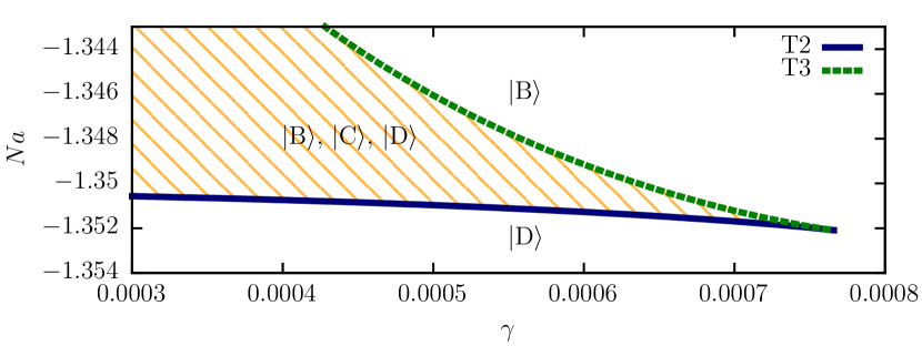
Figure 2: (Color online) Trajectories of the two tangent bifurcations T2 and T3 in the $\gamma$-$Na$-parameter space. In the shaded area all three states involved in the two bifurcations are present while in the other areas only one of these states exists. For increasing values of the gain-loss parameter $\gamma$, the bifurcation T2 is strongly shifted to lower nonlinearity parameters $Na$. At $\gamma_{\mathrm{c}}\approx 0.000766$ the two bifurcations coincide and the state $|{\mathrm{C}}\rangle$ vanishes while the states $|{\mathrm{B}}\rangle$ and $|{\mathrm{D}}\rangle$ merge.

The two bifurcations coalesce and vanish at critical values of the gain-loss parameter $\gamma_{\mathrm{c}}\approx 0.000766$ and interaction strength $(Na)_{\mathrm{c}}\approx-1.352$. Their trajectories have the characteristic form of a cusp in the phase diagram. In the area enclosed by the two trajectories all three states $|{\mathrm{B}}\rangle$, $|{\mathrm{C}}\rangle$, and $|{\mathrm{D}}\rangle$ involved in this bifurcation scenario are present. Outside of this area only one state remains. Below the trajectory of T2 only the state $|{\mathrm{D}}\rangle$ exists and above the trajectory of T3 only the state $|{\mathrm{B}}\rangle$. Since the areas below T2 and above T3 are connected for $\gamma>\gamma_{\mathrm{c}}$, the states $|{\mathrm{B}}\rangle$ and $|{\mathrm{D}}\rangle$ can continuously be transferred into each other by following a path in the parameter space around the cusp.

We have seen that the transition from the $\gamma=0$ case, where the states $|{\mathrm{A}}\rangle$ and $|{\mathrm{B}}\rangle$ are completely independent, to the $\gamma=0.001$ case, where both states emerge from a common bifurcation, occurs in two steps. The first step is the formation of a new tangent bifurcation T3 between the states $|{\mathrm{C}}\rangle$ and $|{\mathrm{D}}\rangle$ and the second step is the coalescence of the two bifurcations. In the following we will show that introducing bicomplex numbers to analytically continue the Gross-Pitaevskii equation allows a more detailed discussion of these two steps.

Bifurcation scenarios are classified by comparison with normal forms Poston and Stewart (1978). The eigenvalue spectrum shows three tangent bifurcations which are described by the normal form $\dot{x}=x^{2}-\sigma$. The stationary solutions, $\dot{x}=0$, are obviously $x=\pm\sqrt{\sigma}$. Two real solutions exist for $\sigma>0$, they coalesce at $\sigma=0$, where two complex conjugate solutions ($\sigma<0$) emerge. Thus, the total number of solutions stays constant if we allow $x$ to be complex. Due to the non-analytic modulus squared in the Gross-Pitaevskii equation this conservation of solutions is not guaranteed although the wave functions can be complex.

In analogy with the transition from real to complex numbers in the normal form of the tangent bifurcation, we expect a transition from complex to bicomplex numbers in the eigenvalue spectrum of the Gross-Pitaevskii equation. By introducing bicomplex numbers the Gross-Pitaevskii equation is analytically continued and the two coupled analytic Eqs. (9) are obtained.

The bicomplex chemical potential $\mu$ of the stationary solutions is shown in Fig. 3.

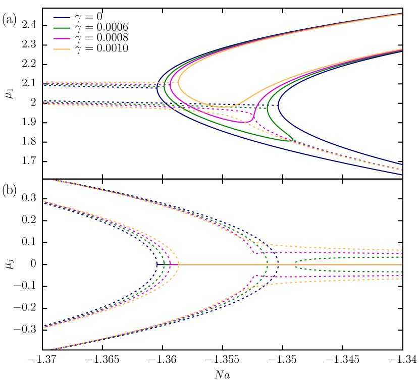
Figure 3: (Color online) Bicomplex bifurcation scenario showing the $\mu_{1}$ and $\mu_{\mathrm{j}}$ component of the chemical potential as a function of the nonlinearity parameter $Na$ for different values of the gain-loss parameter $\gamma$. The $\mathrm{i}$ and $\mathrm{k}$ components vanish for all states discussed, thus $\mu^{*}=\mu$ holds and all states are $\mathcal{PT}$ symmetric. The states with purely real chemical potential, i.e. $\mu_{\mathrm{j}}=0$, are still present (solid lines). In addition a pair of bicomplex states with $\mu=\mu_{1}\pm\mathrm{j}\mu_{\mathrm{j}}$ emerges at the tangent bifurcations T1, T2, and T3 (dotted lines). For $\gamma>\gamma_{\mathrm{c}}$, the bifurcations T2 and T3 have vanished leading to a bicomplex branch that is completely independent from the remaining scenario. Independent of the parameters $\gamma$ and $Na$ there are four stationary solutions.

For the discussion of the results we again use the components of bicomplex numbers as introduced in Eq. (3) instead of the representation in the idempotent basis since this renders the interpretation of the results much clearer. The first thing to note is that all states have vanishing $\mu_{\mathrm{i}}$ and $\mu_{\mathrm{k}}$ components. Therefore $\mu^{*}=\mu$ holds and all states considered are $\mathcal{PT}$ symmetric. All states discussed so far are still present in the spectrum and only have a non-vanishing $\mu_{1}$ component (solid lines). However, additional states with $\mu_{\mathrm{j}}\neq 0$ are found (dotted lines). Since the potential in the Gross-Pitaevskii equation is symmetric under a complex conjugation with respect to $\mathrm{j}$, these states have to appear in pairs $\mu=\mu_{1}+\mathrm{j}\mu_{\mathrm{j}}$ and $\mu=\mu_{1}-\mathrm{j}\mu_{\mathrm{j}}$ Dast et al. (2013b).

First we discuss the case $\gamma<\gamma_{\mathrm{c}}$ where all three tangent bifurcations are present. At the bifurcation T1 the states $|{\mathrm{A}}\rangle$ and $|{\mathrm{D}}\rangle$ coalesce and vanish. On the other side of the bifurcation two bicomplex states emerge whose chemical potentials are complex conjugate with respect to $\mathrm{j}$. Also at the bifurcations T2 and T3 two states of the real spectrum vanish and on the other side of the bifurcations two bicomplex states emerge. For $\gamma>\gamma_{\mathrm{c}}$ the situation at the bifurcation T1 has not changed, however, the bifurcations T2 and T3 have vanished and the states $|{\mathrm{B}}\rangle$ and $|{\mathrm{D}}\rangle$ have merged. The bicomplex states that emerged from T2 and T3 have also merged and form independent branches that do not bifurcate with any real branch.

At the tangent bifurcations two eigenvectors and the corresponding eigenvalues become equal qualifying them as exceptional points of second order Heiss (2012); Demange and Graefe (2012). The bicomplex analysis reveals that at the cusp point, where the bifurcations T2 and T3 merge, a total of three states, one with real eigenvalue and two with bicomplex eigenvalues, coalesce. This is characteristic of an exceptional point of third order which has already been observed in spectra with similar cusp-like behavior Gutöhrlein et al. (2013); Am-Shallem et al. (2014).

The coalescence of two tangent bifurcations is the characteristic property of a cusp bifurcation Poston and Stewart (1978) which is described by the normal form

$$\dot{x}=x^{3}+\rho x-\sigma,$$ (18)

whose stationary solutions $\dot{x}=0$ are found by Cardano’s method. The spectrum of the normal form has two tangent bifurcations which vanish at the critical values $\rho_{\mathrm{c}}=\sigma_{\mathrm{c}}=0$. In Fig. 4

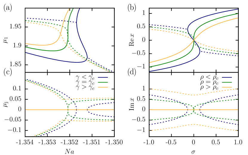
Figure 4: (Color online) Comparison of the cusp bifurcation occurring in the eigenvalue spectrum (left panels) and in the normal form (18) (right panels). For parameter values smaller than the critical value ($\gamma<\gamma_{\mathrm{c}}$, $\rho<\rho_{\mathrm{c}}$) the tangent bifurcations T2 and T3 are separated. They coalesce at the critical parameter value ($\gamma=\gamma_{\mathrm{c}}$, $\rho=\rho_{\mathrm{c}}$) and vanish for $\gamma>\gamma_{\mathrm{c}}$, $\rho>\rho_{\mathrm{c}}$. Real branches are drawn as solid lines and (bi)complex branches as dotted lines.

the normal form is compared with the eigenvalue spectrum of the double-well potential. The parameters $\rho$ and $\sigma$ play the role of the gain-loss parameter $\gamma$ and the nonlinearity parameter $Na$, respectively. At the tangent bifurcations in the eigenvalue spectrum real values of the chemical potential $\mu$ turn into bicomplex values with a $\mathrm{j}$ component, $\mu=\mu_{1}+\mathrm{j}\mu_{\mathrm{j}}$, whereas in the spectrum of the normal form real values become ordinary complex numbers. Thus, we have to compare $\mu_{1}$ with $\operatorname{Re}x$ and $\mu_{\mathrm{j}}$ with $\operatorname{Im}x$. Again the real branches are drawn as solid lines whereas the complex and bicomplex branches are drawn as dotted lines.

In the regime $\gamma<\gamma_{\mathrm{c}}$, $\rho<\rho_{\mathrm{c}}$ the two tangent bifurcations are still separated, at $\gamma=\gamma_{\mathrm{c}}$, $\rho=\rho_{\mathrm{c}}$ the tangent bifurcations coalesce and finally for $\gamma>\gamma_{\mathrm{c}}$, $\rho>\rho_{\mathrm{c}}$ the bifurcations have vanished. The normal form captures the qualitative behavior of the bifurcation scenario found in the eigenvalue spectrum, thus justifying its classification as a cusp bifurcation.

V Conclusion and outlook

This answers the question raised in Haag et al. (2014) regarding the bifurcation scenario at strong attractive interactions and, thus, completes the discussion of the eigenvalue spectrum of the three-dimensional $\mathcal{PT}$-symmetric double-well potential. Formulating the TDVP with bicomplex numbers in the idempotent basis has proved to be useful to analytically continue the non-analytic Gross-Pitaevskii equation and analyze the bifurcation scenarios in the eigenvalue spectrum. Using this formalism will help tackling problems with more complicated $\mathcal{PT}$-symmetric potentials and additional interactions such as the dipolar interaction which might show an even richer variety of bifurcation scenarios.

References

- Ruprecht et al. (1995) P. A. Ruprecht, M. J. Holland, K. Burnett, and M. Edwards, Phys. Rev. A 51, 4704 (1995).
- Dodd et al. (1996) R. J. Dodd, M. Edwards, C. J. Williams, C. W. Clark, M. J. Holland, P. A. Ruprecht, and K. Burnett, Phys. Rev. A 54, 661 (1996).
- Houbiers and Stoof (1996) M. Houbiers and H. T. C. Stoof, Phys. Rev. A 54, 5055 (1996).
- Sackett et al. (1997) C. Sackett, C. Bradley, M. Welling, and R. Hulet, Appl. Phys. B 65, 433 (1997).
- Moiseyev (2011) N. Moiseyev, Non-Hermitian Quantum Mechanics (Cambridge University Press, Cambridge, 2011).
- Kagan et al. (1998) Y. Kagan, A. E. Muryshev, and G. V. Shlyapnikov, Phys. Rev. Lett. 81, 933 (1998).
- Schlagheck and Paul (2006) P. Schlagheck and T. Paul, Phys. Rev. A 73, 023619 (2006).
- Rapedius and Korsch (2009) K. Rapedius and H. J. Korsch, J. Phys. B 42, 044005 (2009).
- Rapedius et al. (2010) K. Rapedius, C. Elsen, D. Witthaut, S. Wimberger, and H. J. Korsch, Phys. Rev. A 82, 063601 (2010).
- Abdullaev et al. (2010) F. K. Abdullaev, V. V. Konotop, M. Salerno, and A. V. Yulin, Phys. Rev. E 82, 056606 (2010).
- Bludov and Konotop (2010) Y. V. Bludov and V. V. Konotop, Phys. Rev. A 81, 013625 (2010).
- Witthaut et al. (2011) D. Witthaut, F. Trimborn, H. Hennig, G. Kordas, T. Geisel, and S. Wimberger, Phys. Rev. A 83, 063608 (2011).
- Rapedius (2013) K. Rapedius, J. Phys. B 46, 125301 (2013).
- Dast et al. (2014) D. Dast, D. Haag, H. Cartarius, and G. Wunner, Phys. Rev. A 90, 052120 (2014).
- Gericke et al. (2008) T. Gericke, P. Wurtz, D. Reitz, T. Langen, and H. Ott, Nat. Phys. 4, 949 (2008).
- Robins et al. (2008) N. P. Robins, C. Figl, M. Jeppesen, G. R. Dennis, and J. D. Close, Nat. Phys. 4, 731 (2008).
- Bender and Boettcher (1998) C. M. Bender and S. Boettcher, Phys. Rev. Lett. 80, 5243 (1998).
- Bender et al. (1999) C. M. Bender, S. Boettcher, and P. N. Meisinger, J. Math. Phys. 40, 2201 (1999).
- Bender (2007) C. M. Bender, Rep. Prog. Phys. 70, 947 (2007).
- Mostafazadeh (2002a) A. Mostafazadeh, J. Math. Phys. 43, 205 (2002a).
- Mostafazadeh (2002b) A. Mostafazadeh, J. Math. Phys. 43, 2814 (2002b).
- Mostafazadeh (2002c) A. Mostafazadeh, J. Math. Phys. 43, 3944 (2002c).
- Klaiman et al. (2008) S. Klaiman, U. Günther, and N. Moiseyev, Phys. Rev. Lett. 101, 080402 (2008).
- Schindler et al. (2011) J. Schindler, A. Li, M. C. Zheng, F. M. Ellis, and T. Kottos, Phys. Rev. A 84, 040101 (2011).
- Bittner et al. (2012) S. Bittner, B. Dietz, U. Günther, H. L. Harney, M. Miski-Oglu, A. Richter, and F. Schäfer, Phys. Rev. Lett. 108, 024101 (2012).
- Cartarius et al. (2012) H. Cartarius, D. Haag, D. Dast, and G. Wunner, J. Phys. A 45, 444008 (2012).
- Cartarius and Wunner (2012) H. Cartarius and G. Wunner, Phys. Rev. A 86, 013612 (2012).
- Mayteevarunyoo et al. (2013) T. Mayteevarunyoo, B. A. Malomed, and A. Reoksabutr, Phys. Rev. E 88, 022919 (2013).
- Graefe et al. (2008a) E. M. Graefe, H. J. Korsch, and A. E. Niederle, Phys. Rev. Lett. 101, 150408 (2008a).
- Graefe et al. (2008b) E. M. Graefe, U. Günther, H. J. Korsch, and A. E. Niederle, J. Phys. A 41, 255206 (2008b).
- Graefe (2012) E.-M. Graefe, J. Phys. A 45, 444015 (2012).
- Rüter et al. (2010) C. E. Rüter, K. G. Makris, R. El-Ganainy, D. N. Christodoulides, M. Segev, and D. Kip, Nat. Phys. 6, 192 (2010).
- Guo et al. (2009) A. Guo, G. J. Salamo, D. Duchesne, R. Morandotti, M. Volatier-Ravat, V. Aimez, G. A. Siviloglou, and D. N. Christodoulides, Phys. Rev. Lett. 103, 093902 (2009).
- Peng et al. (2014) B. Peng, Ş. K. Özdemir, F. Lei, F. Monifi, M. Gianfreda, G. L. Long, S. Fan, F. Nori, C. M. Bender, and L. Yang, Nat. Phys. 10, 394 (2014).
- Haag et al. (2014) D. Haag, D. Dast, A. Löhle, H. Cartarius, J. Main, and G. Wunner, Phys. Rev. A 89, 023601 (2014).
- Poston and Stewart (1978) T. Poston and I. Stewart, Catastrophe theory and its applications (Pitman, London, 1978).
- Gervais Lavoie et al. (2010) R. Gervais Lavoie, L. Marchildon, and D. Rochon, Ann. Funct. Anal. 1, 75 (2010).
- Gervais Lavoie et al. (2011) R. Gervais Lavoie, L. Marchildon, and D. Rochon, Adv. Appl. Clifford Algebras 21, 561 (2011).
- Rau et al. (2010a) S. Rau, J. Main, and G. Wunner, Phys. Rev. A 82, 023610 (2010a).
- Rau et al. (2010b) S. Rau, J. Main, H. Cartarius, P. Köberle, and G. Wunner, Phys. Rev. A 82, 023611 (2010b).
- Rau et al. (2010c) S. Rau, J. Main, P. Köberle, and G. Wunner, Phys. Rev. A 81, 031605(R) (2010c).
- Dast et al. (2013a) D. Dast, D. Haag, H. Cartarius, G. Wunner, R. Eichler, and J. Main, Fortschr. Physik 61, 124 (2013a).
- McLachlan (1964) A. D. McLachlan, Mol. Phys. 8, 39 (1964).
- Eichler et al. (2012) R. Eichler, D. Zajec, P. Köberle, J. Main, and G. Wunner, Phys. Rev. A 86, 053611 (2012).
- Dast et al. (2013b) D. Dast, D. Haag, H. Cartarius, J. Main, and G. Wunner, J. Phys. A 46, 375301 (2013b).
- Heiss (2012) W. D. Heiss, J. Phys. A 45, 444016 (2012).
- Demange and Graefe (2012) G. Demange and E. M. Graefe, J. Phys. A 45, 025303 (2012).
- Gutöhrlein et al. (2013) R. Gutöhrlein, J. Main, H. Cartarius, and G. Wunner, J. Phys. A 46, 305001 (2013).
- Am-Shallem et al. (2014) M. Am-Shallem, R. Kosloff, and N. Moiseyev, “Exceptional points for parameter estimation in open quantum systems: Analysis of the Bloch equations,” (2014), arXiv:1411.6364 [quant-ph] .