Photophysics of single nitrogen-vacancy centers in diamond nanocrystals

Résumé

A study of the photophysical properties of nitrogen-vacancy (NV) color centers in diamond nanocrystals of size of 50 nm or below is carried out by means of second-order time-intensity photon correlation and cross-correlation measurements as a function of the excitation power for both pure charge states, neutral and negatively charged, as well as for the photochromic state, where the center switches between both states at any power. A dedicated three-level model implying a shelving level is developed to extract the relevant photophysical parameters coupling all three levels. Our analysis confirms the very existence of the shelving level for the neutral NV center. It is found that it plays a negligible role on the photophysics of this center, whereas it is responsible for an increasing photon bunching behavior of the negative NV center with increasing power. From the photophysical parameters, we infer a quantum efficiency for both centers, showing that it remains close to unity for the neutral center over the entire power range, whereas it drops with increasing power from near unity to approximately 0.5 for the negative center. The photophysics of the photochromic center reveals a rich phenomenology that is to a large extent dominated by that of the negative state, in agreement with the excess charge release of the negative center being much slower than the photon emission process.

I Introduction

With the development of photonic quantum cryptography and quantum information processes, there is need for reliable and easy-to-use single photon sources. Such sources have been developed in recent years singlephoton , like single molecules, colloidal or epitaxial semiconductor quantum dots, and color-centers in diamond. Gruber97 ; Prawer ; Si-N Here, we are interested in the latter, namely the NV center, formed by a substitutional nitrogen atom adjacent to a vacancy in the diamond lattice. NV centers have found numerous applications recently thanks to their unique physical properties such as excellent photostability Gruber97 ; Brouri00 ; Sonnefraud08 ; Bradac2010 and long spin coherence times Balasubramanian09 as well as to improved control over both their production Rondin10 and physical initialization protocols. Siyushev13 NV centers can be made available both in ultra-pure bulk diamond Balasubramanian09 and ultra-small crystals. Smith08 Applications range from high-sensitivity high-resolution magnetometry Degen08 ; Maze08 ; Balasubramanian08 ; Maletinsky12 ; Rondin12 ; Rondin14 ; Grinolds13 , to fluorescence probing of biological processes  Faklaris09 ; McGuinness11 , solid-state quantum information processing Schuster10 ; Kubo10 , spin optomechanics Arcizet11 ; Hong12 , quantum optics Beveratos01 ; Kurtsiefer00 ; Sipahigil12 , nanophotonics Schietinger09 ; Cuche09 ; Beams13 ; Schell , and quantum plasmonics. Kolesov09 ; Cuche10 ; Mollet12
NV centers can take two different charge states with different spectral properties: the neutral center NV⁰, which has a zero-phonon line (ZPL) around 575 nm (2.16 eV), and the negatively charged center NV^-, which has a ZPL around 637 nm (1.95 eV). Dumeige04 In addition to ZPLs, the fluorescence spectra of both centers exhibit a broad and intense vibronic band at lower energy. A single NV center, as a single-photon emitter, is characterized by a second-order time-intensity correlation function that exhibits a photon antibunching dip at zero delay. In a first approach, the photophysics of NV centers can be modeled by a two-level system with two photophysical parameters, the excitation rate, and the spontaneous emission rate. However, with increasing excitation power, the NV center, more particularly in the negative state NV^-, can experience distinctive photon bunching at finite coincidence time, in addition to the expected antibunching at zero delay. This can be accounted for within a three-level system with additional photophysical parameters to describe photon decays to, or from, the additional shelving level.
The aim of this paper is to give a detailed description of the intrinsic photophysics of single NV centers of both charge states in surface-purified Rondin10 nanodiamonds (NDs) of size around 50 nm, or below, as a function of the illumination power from a CW laser. Understanding the intrinsic photophysics of NV centers is required before implementing small fluorescent NDs in a complex electromagnetic environment, such as practical single-photon devices, which will modify the photophysics. Schietinger09 It is also useful to the applications mentioned above as most of them exploit the single-photon emitter nature of isolated NVs.
The statistics of both NV charge states has been studied previously in ND samples similar to those studied here and it was found to be size dependent, with a larger occurrence (> 80%) of the NV^- center over the entire size range from 20 to 80 nm. Rondin10 In the present study, we further observed that most of the single NV centers being detected as neutral from their fluorescence spectrum at low illumination power (<0.5 mW) progressively gain with increasing power a photochromic character in that they also exhibit the NV^- ZPL in addition to the NV⁰ ZPL. Only a few of NV⁰s remain purely neutral over the entire power range, which we call pure NV⁰ behavior. On the other hand, NV centers detected as negatively charged at low power remain so with increasing power, which we call pure NV^- behavior. We first focus our attention on such pure NV⁰ or NV^- centers. In addition to such behaviors, we found that some rare NVs can see their charge switching between neutral and negative Gaebel06 already at the lowest excitation power. We also describe the photophysics of such a photochromic NV over the same power range as the non-photochromic centers and show how both photophysics can be linked. This allows us to find valuable information on the dynamics of photochromism.
The paper is organized as follows. The experimental methods are described in Section II. The three-level model used to interpret the experiment is developed in detail in Section III. Section IV focuses on the experimental results and on the extraction of the various photophysical parameters as a function of the excitation power for a NV⁰ and a NV^- center. Section V describes the photophysics of photochromism in a single NV. A summary is given in Section VI.

II Experimental methods

Preparation of the ND sample was achieved following a procedure reported previously. Dantelle10 ; Rondin10 Commercial HPHT diamond nanocrystals are first irradiated using high-energy electrons, then annealed at 800 °C in vacuum to produce the fluorescent NV centers, and finally annealed in air at 550 °C to remove surface graphitic compounds. Colloidal dispersion in water and further sonication allow us to obtain a uniform solution of NDs. We consider here NDs with a typical size of 25 nm or 50 nm deposited on a fused silica substrate to minimize spurious fluorescence. Cuche09 Single NV centers were optically addressed using standard confocal microscopy at room temperature. Cuche09 A CW laser light (wavelength $\lambda_{exc}$ = 515 nm) falling within the absorption band of the NVs is used to excite the NV fluorescence. Excitation light was focused onto the sample using an oil immersion microscope objective with numerical aperture NA= 1.4. The NV fluorescence is collected through the same objective and is filtered from the remaining excitation, i.e., with wavelength below 532 nm, by a dichroic mirror and a high-pass filter. The collected fluorescence is subsequently sent either to a Hanbury-Brown and Twiss (HBT) intensity correlator (see below) or to a spectrometer. An example of fluorescence spectrum is shown in Fig. 1(b) for the NV^- case. The ZPL corresponds to the resonant decay (Fig. 1(a)) at $\lambda=637$ nm while the wide fluorescence side-band is the phonon replica.

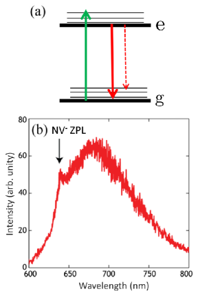
Figure 1: (Color online) (a) Schematic of the two-level system explaining the emission spectrum of the NV center. g : ground state, e : excited state. The several thinner horizontal lines represent the coupling with the phonon bath in the diamond matrix. The green arrow represents the excitation and the red ones the optical decay at resonance (full arrow) and out of resonance (dotted arrow) (b) Typical emission spectrum of an NV^- center in a 25 nm ND.

The second-order time-intensity correlation function contains the information on the classical versus quantum nature of light. It reads in the stationary regime

$$g^{(2)}(\tau)=P_{2}(t+\tau|t)/P_{1}(t)$$ (1)

where $P_{2}(t+\tau|t)=P_{2}(\tau|0)$ is the conditional probability to detect a photon at time $t+\tau$ knowing that another photon has been recorded at time $t$. This probability is normalized by the constant single photon detection rate $P_{1}(t)=P_{1}(0)$. For a classical source of light $g^{(2)}(\tau)\geq 1$, whereas the observation of an anti-bunching $g^{(2)}(\tau)\leq 1$ is a clear signature of the quantum nature of light. Loudon ; Mandel95 ; Kimble In particular, at zero delay $g^{(2)}(0)=0$ for a single photon emitter Kimble , which means that the probability to detect simultaneously two photons vanishes.
In practice, an HBT correlator (Fig. 2(a)) Brouri00 ; Sonnefraud08 is used to measure $g^{(2)}$. Here, the fluorescence of the NV center is sent on a beam splitter, which separates the signal in two equal parts sent to two avalanche photo-diodes (APDs) named APD1 and APD2. The APDs are connected to a time-correlated single-photon counting module to build histograms of delays between photon events detected by the upper «  Start   » APD1 and the lower «  Stop   » APD2. In order to avoid unwanted optical crosstalk between the APDs, a glass filter acting as a short-pass filter at 750 nm and a diaphragm are added in both branches. Kurtsiefer01 In the standard configuration, no bandpass filter is added to the setup, in contrast with the configurations used to study photochromism (Section V), so that it can be used for both charge states of the NV (provided that the NVs do not experience charge conversion, which is the case for the selected NVs in the present work).

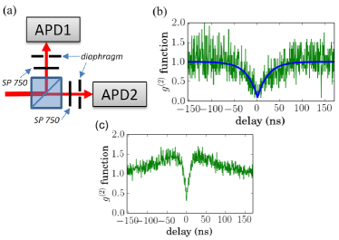
Figure 2: (Color online) (a) Schematic of the HBT correlator (b) Time-intensity second-order correlation function $g^{(2)}(\tau)$ of a NV⁰ center excited at 200 $\mu$ W and presenting an antibunching at zero delay, (c) Time-intensity second-order correlation function $g^{(2)}(\tau)$ of a NV^- center excited at 5 mW and presenting a bunching at finite delay together with the antibunching at zero delay. SP 750 : short-pass filter at 750 nm

III Three-level system: theoretical model

Fig. 2(b) shows a typical $g^{(2)}$ function measured for a single NV at low excitation power. The experimental data are compared with an equation stemming from a two-level model Brouri00 ; Cuche09 :

$$g^{(2)}(\tau)=1-e^{-(r+\gamma)\tau}\,,$$ (2)

where $r$ and $\gamma$ are the excitation and spontaneous emission rates, respectively. Within this model $g^{(2)}(\tau)<1$, which means that the emitted light is non-classical at any delay $\tau$. However, at higher excitation rate this simple model (Eq. 2) generally fails. This is particularly true for NV^- centers. In this case, as shown in Fig. 2(c), the $g^{(2)}$ function includes a bunching $g^{(2)}(\tau)>1$ feature at finite delays, superimposed to the antibunching curve. This kind of correlation profile, which contradicts Eq. 2, calls for a third level that traps the electron, preventing subsequent emission of a photon for a certain time. Doherty1 ; Doherty2 ; Maze ; Gali ; Vincent ; Kehayias ; Gali09 ; Felton08 Therefore, for these delays, the correlation function is higher than one. Though well known for the NV^- center, the existence of a shelving level is less documented for its neutral counterpart but has been invoked theoretically Gali09 as well as in electron-paramagnetic resonance. Felton08 From now on, we will describe phenomenologically the color center dynamics by a three-level model and deduce the intrinsic photo-physical parameters of pure NV^- and NV⁰ centers (Section IV) and of a photochromic center (section V). These NV centers have been selected from their fluorescence spectra.

III.1 Correlation function of a three-level system

In order to give a quantitative description of the three-level model we first review briefly the interpretation of the $g^{(2)}$ function using Einstein’s rate equations. Starting from Glauber quantum measurement theory Glauber we have

$$g^{(2)}(\tau)=\frac{\langle:I(t+\tau)I(t):\rangle}{(\langle I(t)\rangle)^{2}},$$ (3)

where $I(t)$ is the quantum operator equivalent to the electromagnetic energy flow absorbed by a detector at time $t$ and $::$ represents normal ordering. Loudon ; Mandel95 Introducing the creation and annihilation photon operators $a^{\dagger}(t)$ and $a(t)$ in the Heisenberg representation, we obtain:

$$g^{(2)}(\tau)=\dfrac{\langle a^{\dagger}(t)a^{\dagger}(t+\tau)a(t+\tau)a(t)\rangle}{\lvert\langle a^{\dagger}(t)a(t)\rangle\lvert^{2}}.$$ (4)

For a two-level system with ground state $g$ and excited state $e$, the creation operator $a^{\dagger}(t)$ at time $t$ is to a good approximation proportional to the rising transition operator $\lvert e,t\rangle\langle g,t\lvert$ Milonni , we deduce

$$g^{(2)}(\tau)=\dfrac{p(e,t+\tau\lvert g,t)}{p(e,t)}=\dfrac{p(e,\tau\lvert g,0)}{p(e,0)}$$ (5)

where $p(e,t+\tau\lvert g,t)$ is the conditional probability for the NV to be in the excited state $e$ at time $t+\tau$ knowing that it was in the ground state $g$ at time $t$. Like in Eq. 3 this probability is normalized to a single event probability, i.e., the probability $p(e,t)$ for the NV to be in the excited state at the previous time $t$. The main interest of these equations is to link the probability of detection, as given by Eqs. 1 and 3, to the emission probabilities $p(e,t+\tau\lvert g,t)$ and $p(e,t)$ defined by the rate equations. Therefore, $g^{(2)}$ can be completely determined if the transient dynamics of the emitter is known.
In the context of the NV center, we must use a two-level system with a third metastable state to explain the bunching observed in the correlation measurements. footnote2 Since the previous calculations only considered the excited and ground states involved in the fluorescence process we will admit (see Loudon ; Novotny for a discussion and justification) that these results still hold with a three-level system if we replace the excited and ground states by the levels 1 and 2 in the Jablonski diagram, respectively (see Fig. 3). Here we neglect the channels 1 to 3 and 3 to 2, because the system is not supposed to be excited at these transition energies, in contrast with previous models. Kurtsiefer00 ; Beveratos01b There, channel 3 to 2 was taken into account and channel 3 to 1 was neglected, because the quantum yield associated with the NV relaxation was supposed to be close to unity, while recent studies show that $Q\simeq 0.6-0.7$. Gruber97 ; Schietinger09 ; Rittweger ; Waldherr ; Inam Therefore, we here take into account four channels. This leads to four unknown parameters: the excitation rate, $k_{12}$, the spontaneous emission, $k_{21}$, and the two parameters $k_{23}$ and $k_{31}$ of the additional decay paths involving the shelving level. $k_{21}$ being the only radiative channel, we can write the autocorrelation function as:

$$g^{(2)}(\tau)=\dfrac{p_{2}(\tau)}{p_{2}(\infty)},$$ (6)

where $p_{2}(t)$ is the population of state 2 at time $t$. $p_{2}(\infty)$ represents the asymptotic limit of $p_{2}(t)$ when the transitory dynamics approaches the stationary regime. $p_{2}(t)$ can be obtained by solving the system of rate equations defining the three-level system presented in Fig. 3.

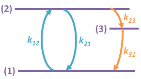
Figure 3: (Color online) Jablonski diagram of the three-level system, including the ground state (1), the excited state (2) and a metastable state (3). Only the allowed transition channels taken into account in the model are shown.

With $p_{i}$, $i=\{1,2,3\}$, the population of state $i$ we can write the following set of equations:

$$\dot{p_{1}}=-k_{12}p_{1}+k_{21}p_{2}+k_{31}p_{3},$$

$$\dot{p_{2}}=k_{12}p_{1}-(k_{21}+k_{23})p_{2},$$

$$\dot{p_{3}}=k_{23}p_{2}-k_{31}p_{3},$$

$$1=p_{1}+p_{2}+p_{3},$$ (7)

where $\dot{p_{i}}$ means time derivative of $p_{i}(t)$. The use of rate equations instead of Bloch equations is here fully justified since in ambient conditions, the coherence between levels is decaying very fast. Beveratos01b Eqs. 7 show that the system is necessarily in one of the states at any time. The steady-state analysis of these equations permits to find the explicit definition of the fluorescence rate $R$ at which the system emits photons. Novotny This definition allows us to explain the saturation behavior of the NV fluorescence, i.e., $R$ tends towards a finite value for increasing excitation power. However, we are here looking for the time-dependent analysis to find $p_{2}(\tau)$ as a function of the $k_{ij}$ coefficients. If we eliminate $p_{3}$ from Eq. 7, we obtain:

$$\dot{p_{1}}=-(k_{12}+k_{31})p_{1}+(k_{21}-k_{31})p_{2}+k_{31},$$

$$\dot{p_{2}}=k_{12}p_{1}-(k_{21}+k_{23})p_{2}.$$ (8)

The resolution of this pair of equations, with the initial conditions $p_{1}(0)=1$ and $p_{2}(0)=0$, leads to $p_{2}(\tau)=p(2,\tau|1,0)$ and therefore to the expression of $g^{(2)}(\tau)$.
Important approximations can be made to obtain a simple expression. More precisely, in addition to neglecting channels 1 to 3 and 3 to 2, we suppose that :

$$\{k_{21},k_{12}\}\gg\{k_{23},k_{31}\}.$$ (9)

This is justified since, even if the third level is considered, the associated rates are supposedly very small compared to the singlet rates $k_{12}$ and $k_{21}$. We will see latter that this is not really true for the NV^- center but that the results obtained are actually robust and keep their meaning even outside of their a priori validity range. Within the above mentioned approximations the second-order correlation function reads (see Appendix A for mathematical details):

$$g^{(2)}(\tau)=1-\beta e^{-\gamma_{1}\tau}+(\beta-1)e^{-\gamma_{2}\tau}\,,$$ (10)

where the parameters $\gamma_{1}$, $\gamma_{2}$ and $\beta$ are defined through the relations:

$$\gamma_{1}\simeq k_{12}+k_{21},$$ (11)

$$\gamma_{2}\simeq k_{31}+\dfrac{k_{12}k_{23}}{k_{12}+k_{21}},$$ (12)

$$\beta\simeq 1+\dfrac{k_{12}k_{23}}{k_{31}(k_{12}+k_{21})}.$$ (13)

III.2 Determination of the $k_{ij}$ coefficients

The aim of this sub-section is to determine the $k_{ij}$ coefficients for the specific measured NV centers. The fit to the $g^{(2)}(\tau)$ function allows us to determine $\gamma_{1}$, $\gamma_{2}$ and $\beta$. From Eqs. 11-13 we deduce:

$$k_{21}=\gamma_{1}-k_{12},$$ (14)

$$k_{31}=\dfrac{\gamma_{2}}{\beta},$$ (15)

$$k_{23}=\dfrac{\gamma_{1}\gamma_{2}(\beta-1)}{\beta k_{12}}.$$ (16)

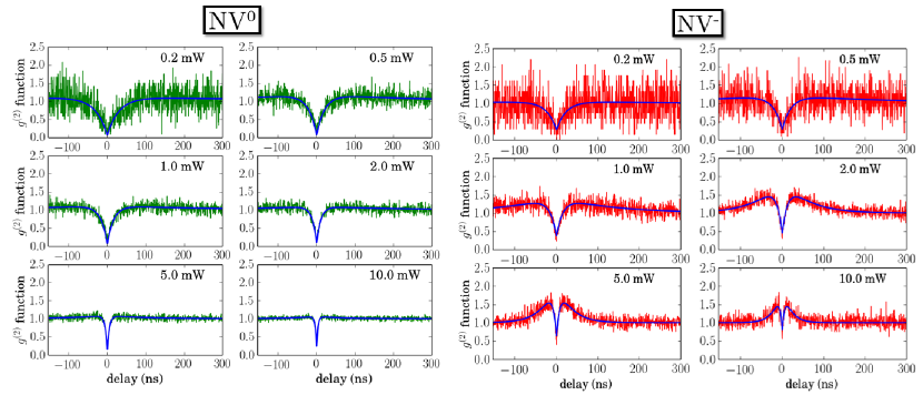
Figure 4: (Color online) Time-intensity second-order correlation functions $g^{(2)}(\tau)$ for a given NV⁰ center (green lines) and NV^- center (red lines). The excitation power is varied from 0.2 mW to 10 mW. The blue lines correspond to a three-level model fit.

We then have three equations for four unknown variables. A fourth equation is needed to solve the problem entirely. In the experiment, we also have access to the radiation or fluorescence rate $R$, measured in $s^{-1}$. This rate is simply the average number of photons that the APDs collect per second. It represents, up to a multiplicative coefficient associated with the photon propagation in the setup, the probability for the system to be in level 2, multiplied by the transition probability $k_{21}$ to relax (supposedly by optical means) to the ground state. We have:

$$R=\xi k_{21}p_{2}(+\infty),$$ (17)

where $\xi$ is the collection efficiency of the system once the NV center has emitted its fluorescence. Note that the same formula was used in refs. Kurtsiefer00 ; Beveratos01b with a different definition of $p_{2}(+\infty)$ because of a different Jablonski diagram. However, this has a physical meaning only if $k_{21}$ is associated with a pure radiative decay. Whereas the model of ref. Kurtsiefer00 ; Beveratos01b implied a unity quantum yield, the quantum yield in our approach is defined by

$$Q=\frac{k_{21}}{k_{21}+k_{23}}.$$ (18)

In our phenomenological approach the third level is thus assumed to absorb all of the non-radiative transitions letting $k_{21}$ be a pure radiative decay. Finally we remind that the probability $p_{2}(+\infty)$ needed in Eqs. 17 and 6 should be calculated in the asymptotic stationary regime, which can be obtained by canceling all $\dot{p_{i}}$ in Eq.8:

$$p_{2}(+\infty)=\frac{k_{31}}{-k_{21}+k_{31}+(k_{21}+k_{23})(1+k_{31}/k_{12})}.$$ (19)

Now four equations are at hand so that the system can be inverted to determine all coefficients. This calculation involves the numerical resolution through Cardano’s algorithm Cardano of a third-order polynomial as given in Appendix B.

IV Experimental results and extraction of the $k_{ij}$ parameters

We here consider two representative examples of NDs, one hosting a single pure NV^- center, and the second one hosting a single pure NV⁰ center. The NV^--center ND is about $25\leavevmode\nobreak\ nm$ in diameter, whereas the one hosting the NV⁰ center is about $50\leavevmode\nobreak\ nm$ in diameter. footnote The $g^{(2)}$ function was recorded for both NDs with different excitation powers $P_{exc}$ in order to study the evolution of the $k_{ij}$ coefficients.

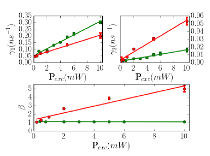
Figure 5: (Color online) Evolution of the $\gamma_{1}$, $\gamma_{2}$ and $\beta$ parameters as a function of the excitation power. Points are fits to the experimental $g^{(2)}$ functions using Eq. 10 and the lines are linear regressions. The green (red) points and lines correspond to the NV⁰ (NV^-) center. Errors bars are shown where they exceed the symbol size. They represent the standard deviation of each value calculated from the covariance matrix as given by the fitting routine.

Fig. 4 depicts the $g^{(2)}$ function for the two NV centers and for excitation powers $P_{exc}$ ranging from $200\leavevmode\nobreak\ \mu W$ to $10\leavevmode\nobreak\ mW$. The experimental curves are fitted with Eq. 10 taking into account the correction for the incoherent background light collected by the APDs. Brouri00 ; Sonnefraud08 ; Cuche09 The experimental antibunching dip does not drop to zero due to this incoherent background, which modifies Eq. 10 as $g_{\textrm{exp.}}^{(2)}(\tau)=g^{(2)}(\tau)\rho^{2}+1-\rho^{2}$ , where $\rho=S/(S+B)$ contains the signal $S$ and background $B$ contributions from the NV fluorescence and the spurious incoherent light, respectively. By recording the average intensity from the APD directly on the NV and at a location close to it, we experimentally determine $\rho$ and the fit parameters of Fig. 4 as explained in refs. Brouri00 ; Sonnefraud08 ; Cuche09 . It is seen that the increase of $P_{exc}$ only induces a very small bunching for the NV⁰, contrary to what is observed for the NV^-. However, the anti-bunching dip narrows with increasing power in both cases. Our observations are collected in Fig. 5, which shows the power evolution of the fit parameters $\gamma_{1}$, $\gamma_{2}$ and $\beta$.
The general trends seen in Fig. 4 are confirmed in Fig. 5 for both NVs since $\gamma_{1}$, which is associated with the antibunching contribution, is clearly increasing with $P_{exc}$, a fact which is reminiscent from Eq. 2. Furthermore, it is seen that $\gamma_{2}$ is also increasing significantly for the NV^- which is clear signature of the third energy level. As far as the $\beta$ parameter is concerned, it remains at a constant value $\beta\simeq 1$ for the NV⁰, while it increases up to $\beta\simeq 7$ for the NV^-. This behavior agrees with its definition from Eq. 10. Therefore, when $\beta$ is very close to 1, there is no significant bunching, and when $\beta$ increases with power, the bunching turns on.
Now that the three parameters have been found, the $k_{ij}$ parameters can be traced back. This will be done in two steps.

IV.1 $k_{ij}$ parameters with constant $k_{21}$

In Eq. 17 the collection efficiency $\xi$ of the optical setup must be known precisely to extract the various $k_{ij}$. However, since this can only be estimated, we will first calculate the $k_{ij}$ parameters by assuming that $k_{21}$ does not change with the excitation power. This hypothesis is intuitive because the parameter $k_{21}$, i.e., the spontaneous emission rate, is supposed to be solely governed by the Fermi’s golden rule, which in turn depends on the electromagnetic environment only. In order to determine the value of $k_{21}$ we observe that according to Eq. 14 we must have $\gamma_{1}=k_{21}$ at zero excitation since in this case $k_{12}=0$. From the linear regression for $\gamma_{1}$ (Fig. 5) we deduce $\gamma_{1}^{(0)}(P_{exc}=0)=k_{21}^{0}=0.052\leavevmode\nobreak\ ns^{-1}$ for the NV⁰, and $\gamma_{1}^{(-)}(P_{exc}=0)=k_{21}^{-}=0.046\leavevmode\nobreak\ ns^{-1}$ for the NV^- (here the (0) and (-) exponents refer to NV⁰ and NV^-, respectively). These constants give radiative lifetimes of $\tau_{21}^{(0)}=19.2\leavevmode\nobreak\ ns$ and $\tau_{21}^{(-)}=21.7\leavevmode\nobreak\ ns$, which are consistent with previous reports (see for example refs. Sonnefraud08 ; Beveratos01b ).

Figure 6: (Color online) Evolution of $k_{ij}$ parameters with power excitation when $k_{21}$ is fixed for (a) the NV⁰ and (b) for the NV^-. Errors bars are shown where they exceed the symbol size. These error bars are estimated from those of the $\gamma_{1}$, $\gamma_{2}$ and $\beta$ parameters, see Eqs. 14 to 16.

Thanks to Eqs. 14 to 16, we deduce the three other parameters as shown in Fig. 6 for both NVs. The first point to notice is that for both NVs, the $k_{12}$ parameter increases linearly with the pumping rate from zero to a value exceeding $k_{21}$ for $P_{exc}\simeq 2\leavevmode\nobreak\ mW$. Moreover, for NV⁰, we see that $k_{31}$ increases, but keeps very small values compared to the other parameters, in agreement with the assumptions made in Eq. 9. However, for NV^-, the same parameters are no longer negligible compared to the set of $k_{21}$, $k_{12}$ values. They even overtake $k_{21}$ for $P_{exc}>6\leavevmode\nobreak\ mW$. However, we emphasize that assuming $k_{21}$ constant, if natural, is actually not fully demonstrated. In order to check how robust this hypothesis is, we will now try to approach the values and evolutions of the $k_{ij}$ parameters that were obtained here by modulating the collection efficiency $\xi$ using Eq. 17.

IV.2 Modulation of the collection efficiency $\xi$

Now we use the fourth equation Eq. 17 to calculate the $k_{ij}$ parameters. As already stated, we do not know exactly the $\xi$ parameter but, as it turns out, slight variations in $\xi$ can produce significant changes in $k_{ij}$. To find the correct value of $\xi$, we adopt the following procedure. We let its value vary continuously and calculate the evolutions of the slope and Y-intercept of the linear regressions made with the obtained $k_{21}(P_{exc})$ traces. The slope should vanish because $k_{21}$ is assumed to be constant, whereas the Y-intercept should reach the value obtained previously, i.e., the value of $\gamma_{1}$ at zero excitation. Therefore, we calculate the evolution of the $k_{ij}$ parameters as a function of the collection efficiency $\xi$. The results are shown in Fig. 7, where the constant horizontal curves depict the values to be reached by the slope and Y-intercept. For the NV⁰ (Fig. 7 (a)), there is indeed a value of $\xi$ where the two parameters reach the assumed values (blue vertical line). This gives $\xi^{(0)}=0.77\times 10^{-3}$, in agreement with a rough estimate of our setup collection efficiency taking into account the various optical components.

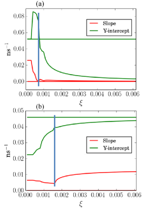
Figure 7: (Color online) Evolution of the slope and the Y-intersect of linear fit of $k_{21}(P_{exc})$ with the collection efficiency $\xi$ for the NV⁰ (a) and the NV^- (b). Straight lines are the values obtained previously with $k_{21}$ fixed.

However, for the NV^- (Fig. 7 (b)), it is seen that the parameters do not reach exactly the previous values. Yet, there is an optimum $\xi$ for which the $k_{ij}$ approach the previous values (blue vertical line). This corresponds to $\xi^{(-)}=1.6\times 10^{-3}$, which differs only by a factor 2 from the NV⁰ case. This appears reasonable since the measurements were not carried out the same day (optical alignments might be slightly different) and the collection efficiency $\xi$ also depends on the unknown transition-dipole orientation in both NVs.

IV.3 Comparaison of the photophysics of NV centers in both charge states

Fig. 8 depicts the $k_{ij}(P_{exc})$ curves deduced from the previous optimization. It is found that the order of magnitude of the coefficients is the same as for imposed $k_{21}$. In particular, the relaxation rate $k_{31}$ is unchanged because it only depends on the $g^{(2)}$ fit parameters, Eq. 15. For the two NV centers, the excitation rate vanishes in the absence of any excitation power and linearly increases with $P_{exc}$ as it should. The main difference between both centers comes from the evolution of $k_{23}$, $k_{31}$ and $k_{21}$. Indeed, for NV⁰, $k_{23}$ and $k_{31}$ remain very small compared to $k_{21}$, which is almost constant ($1/k_{31}\approx 500\leavevmode\nobreak\ ns$ and $1/k_{23}\approx 1000\leavevmode\nobreak\ ns$ if $P_{exc}$ tends to zero). Therefore, the third level plays little role in the photodynamics of the NV⁰ center. However, it is worth stressing that although very small, $k_{23}$ is not zero for NV⁰ (errors bars are within the symbol size in Fig. 8 (a), right panel), which confirms the very existence of the third metastable level for this charge state. Regarding the $g^{(2)}$ curves, it implies that the optical channel 2 to 1 is favored, which prevents any significant bunching. Furthermore, for the NV⁰ the narrowing of the antibunching dip is due to the increasing excitation rate as for a two-level system, i.e., Eq. 2 (see ref. Cuche09 ).

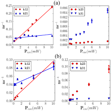
Figure 8: (Color online) Evolution of the $k_{ij}$ parameters with the excitation power taking into account the collection efficiency for the NV⁰ (a) and the NV^- (b) centers. Errors bars estimated as in Fig. 6 are shown where they exceed the symbol size.

The analysis of the $k_{ij}$ parameters for the NV^- is more involved. Indeed, $k_{23}$ increases very quickly to reach the order of magnitude of $k_{21}$, while the latter is increasing as well (at zero excitation power we have $1/k_{21}\simeq 24$ ns and $1/k_{23}\simeq 500$ ns). The increase of $k_{23}$, associated with non-radiative transitions, actually explains the growth of the bunching feature on the $g^{(2)}$ curves. Although the physical justification of this finding is beyond our phenomenological treatment, it is likely that the variation of $k_{21}$ and $k_{23}$ with excitation power is due to a change in the local energy environment of the NV center at high power, in particular because the efficient coupling with the phonon bath in the diamond matrix is expected to be temperature sensitive.

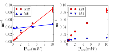
Figure 9: (Color online) Evolution of $k_{ij}$ parameters with power excitation taking into account the collection efficiency for the NV^- in the approximation-free rate-equation model. Errors bars estimated as in Fig. 6 are shown where they exceed the symbol size.

Increasing the excitation power could thus correspond to an increasing effective temperature, subsequently affecting the relaxation dynamics.
It is worth pointing out that there is a limitation in the analysis done for the NV^- center. Indeed, the very fact that $k_{23}$ and $\{k_{21},k_{12}\}$ reach the same order of magnitude contradicts the hypothesis made in Eqs. 9-13. Actually, as already mentioned, the results obtained are much more robust that could be anticipated at first sight. This can be figured out by relaxing the constraint of Eq. 9 as done in the detailed calculation presented in Appendix C. The results obtained with the new rate-equation model are shown in Fig. 9 for

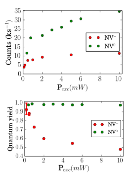
Figure 10: (Color online) Evolution of the fluorescence rate (upper panel) and the quantum yield $Q$ (lower panel) with the excitation power for the NV^- and NV⁰ center in the rate equation model free of any approximation. Errors bars for $Q$ are shown where they exceed the symbol size. They are estimated from those of the $k_{ij}$ parameters, see Eq. 18.

the evolution of the $k_{ij}$ coefficients of the NV^- center. The obtained values are very similar to those of the approximate treatment, thereby justifying the previous results. For the NV⁰ the coupling to the third level is very weak and the modifications (not shown) are even smaller.
To complete the analysis we also computed the quantum yield evolution as given by Eq. 18 and compared with the evolution of the fluorescence rate. Fig. 10 confirms that within the Jablonski model sketched in Fig. 3 and in the considered excitation regime, the quantum yield of the NV⁰ center is approximately constant $Q\simeq 1$, in agreement with the intuitive fact that the third level does not play a significant role in the dynamics. In contrast, the NV^- quantum yield decreases dramatically with increasing excitation power from a starting $Q\simeq 1$ to $Q\simeq 0.5$ at high power. This entails the fact that the NV^- dynamics is strongly dependent on the excitation power as discussed before.

V Photochromism

Photochromism of NV centers has been reported in ensembles of NV centers in CVD diamond films under additional selective illumination Iakoubovskii00 , with single NV centers in 90 nm NDs under femtosecond illumination, which results in the photo-ionization of the negative center to its neutral counterpart Dumeige04 , with ensembles of NV centers in type Ib bulk diamond at cryogenic temperatures under intense CW excitation Manson05 , and with a single center in natural type-IIa bulk diamond under CW illumination. Gaebel06 In this last report, a special scheme of cross-correlation photon measurements was applied in the emission band of both charge states to show that the collected fluorescence in the NV⁰ and NV^- states were correlated and originated form a single NV defect. Several studies have reported that charge conversion within the NVs critically depends on the illumination conditions. Waldherr ; beha ; aslam
A complete understanding of NV photochromism is lacking but a widespread view is that the optical excitation, either CW or transient, tunes the quasi Fermi level around a NV charge transition level, thereby inducing charge conversion. Iakoubovskii00 ; Grotz12 This scenario has been reinforced recently by electrical manipulation of the charge state of NV ensembles and of single NVs by an electrolytic gate electrode used to tune the Fermi energy. Grotz12 Depending on the sort of diamond studied, photochromism is thought to be favored by the presence of electron donor or acceptor defects, such as nitrogen, in the neighborhood of the NV center. Collins02 Recently, it was also found that resonant excitation of the NV⁰ and NV^- states in ultrapure synthetic IIa bulk diamond can induce reversible charge conversion in cryogenic conditions even at low power. Siyushev13 This was taken as evidence that the charge conversion process is intrinsic in this sort of diamond, not assisted by an electron donor or acceptor state. The goal of this section is to give additional information on NV photochromism detected in surface-purified NDs, 25 nm in size, subjected to a CW non-resonant excitation of increasing power. By comparing the behavior of a single photochromic center to that of non-photochromic centers in the same illumination conditions as described above, we gain valuable information on the rich photophysics of photochromism.
For the purpose of studying photochromism, we use two additional configurations of the HBT correlator that differ only by the set of bandpass filters added in the interferometer branches. These configurations, called NV^-/0, and NV^0/- respectively, are shown schematically in Fig. 11.

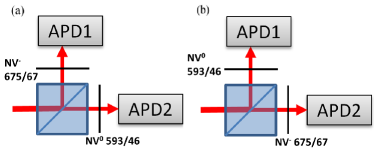
Figure 11: (Color online) HBT configurations used to study photochromism. (a) is the NV^-/0 configuration, where a bandpass filter (central wavelength 675 nm, bandwidth 67 nm) adapted to the negative NV^- center is inserted in the upper start branch, whereas a bandpass filter adapted to the neutral NV⁰ (central wavelength 593 nm, bandwidth 46 nm) is inserted in the lower stop branch. (b) is the NV^0/- configuration where both bandpass filters are interchanged compared to (a).

In contrast to Fig. 2(a), these two configurations add selective bandpass filters in the interferometer branches. The NV^-/0 configuration in Fig. 11 (a) (respectively NV^0/- configuration in Fig. 11 (b)) uses a filter selective to the NV^- (respectively NV⁰) fluorescence in the start (respectively stop) branch. Therefore, in the NV^-/0 configuration, a single photon emitted by a NV^- center and detected in APD1 gives the «  Start   » signal to the counting module, whereas a single NV⁰ photon subsequently detected in APD2 produces the «  Stop   » signal. The NV^0/- configuration works in just the complementary way. Note that our NV^-/0 configuration is similar to the cross-correlation technique used in ref.  Gaebel06 . These schemes turn out to be very powerful to study photochromism since cross correlation can be expected only if NV^- and NV⁰ photons originate from the same defect center. Note that related techniques have also successfully been applied to identify various excitonic species emitted by single semiconductor quantum dots, see for instance. Moreau01 ; Regelman01 ; Kiraz02 ; Couteau04 ; Sallen

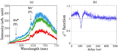
Figure 12: (Color online) (a) Fluorescence spectra of the photochromic ND nanoparticle taken at 3 different excitation powers of nominally 0.5 mW, 1 mW, 2 mW from bottom to top, respectively. (b) Antibunching curve at short time delays and an excitation power of 5 mW.

With the above setup, we have located a few rare NDs hosting a single NV center that showed charge conversion at low excitation power already. In the following, we consider such a ND hosting a single photochromic NV center.

The relevant spectra are shown in Fig. 12(a). It is found that both the NV⁰ and NV^- ZPLs are seen at any excitation power. The corresponding $g^{(2)}$ function measured in the standard configuration of the HBT (no bandpass filter) is shown in Fig. 12(b). It reveals a clear antibunching dip at zero delay. A precise analysis taking into account the background light (see Table 1) confirms this finding since at high excitation power we observe that the background $B$ increases significantly with respect with the NV fluorescence signal: $\rho=S/(S+B)\simeq 0.6$ while at low power $\rho\simeq 0.9-1$. With this value and using the formula $g_{\textrm{exp.}}^{(2)}(\tau)/\rho^{2}+1-1/\rho^{2}=g^{(2)}(\tau)$ we deduce the actual value of $g^{(2)}(0)\simeq 0$. Beveratos01 ; Sonnefraud08 ; Beveratos01b ; Hui09 From these results, a natural interpretation for the observation of the NV⁰ and NV^- ZPLs together with NV uniqueness is that this particular ND is subjected to photochromism. In addition to the antibunching dip at zero delay, it is seen in Fig. 12 that $g^{(2)}$ exceeds 1 at longer delays. Beveratos01b In agreement with the previous sections, this is evidence for the presence of a trapping level and calls for a three-level description of the photochromic NV. The values of $\gamma_{1}$, $\gamma_{2}$ and $\beta$ parameters used for fitting the $g_{\textrm{exp.}}^{(2)}$ function agree qualitatively well with those obtained for the NV^- considered previously in agreement with the fact that the system is acting more like a three-level system.
Although our study of NV photochromism is limited to a particular example we suggest that the dynamics of the system involves probably all energy levels of the NV^- and NV⁰ with some possible hybridization. It could be interesting to know, whether or not, the third level involved in the photochromic case is identical in nature to the third level of the NV^-. The role of the environment or of the radiation power TreussartPhysicaB2006 on the dynamics could be investigated in the future to clarify this point.

$P_{exc.}$(mW)	0.5	1	2	3	5
$R$(kHz)	11.8	17.1	23.0	27.7	32.0
$g_{\textrm{exp.}}^{(2)}(0)$	0.25	0.32	0.48	0.45	0.6
$S$(kHz)	10.2	14.1	16.6	20.5	20.2
$B$(kHz)	1.6	3.0	6.4	7.2	11.8
$\beta$	1.36	1.45	1.75	1.6	2.5
$\gamma_{1}$(ns-1)	0.03	0.036	0.044	0.052	0.054
$\gamma_{2}$(ns-1)	0.005	0.007	0.009	0.012	0.018

Table 1: Table summarizing the experimental parameters $P_{exc.}$, $R$, $g_{\textrm{exp.}}^{(2)}(0)$, $S$, $B$ measured on the photochromic NV for the observation of the $g_{\textrm{exp.}}^{(2)}$ function. The fit parameters $\gamma_{1}$,$\gamma_{2}$ and $\beta$ using a 3 energy-level model are also given.

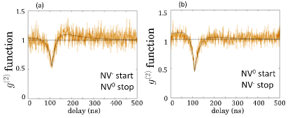
Figure 13: (Color online) Time-intensity second-order correlation functions measured for the photochromic NV center in two different HBT configurations. (a) is the cross correlation NV^-/0 configuration; (b) is the cross correlation NV^0/- configuration. The temporal window is [-100 ns; 500 ns] and the excitation power is 3 mW.

Switching now to the cross-correlation regime we show in Fig. 13 the result obtained for $P_{exc.}=3\leavevmode\nobreak\ mW$ (similar features, not shown here, were observed at other excitation powers). It is worth emphasizing that cross correlations, as described in e.g. refs. Aspect ; Regelman01 ; Kiraz02 , allow us to characterize the transitory dynamics between the two NV configurations. Using a formalism equivalent to the one leading to Eqs. 3-5 we indeed obtain in the NV^-/0 configuration sketched in Fig. 11 (a)

$$g^{(2)}_{-/0}(\tau)=\dfrac{p(e,\textrm{NV\fup{0}},t+\tau\lvert g,\textrm{NV\fup{-}},t)}{p(e,\textrm{NV\fup{-}},t)}$$ (20)

where $p(e,\textrm{NV\fup{0}},t+\tau\lvert g,\textrm{NV\fup{-}},t)$ is the conditional probability for the NV to be in the excited level $e$ of the NV⁰ state at time $t+\tau$ knowing that it was in the ground energy level $g$ of the NV^- charged state at the previous time $t$. This also means that a first photon emitted by the NV⁰ was detected at time $t$ while a second photon emitted by the NV^- is detected at time $t+\tau$ . In a symmetrical way using the NV^0/- configuration sketched in Fig. 11 (b) we get

$$g^{(2)}_{0/-}(\tau)=\dfrac{p(e,\textrm{NV\fup{-}},t+\tau\lvert g,\textrm{NV\fup{0}},t)}{p(e,\textrm{NV\fup{0}},t)}$$ (21)

with similar definitions as previously but with the role of NV⁰ and NV^- inverted.
The experimental results corresponding to these two configurations are shown in Figs. 13(a) and (b), respectively. Here, it is also important to have $\tau\geq 0$ in the calculation leading to Eqs. 20 and 21 in order to have a clear physical understanding. However, the electronic delay $\Delta=100$ ns included in the HBT correlator setup implies that sometimes even a photon emitted, say at time $t_{0}$, by a NV^- is recorded after a second photon emitted later by the NV⁰ state, i.e., at $t_{0}+\tau$. This corresponds to the ’negative’ delay part of the graph, i.e., Fig. 13(a), which is actually associated with the inverse dynamics NV^0/-, i.e., Eq. 21. Here for clarity we did not subtract the delay from the abscises in Fig. 13. Therefore for $\tau>\Delta$ in Fig. 13(a) we have $g^{(2)}_{exp.}(\tau)=g^{(2)}_{-/0}(\tau-\Delta)\rho^{2}+1-\rho^{2}$ while we have $g^{(2)}_{exp.}(\tau)=g^{(2)}_{0/-}(\Delta-\tau)\rho^{2}+1-\rho^{2}$ for $0<\tau<\Delta$ with $\rho=S/(S+B)$ as previously. In the same way for Fig. 13(b) we have $g^{(2)}_{exp.}(\tau)=g^{(2)}_{0/-}(\tau-\Delta)\rho^{2}+1-\rho^{2}$ for $\tau>\Delta$ and $g^{(2)}_{exp.}(\tau)=g^{(2)}_{-/0}(\Delta-\tau)\rho^{2}+1-\rho^{2}$ for $0<\tau<\Delta$.
As it is clear from the definitions these cross-correlations should present some symmetries. In the present case we used a three energy-level fit, i.e. Eq. 10, for the theoretical functions, Eqs. 20 and 21. The parameters obtained to reproduce the data are the same for Fig. 13 (a) and (b) up to an inversion between the ‘positive’ and ‘negative’ delay for each graph. Therefore, we get for Fig. 13(a) $\gamma_{1}=0.046\leavevmode\nobreak\ ns^{-1}$, $\gamma_{2}=0.01\leavevmode\nobreak\ ns^{-1}$ and $\beta=1.2$ for $\tau<\Delta$, while we have $\gamma_{1}=0.052\leavevmode\nobreak\ ns^{-1}$, $\gamma_{2}=0.01\leavevmode\nobreak\ ns^{-1}$ and $\beta=1.5$ for $\tau>\Delta$. For the second cross-correlation curve the parameters are identical but the roles of $\tau>\Delta$ and $\tau<\Delta$ are inverted as it should be. We observe that these values are very close to each other and also from the one obtained in Table 1 at the same excitation power $P_{exc.}=3\leavevmode\nobreak\ mW$. This confirms that the system acts here mainly as a NV^- center.
Interestingly, the last finding implies that after the emission of a photon in the spectral fluorescence band of the NV^- the delayed emission of a second photon in the spectral band of the NV⁰, i.e., the conditional probability given by Eq. 20, is also characterized by the dynamics of the NV^- contrary to the intuition. Such behavior was reported in ref. Gaebel06 for NV centers in bulk. In particular, in this paper the time dependence of the conversion NV⁰ to NV^- process (and its inverse) was studied using pulse sequences. It was found that the relaxation from NV^- to NV⁰ is a very slow process occurring with a decay time $\simeq 1\leavevmode\nobreak\ \mu s$. This agrees with our finding in Fig. 13 since, even if the full dynamics of the photochromic NV center is expected to depend on the energy levels of both the NV^- and NV⁰ centers, it is clearly the NV^- characteristics which dominate during the transition associated with Eq. 20. A similar qualitative analysis can be done in the NV⁰ to NV^- center conversion. The small dissymmetry between the two parts of the curves for positive and negative delays results from the presence of a small NV⁰ contribution to the dynamics during the NV⁰ to NV^- transition which is absent in the NV^- to NV⁰ conversion. Clearly, this complex charged/uncharged transition dynamics would deserve systematic studies in the future.

VI Summary

To summarize, we have experimentally studied the fluorescence photodynamics of NV^- and NV⁰ centers in diamond nanocrystals of 50 nm size or below using HBT photon-correlation measurements as a function of the excitation power. The dynamics was theoretically modeled using Einstein’s rate equations and the transition probability rates $k_{ij}$ entering the three-level model developed to analyze the data were deduced and used to infer a quantum efficiency to both charge states of the NV. It has been found that the shelving state, though present, plays a very small role on the neutral center in those small diamond crystals. The narrowing of the antibunching dip observed with increasing power for this center is a simple power effect that does not affect the near unity quantum efficiency. In contrast, the negative center experiences a distinctive photon bunching behavior at finite delay that increases with increasing power. This reflects the increasing role of the shelving state for this center, which in turn diminishes the quantum efficiency from near unity at low power to approximately 0.3 at high power. We have also studied the dynamics of a photochromic center. It reveals a rich phenomenology that is essentially dominated by the negative face of the center. In the future, it would be interesting to determine how the presence of, e.g., a plasmonic structure affects the dynamics of NV centers Schietinger09 in any charge state, in particular if the role of the shelving state in the NV⁰ center as well as the neutral face of the photochromic center can be modified.

VII Acknowledgments

This work was supported by Agence Nationale de la Recherche, France, through the NAPHO (grant ANR-08-NANO-054-01), PLACORE (grant ANR-13-BS10-0007) and SINPHONIE (grant ANR-12-NANO-0019) projects.

Annexe A

Here we briefly summarize the derivation of the main equations used in sections III and IV. We start from Eq. 8 written in a matrix form as

$$\dot{\mathbf{P}}:=\left(\begin{array}[]{c}\dot{p_{1}}\\ \dot{p_{2}}\end{array}\right)=\left(\begin{array}[]{cc}a&b\\ c&d\end{array}\right)\cdot\mathbf{P}+\mathbf{J}$$ (26)

$$=\mathbf{M}\cdot\mathbf{P}+\mathbf{J},$$ (27)

where

$$a=-(k_{12}+k_{13}+k_{31}),$$

$$b=k_{21}-k_{31},$$

$$c=k_{12}-k_{32},$$

$$d=-(k_{21}+k_{23}+k_{32}),$$

and

$$\mathbf{J}=\left(\begin{array}[]{c}k_{31}\\ k_{32}\end{array}\right).$$ (30)

For the sake of generality we here keep all transition coefficients $k_{ij}$ allowed by the three-level model. Such an Eq. 27 can be formally solved by defining a new vector $\mathbf{q}$ related to $\mathbf{P}$ by the equation $\mathbf{P}=e^{\mathbf{M}t}\cdot\mathbf{q}$. This leads to the new equation $\dot{\mathbf{q}}=e^{-\mathbf{M}t}\mathbf{J}$ which has the general solution:

$$\mathbf{q}(t)=\mathbf{q}(0)+\int_{0}^{t}d\tau e^{-\mathbf{M}\tau}\cdot\mathbf{J}$$

$$=\mathbf{q}(0)+\mathbf{M}^{-1}\cdot[1-e^{-\mathbf{M}t}]\cdot\mathbf{J}$$ (31)

where $\mathbf{M}^{-1}$ is the inverse matrix of $\mathbf{M}$ and where the initial condition corresponding to a system in the ground state at time $t=0$ is $\mathbf{q}(0)=\mathbf{P}(0)=\left(\begin{array}[]{c}1\\ 0\end{array}\right)$. Therefore, we deduce:

$$\mathbf{P}(t)=e^{\mathbf{M}t}\cdot(\mathbf{q}(0)+\mathbf{M}^{-1}\cdot[1-e^{-\mathbf{M}t}]\cdot\mathbf{J})$$ (32)

In order to give an explicit form to the solution we need to diagonalize the $\mathbf{M}$ matrix. Therefore, we write

$$\mathbf{\Pi}^{-1}\cdot\mathbf{M}\cdot\mathbf{\Pi}=\left(\begin{array}[]{cc}\lambda_{1}&0\\ 0&\lambda_{2}\end{array}\right).$$ (35)

The eigenvalues $\lambda_{1}$ and $\lambda_{2}$ of $\mathbf{M}$ are easily obtained from the secular equation $det[\mathbf{M-\lambda\mathbf{I}}]=0$. They reads:

$$\lambda_{1}=\frac{a+d}{2}-\frac{1}{2}\sqrt{[(a+d)^{2}-4det[\mathbf{M}]]}$$

$$\lambda_{2}=\frac{a+d}{2}+\frac{1}{2}\sqrt{[(a+d)^{2}-4det[\mathbf{M}]]}.$$ (36)

From Eq. 32 we easily obtain

$$\mathbf{\Pi}^{-1}\cdot\mathbf{P}=\left(\begin{array}[]{cc}e^{\lambda_{1}t}&0\\ 0&e^{\lambda_{2}t}\end{array}\right)\left(\begin{array}[]{c}\alpha\\ \varepsilon\end{array}\right)+\left(\begin{array}[]{c}\gamma\\ \delta\end{array}\right),$$ (43)

with

$$\left(\begin{array}[]{c}\gamma\\ \delta\end{array}\right)=-\left(\begin{array}[]{cc}1/\lambda_{1}&0\\ 0&1/\lambda_{2}\end{array}\right)\cdot\mathbf{\Pi}^{-1}\cdot\mathbf{J}$$ (48)

and

$$\left(\begin{array}[]{c}\alpha\\ \varepsilon\end{array}\right)=\mathbf{\Pi}^{-1}\cdot\left(\begin{array}[]{c}1\\ 0\end{array}\right)-\left(\begin{array}[]{c}\gamma\\ \delta\end{array}\right).$$ (55)

In order to determine completely the solution we need to specify the transformation matrix $\mathbf{\Pi}=\left(\begin{array}[]{cc}u_{1}&u_{2}\\ v_{1}&v_{2}\end{array}\right)$ whose column vectors $\mathbf{X}_{i}=\left(\begin{array}[]{c}u_{i}\\ v_{i}\end{array}\right)$ with $i=1,2$ are solutions of the eigenvalue problem $\mathbf{M}\cdot\mathbf{X}_{i}=\lambda_{i}\mathbf{X}_{i}$. These eingenvectors are determined up to an arbitrary normalization and here we choose

$$\mathbf{X}_{i}=\left(\begin{array}[]{c}b\\ \lambda_{i}-a\end{array}\right).$$ (58)

Using Eq. 43 we therefore get:

$$p_{2}(t)=v_{1}\alpha e^{\lambda_{1}t}+v_{2}\varepsilon e^{\lambda_{2}t}+v_{1}\gamma+v_{2}\delta.$$ (59)

We can further simplify the solution since from Eq. 55 and the definition of $M^{-1}$ we easily deduce $(v_{1}v_{2})\left(\begin{array}[]{c}\alpha\\ \varepsilon\end{array}\right)=-(v_{1}v_{2})\left(\begin{array}[]{c}\gamma\\ \delta\end{array}\right)$ , i.e., $v_{1}\alpha+v_{2}\varepsilon=-(v_{1}\gamma+v_{2}\delta)$. After regrouping all terms we obtain

$$\frac{p_{2}(t)}{p_{2}(\infty)}=-\frac{v_{1}\alpha}{v_{1}\alpha+v_{2}\varepsilon}e^{\lambda_{1}t}+(\frac{v_{1}\alpha}{v_{1}\alpha+v_{2}\varepsilon}-1)e^{\lambda_{2}t}+1$$

which up to notations is equivalent to Eq. 10 of Section III if we write $\lambda_{i}=-\gamma_{i}$ and $\beta=\frac{v_{1}\alpha}{v_{1}\alpha+v_{2}\varepsilon}$.

Annexe B

The results obtained in Appendix A are exact and no approximation were made for calculating the coefficients $\gamma_{i}$ and $\beta$. Now we will use the fact that $\{k_{21},k_{12}\}\gg\{k_{23},k_{31}\}$ to simplify and explicit these coefficients.
First, we point out that we have

$$\beta=\frac{(1-J_{1}/\gamma_{1})}{(\gamma_{1}-\gamma_{2})}\cdot\frac{\gamma_{1}\gamma_{2}}{J_{1}}$$

$$=\frac{(1-k_{31}/\gamma_{1})}{\sqrt{((a+d)^{2}-4det[\mathbf{M}])}}\frac{det[\mathbf{M}]}{k_{31}}.$$ (61)

Therefore from Eqs. 36 and 61 we see that all coefficients $\gamma_{i}$ and $\beta$ can be expressed as functions of $a+d$ and $det[\mathbf{M}]$. Up to the first order we have

$$a+d\simeq-(k_{12}+k_{21}),$$

$$det[\mathbf{M}]\simeq k_{31}(k_{12}+k_{21})+k_{23}k_{12},$$ (62)

Therefore, up to the same order, we have $\sqrt{((a+d)^{2}-4det[\mathbf{M}])}\simeq-(a+d)[1-4det[\mathbf{M}]/(a+d)^{2}]$. These lead to

$$\gamma_{1}\simeq-(a+d)=k_{12}+k_{21},$$

$$\gamma_{2}\simeq-\frac{det[\mathbf{M}]}{a+d}\simeq k_{31}+\frac{k_{23}k_{12}}{k_{12}+k_{21}},$$ (63)

which are Eqs. 11 and 12, respectively. Finally we have

$$\beta\simeq\frac{-1}{(a+d)}\frac{det[\mathbf{M}]}{k_{31}}\simeq 1+\frac{k_{23}k_{12}}{k_{31}(k_{12}+k_{21})}$$ (64)

which is Eq. 13.
In order to solve the system of equations 11-13 we first eliminate $k_{23}$ from Eq. 12 using Eq. 13, i.e.

$$k_{23}=\dfrac{\gamma_{1}k_{31}(\beta-1)}{k_{12}}.$$ (65)

Inserting this result into Eq. 11 leads to

$$k_{31}=\dfrac{\gamma_{2}}{\beta}$$ (66)

which constitutes our first parameter solution. In order to determine the other parameters we insert the value obtained for $k_{31}$ into Eq. 65 and Eq. 11 to obtain

$$k_{23}=\dfrac{\gamma_{1}\gamma_{2}(\beta-1)}{k_{12}\beta}$$

$$k_{21}=\gamma_{1}-k_{12}.$$ (67)

In other words, all parameters are now expressed as a function of the excitation coefficient $k_{12}$. To complete the solution we use Eqs. 17 and 19 for the single-photon rate $R$. After insertion of Eqs. 65 and 67 into Eq. 17 and some lengthly rearrangements we finally obtain

$$k_{12}^{3}-\gamma_{1}k_{12}^{2}+\frac{R}{\xi}(\gamma_{1}+\frac{X}{k_{31}})k_{12}+\frac{RX}{\xi}=0$$ (68)

with $X=(\beta-1)\gamma_{1}\gamma_{2}/\beta$. The three roots of this cubic equation can be obtained numerically using Cardano’s method.

Annexe C

We can generalize the analysis made in the previous Appendix B without any approximation. For this we first remark that we have the exact relations

$$\gamma_{1}\gamma_{2}=det[\mathbf{M}],$$

$$\gamma_{1}+\gamma_{2}=-(a+d),$$

$$R\cdot det[\mathbf{M}]=\xi k_{21}k_{12}k_{31}$$ (69)

which can be obtained after some manipulations from the definition of the M matrix and of Eqs. 17,19. If we now introduce the definitions

$$\begin{array}[]{c}A=det[\mathbf{M}]=(k_{12}+k_{21})k_{31}+(k_{12}+k_{31})k_{23},\\ B=-(a+d)-k_{31}=k_{12}+k_{21}+k_{23},\\ C=R\cdot det[\mathbf{M}]/\xi=k_{12}k_{21}\end{array}$$ (73)

we obtain after lengthly but straightforward calculations

$$k_{12}^{2}-Bk_{12}+C+A-Bk_{31}=0.$$ (74)

To complete the resolution of the system we use the exact relation Eq. 61. We finally obtain

$$\begin{array}[]{c}k_{31}=\gamma_{2}\gamma_{1}/[\gamma_{1}-\gamma_{2})\beta+\gamma_{2}],\\ k_{12}=B/2-\sqrt{[B^{2}-4(C+A-Bk_{31})]}/2,\\ k_{21}=C/k_{12},\\ k_{23}=B-k_{12}-k_{21}.\end{array}$$ (79)

The minus sign was chosen in the second equation for $k_{12}$ (i.e. solution of Eq. 74) since a Taylor expansion at low excitation power when $\gamma_{2}\ll\gamma_{1}$, $\beta\simeq 1$ gives for the two roots

$$k_{12}\simeq\gamma_{1}/2[1\pm\sqrt{(1-\frac{4R}{\xi\gamma_{1}})}]\simeq\gamma_{1}/2\pm\gamma_{1}/2\mp\frac{R}{\xi}.$$ (80)

In order to have the linear regime $k_{12}\propto R/\xi$ we must therefore impose the minus sign.

- (1) M. D. Eisaman, J. Fan, A. Migdall, and S. V. Polyakov, Rev. Sci. Instrum. 82, 071101 (2011).
- (2) A. Gruber, A. Dräbenstedt, C. Tietz, L. Fleury, J. Wrachtrup, and C. von Borczyskowski, Science 276, 2012 (1997).
- (3) S. Castelletto, I. Aharonovich, B. C. Gibson, B. C. Johnson, and S. Prawer, Phys. Rev. Lett. 105, 217403 (2010).
- (4) C. Wang, C. Kurtsiefer, H. Weinfurter, and B. Burchard, J. Phys. B: At. Mol. Opt. 39, 37 (2006); E. Neu, D. Steinmetz, J. Riedrich-Möller, S. Gsell, M. Fischer, M. Schreck, and C. Becher, New J. Phys. 13, 025012 (2011).
- (5) R. Brouri, A. Beveratos , J.-P. Poizat, and P. Grangier, Opt. Lett. 25, 1294 (2000).
- (6) Y. Sonnefraud, A. Cuche, O. Faklaris, J.-P. Boudou, T. Sauvage, J.-F. Roch, F. Treussart, and S. Huant, Opt. Lett. 33, 611 (2008)
- (7) Bleaching of NV centers has been reported in some very rare 5-nm nanodiamonds only, see: C. Bradac, T. Gaebel, N. Naidoo, M. J. Sellars, J. Twamley, L. J. Brown, A. S. Barnard, T. Plakhotnik, A. V. Zvyagin, and J. R. Rabeau, Nature Nanotech. 5, 345 (2010). These authors also reported on blinking of the NV emission in a minority (25%) part of their discrete ultrasmall nanodiamonds. This unusual blinking was demonstrated to arise from surface traps, not to photochromism as discussed in Section V of the present article, since the spectral signature of the blinking NVs remained of the NV- type, and did not show the NV0 feature.
- (8) G. Balasubramanian, P. Neumann, D. Twitchen, M. Markham, R. Kolesov, N. Mizuochi, J. Isoya, J. Achard, J. Beck, J. Tissler, V. Jacques, P. R. Hemmer, F. Jelezko, and J. Wrachtrup, Nature Mater. 8, 383 (2009)
- (9) L. Rondin, G. Dantelle, A. Slablab, F. Grosshans, F. Treussart, P. Bergonzo, S. Perruchas, T. Gacoin, M. Chaigneau, H.-C. Chang, V. Jacques, and J.-F. Roch, Phys. Rev. B 82, 115449 (2010).
- (10) P. Siyushev, H. Pinto, M. Vörös, A. Gali, F. Jelezko, and J. Wrachtrup, Phys. Rev. Lett. 110, 167402 (2013).
- (11) B. R. Smith, D. W. Inglis, B. Sandnes, J. R. Rabeau, A. V. Zvyagin, D. Gruber, C. J. Noble, R. Vogel, E. Osawa, and T. Plakhotnik, Small 5, 1649 (2009).
- (12) C. L. Degen, Appl. Phys. Lett. 92, 243111 (2008).
- (13) J. R. Maze, P. L. Stanwix, J. S. Hodges, S. Hong, J. M. Taylor, P. Cappellaro, L. Jiang, M. V. Gurudev Dutt, E. Togan, A. S. Zibrov, A. Yacoby, R. L. Walsworth, and M. D. Lukin, Nature (London) 455, 644 (2008).
- (14) G. Balasubramanian, I. Y. Chan, R. Kolesov, M. Al-Hmoud, J. Tisler, C. Shin, C. Kim, A. Wojcik, P. R. Hemmer, A. Krueger, T. Hanke, A. Leitenstorfer, R. Bratschitsch, F. Jelezko, and J. Wrachtrup, Nature (London) 455, 648 (2008).
- (15) P. Maletinsky, S. Hong, M. S. Grinolds, B. Hausmann, M. D. Lukin, R. L. Walsworth, M. Loncar, and A. Yacoby, Nature Nanotech. 7, 320 (2012).
- (16) L. Rondin, J.-P. Tetienne, P. Spinicelli, C. Dal Savio, K. Karrai, G. Dantelle, A. Thiaville, S. Rohart, J.-F. Roch, and V. Jacques, Appl. Phys. Lett. 100, 153118 (2012).
- (17) L. Rondin, J.-P. Tetienne, T. Hingant, J.-F. Roch, P. Maletinsky, and V. Jacques, Rep. Prog. Phys. 77, 056503 (2014).
- (18) M. S. Grinolds, S. Hong, P. Maletinsky, L. Luan, M. D. Lukin, R. L. Walsworth, and A. Yacoby, Nature Phys. 9, 215 (2013).
- (19) O. Faklaris, V. Joshi, T. Irinopoulou, P. Tauc, M. Sennour, H. Girard, C. Gesset, J.-C. Arnault, A. Thorel, J.-P. Boudou, P. A. Curmi, and F. Treussart, ACS Nano 3, 3955 (2009).
- (20) L. P. McGuinness, Y. Yan, A. Stacey, D. A. Simpson, L. T. Hall, D. Maclaurin, S. Prawer, P. Mulvaney, J. Wrachtrup, F. Caruso, R. E. Scholten, L. C. L. Hollenberg, Nature Nanotech. 6, 358 (2011).
- (21) D. I. Schuster, A. P. Sears, E. Ginossar, L. DiCarlo, L. Frunzio, J. J. L. Morton, H. Wu, G. A. D. Briggs, B. B. Buckley, D.D. Awschalom, and R. J. Schoelkopf, Phys. Rev. Lett. 105, 140501 (2010).
- (22) Y. Kubo, F. R. Ong, P. Bertet, D. Vion, V. Jacques, D. Zheng, A. Dréau, J.-F. Roch, A. Auffeves, F. Jelezko, J. Wrachtrup, M. F. Barthe, P. Bergonzo, and D. Esteve, Phys. Rev. Lett. 105, 140502 (2010).
- (23) O. Arcizet, V. Jacques, A. Siria, P. Poncharal, P. Vincent, and S. Seidelin, Nature Phys.7, 879 (2011).
- (24) S. Hong, M. S. Grinolds, P. Maletinsky, R. L. Walsworth, M. D. Lukin, and A. Yacoby, Nano Lett. 12, 3920 (2012).
- (25) A. Beveratos, R. Brouri, T. Gacoin, J.-P. Poizat, P. Grangier, Phys. Rev. A 64, 061802 (2001).
- (26) C. Kurtsiefer, S. Mayer, P. Zarda, and H. Weinfurter, Phys. Rev. Lett. 85, 290 (2000).
- (27) A. Sipahigil, M. L. Goldman, E. Togan, Y. Chu, M. Markham, D. J. Twitchen, A. S. Zibrov, A. Kubanek, and M. D. Lukin, Phys. Rev. Lett. 108, 143601 (2012).
- (28) S. Schietinger, M. Barth, T. Aichele, and O. Benson, Nano Lett. 9, 1694 (2009).
- (29) A. Cuche, A. Drezet, Y. Sonnefraud, O. Faklaris, F. Treussart, J.-F. Roch, and S. Huant, Opt. Express 17, 19969 (2009).
- (30) R. Beams, D. Smith, T. W. Johnson, S.-H. Oh, L. Novotny, and A. N. Vamivakas, Nano Lett. 13, 3807 (2013).
- (31) A. W. Schell, Ph. Engel, J. F. M. Werra, C. Wolff, K. Busch, and O. Benson, Nano Lett. 14, 2623 (2014).
- (32) R. Kolesov, B. Grotz, G. Balasubramanian, R. J. Stöhr, A. A. L. Nicolet, P. R. Hemmer, F. Jelezko, and J. Wrachtrup, Nature Phys. 5, 470 (2009).
- (33) A. Cuche, O. Mollet, A. Drezet, and S. Huant, Nano Lett. 10, 4566 (2010).
- (34) O. Mollet, S. Huant, G. Dantelle, T. Gacoin, and A. Drezet, Phys. Rev. B 86, 045401 (2012).
- (35) Y. Dumeige, F. Treussart, R. Alléaume, T. Gacoin, J.-F. Roch, and P. Grangier, J. Lumin. 109, 61 (2004).
- (36) T. Gaebel, M. Domhan, C. Wittmann, I. Popa, F. Jelezko, J. Rabeau, A. Greentree, S. Prawer, E. Trajkov, P. R. Hemmer, and J. Wrachtrup, Appl. Phys. B 82, 243 (2006).
- (37) G. Dantelle, A. Slablab, L. Rondin, F. Lainé, F. Carrel, P. Bergonzo, S. Perruchas, T. Gacoin, F. Treussart, and J.-F. Roch, J. Lumin. 130, 1655 (2010).
- (38) R. Loudon, The quantum theory of light (Oxford University Press, New York 2000).
- (39) L. Mandel and E. Wolf, Optical Coherence and Quantum Optics (Cambridge University Press, London, 1995).
- (40) H. J. Kimble and L. Mandel, Phys. Rev. A 13, 2123 (1973).
- (41) C. Kurtsiefer, P. Zarda, S. Mayer, and H. Weinfurter, J. Mod. Opt. 48, 2039 (2001).
- (42) M. W. Doherty, N. B. Manson, P. Delaney, F. Jelezko, J. Wrachtrup, L. C. Hollenberg, Phys. Rep. 528, 1 (2013).
- (43) M. W. Doherty, F. Dolde, H. Fedder, F. Jelezko, J. Wrachtrup, N. B. Manson, and L. C. Hollenberg Phys. Rev. B 85, 205203 (2012).
- (44) J. R. Maze, A. Gali, E. Togan, Y. Chu, A. Trifonov, E. Kaxiras, and M. D. Lukin, New J. Phys. 13, 025025 (2011).
- (45) A. Gali and J. R. Maze, Phys. Rev. B 88, 235205 (2013).
- (46) J.-P. Tetienne, L. Rondin, P. Spinicelli, M. Chipaux, T. Debuisschert, J.-F. Roch, and V. Jacques, New J. Phys. 14 103033 (2012).
- (47) P. Kehayias, M. W. Doherty, D. English, R. Fischer, A. Jarmola, K. Jensen, N. Leefer, P. Hemmer, N. B. Manson, and D. Budker, Phys. Rev. B 88, 165202 (2013).
- (48) A. Gali, Phys. Rev. B 79, 235210 (2009).
- (49) S. Felton, A. M. Edmonds, M. E. Newton, P. M. Martineau, D. Fisher, and D. J. Twitchen, Phys. Rev. B 77, 081201(R) (2008).
- (50) R. J. Glauber, Phys. Rev. 130, 2529 (1963).
- (51) P. W. Milonni, The quantum vacuum: an introduction to quantum electrodynamics (Academic Press, New-York, 1993).
- (52) Note that for the NV- center, one should consider a four-level model by including two intermediate singlet states Doherty1 ; delaney responsible for an additional ZPL line in the IR part of the spectrum. However, because of a rapid radiative decay between these states, only the low-energy singlet plays a role in the bunching behavior.
- (53) P. Dalaney, J. C. Greer, and J. A. Larsson, Nano Lett. 10, 610 (2010).
- (54) L. Novotny and B. Hecht, Principles of Nano-Optics (Cambridge University Press, London, 2006).
- (55) A. Beveratos, R. Brouri, J.-P. Poizat, P. Grangier, arXiv:quant-ph/0010044.
- (56) E. Rittweger, K.Y. Han, S. E Irvine, C. Eggeling, S. W. Hell, Nat. Photonics 3, 144 (2009).
- (57) G. Waldherr, J. Beck, M. Steiner, P. Neumann, A. Gali, Th. Frauenheim, F. Jelezko, and J. Wrachtrup, Phys. Rev. Lett. 106, 157601 (2011).
- (58) F. A. Inam, M. D. W. Grogan, M. Rollings, T. Gaebel, J. M. Say, C. Bradac, T. A. Birks, W. J. Wadsworth, S. Castelletto, J. R. Rabeau, and M. J. Steel, ACS Nano 7, 3833 (2013).
- (59) N. Jacobson, Basic Algebra I - 2nd edition (Dover, New-York, 2009).
- (60) These are nominal values. Because of the uncertainty on the exact location of the NV center in the ND matrix, we expect that the exact size of the studied NDs, whether 50 or 25 nm, is not a critical parameter in the present study.
- (61) K. Iakoubovskii, G. J. Adriaenssens, and M. Nasladek, J. Phys.: Cond. Matt. 12, 189 (2000).
- (62) N. B. Manson and J. P. Harrison, Diam. Relat. Mater. 14, 1705 (2005).
- (63) K. Beha, A. Batalov, N. B. Manson, R. Bratschitsch, and A. Leitenstorfer, Phys. Rev. Lett. 109, 097404 (2012).
- (64) N. Aslam, G. Waldherr, P. Neumann, F. Jelezko, New J. Phys. 15, 013064 (2013).
- (65) B. Grotz, M. V. Hauf, M. Dankerl, B. Naydenov, S. Pezzagna, J. Meijer, F. Jelezko, J. Wrachtrup, M. Stutzmann, F. Reinhard, and J. A. Garrido, Nat. Commun. 3, 729 (2012).
- (66) A. T. Collins, J. Phys.: Cond. Matt. 14, 3743 (2002).
- (67) E. Moreau, I. Robert, L. Manin, V. Thierry-Mieg, J.-M. Gérard, and I. Abram, Phys. Rev. Lett. 87, 183601 (2001).
- (68) D. V. Regelman, U. Mizrahi, D. Gershoni, E. Ehrenfreund, W. V. Schoenfeld, and P. M. Petroff, Phys. Rev. Lett. 87, 257401 (2001).
- (69) A. Kiraz, S. Fälth, C. Becher, B. Gayral, W.V. Schoenfeld, P.M Petroff, L. Zhang, E. Hu, A. Imamog̃lu, Phys. Rev. B 65, 161303 (2002).
- (70) C. Couteau, S. Moehl, F. Tinjod, J.-M. Gérard, K. Kheng, H. Mariette, J. A. Gaj, R. Romestain, and J.-P. Poizat, Appl. Phys. Lett. 85, 6251 (2004).
- (71) G. Sallen, A. Tribu, T. Aichele, R. André, L. Besombes, C. Bougerol, M. Richard, S. Tatarenko, K. Kheng, and J. P. Poizat, Nature Photon. 4,696 (2010).
- (72) Y. Y. Hui, Y.-R. Chang, T.-S. Lim, H.-Y. Lee, W. Fann, and H.-C. Chang, Appl. Phys. Lett. 94, 013104 (2009).
- (73) F. Treussart, V. Jacques, E. Wu, T. Gacoin, P. Grangier, J.-F. Roch, Physica B 376, 926 (2006).
- (74) A. Aspect, G. Roger, S. Reynaud, J. Dalibard, C. Cohen-Tannoudji, Phys. Rev. Lett. 45, 617 (1980).