Computing stress intensity factors for curvilinear cracks

Abstract

The use of the interaction integral to compute stress intensity factors around a crack tip requires selecting an auxiliary field and a material variation field. We formulate a family of these fields accounting for the curvilinear nature of cracks that, in conjunction with a discrete formulation of the interaction integral, yield optimally convergent stress intensity factors. We formulate three pairs of auxiliary and material variation fields chosen to yield a simple expression of the interaction integral for different classes of problems. The formulation accounts for crack face tractions and body forces. Distinct features of the fields are their ease of construction and implementation. The resulting stress intensity factors are observed converging at a rate that doubles the one of the stress field. We provide a sketch of the theoretical justification for the observed convergence rates, and discuss issues such as quadratures and domain approximations needed to attain such convergent behavior. Through two representative examples, a circular arc crack and a loaded power function crack, we illustrate the convergence rates of the computed stress intensity factors. The numerical results also show the independence of the method on the size of the domain of integration.

1 Introduction

The stress field near the tip of a loaded crack is singular under the assumption of linear elastic fracture mechanics. The coefficients of the asymptotic stress field, known as the stress intensity factors, play a key role in characterizing the magnitude of the load applied to the crack and predicting its propagation.

Given the stress singularity and the poor accuracy in pointwise evaluation of the stress field, it is often impossible to extract the stress intensity factors directly from numerical solutions, unless a higher-order method to compute the elastic field is adopted, such as those proposed in Liu et al. [1], Shen and Lew [2], and Chiaramonte et al. [3].

As a result, path and domain integral methods to extract the stress intensity factors have been created precisely to circumvent this limitation. A method of this kind typically formulates the expression of the stress intensity factors as functionals of the solution, thus enjoying a higher order of convergence than the one of the elastic field itself. Predominant methods of this kind have been constructed based on the $J$-integral [4] and the interaction integral [5].

In the context of linear elastic fracture mechanics, the $J$-integral is identified with the system’s elastic energy release rate; the elastic energy that would be released per unit length of crack extension in the tangential direction. This integral and related ones for the computation of fracture-mechanics-related quantities have been elaborated by Eshelby eshelby1951 [6], Rice [4], Freund [7], and many others. Shih et al. [8] derived the expression for the energy release rate of a thermally stressed body in the presence of crack face traction and body force. A general treatment of such conservation integrals, including those expressed in a form of domain integrals, can be found in Moran and Shih moran1987a [9, 10]. The domain form is better suited and more accurate for numerical computation. Nevertheless, in the case of mixed-mode loading, $J$ is a quadratic function of all three stress intensity factors [11]; therefore, additional integrals are needed to determine the three quantities individually, e.g., as done by Chang and Wu [12] for non-planar curved cracks.

In contrast, the interaction integral, or the interaction energy integral, is able to yield the three stress intensity factors separately. This method is based on the $J$-integral by superposing the elastic field of the loaded body and an auxiliary field with known stress intensity factors. The auxiliary field does not need to satisfy the elasticity equations but must resemble the asymptotic solution of a cracked elastic body corresponding to one of the three loading modes (e.g., plane-strain mode I or mode II, or anti-plane mode III). Therefore the auxiliary field, for straight cracks, is normally chosen to be the asymptotic solution, as found in [13, 14]. Doing so readily yields the stress intensity factor of the actual field for the chosen mode. Along with the auxiliary field, the interaction integral requires the construction of a vector field, named the material variation field, which indicates the velocity (variation) of points in the reference configuration as it is deformed into a domain with a longer crack. Under mild conditions, the value of the interaction integral does not depend on this choice, but a good choice of material variation can simplify computations. For example, the interaction integral is computed by integrating over the support of the material variation field, so it is convenient to choose material variation fields with small and compact support. While developing auxiliary and material variation fields for straight cracks (planar cracks in three dimension) is an amenable task, doing so for curvilinear cracks (non-planar cracks in three dimension) poses several challenges. In the following paragraphs we provide a short review of the effort related to the computation of stress intensity factors with the use of the interaction integral.

Earlier methods to compute the stress intensity factors with the interaction integral involved path integrals, such as those in Stern et al. [5] and Yau et al. [15]. The method was later generalized to a straight-front crack in three-dimensions by Nakamura and Parks [16] and Nakamura [17]. A curved crack front introduces additional terms, since the popular plane-strain modes I and II auxiliary fields no longer satisfy the compatibility and the equilibrium conditions. These additional terms were accounted for in Nahta and Moran [18] for the axisymmetric case, and in Gosz et al. gosz1998 [19] for general planar cracks in three dimensions. Kim et al. [20] adopted auxiliary fields corresponding to penny-shaped cracks, as well as conventional plane-strain and anti-plane ones. An alternative approach was given by Daimon and Okada [21] who adopted a compatible auxiliary field and accounted for its lack of equilibrium by superposing a numerically computed displacement field with the finite element method. A study of the effect of omitting some terms accounting for the curved front is given by Walters et al. [22].

More recently the method of gosz1998 [19] was adapted for non-planar cracks in Gosz and Moran [23], the latter of which is arguably a milestone in the development of domain integral methods to extract stress intensity factors from curvilinear cracks in 2D and non-planar cracks in 3D. In [23], the method constructs the auxiliary fields through the use of curvilinear coordinates and their corresponding covariant basis to account for the crack curvature. This procedure constructs the auxiliary fields by juxtaposing the components of the stress fields of williams1952 [13] with the described basis. In [24], Sukumar et al. implemented the method of [23] in combination with an extended finite element method in a three-dimensional setting [25] and a fast-marching method. The main drawback of the curvilinear coordinates of [23] is the need to perform boundary integrals over both the real crack surfaces and a pair of fictitious crack surfaces. In [26], González-Albuixech et al. proposed another curvilinear coordinate system that can eliminate the integration on the fictitious crack surfaces, and in this way facilitate the computation.

In [27, 26], González-Albuixech et al. studied the properties of the aforementioned methods in two- and three-dimensions, respectively, but not with all terms arising from the derivation of the interaction integral. Such omission of terms may have contributed to the observed slow convergence and occasional divergence. This observation confirms the statement of [23] that all terms arising from the lack of compatibility and equilibrium of the auxiliary field have to be taken into account.

The domain version of the interaction integral has also been generalized to functionally graded materials [28, 29].

In this paper we present a suite of auxiliary fields and material variations fields. By pairing two constructs of material variation fields and two constructs of auxiliary fields, we create two kinds of interaction integral suitable for curvilinear cracks and for situations in which body forces and crack face tractions are present. One kind of interaction integral is suited for applications where crack faces are loaded (e.g. hydraulic fracturing), and the other one is best suited for applications where body forces are non-zero (e.g. thermally loaded materials). Moreover, no fictitious crack face is needed, a major simplification to the predominant method in the literature.

One of the two choices of the material variation fields has a constant direction pointing to the direction of the crack growth, a straightforward choice adopted by most authors, and the other has a direction that is tangential to the crack near the crack tip, similar to that proposed in [25]. For a curved crack, this second choice necessarily coincides with the first one only at the crack tip. A key advantage of the material variation fields we introduce here is their ease of construction which is reflected in their straightforward implementation in computer codes. Moreover, in contrast to many of the existing constructions, the magnitude of the material variation fields is mesh independent. This mesh independence contributes to the observed optimal rate of convergence.

The two auxiliary fields are constructed from the well-known asymptotic solutions of a straight crack. Both fields respect the discontinuity introduced by the crack, thus avoiding the evaluation of integrals over fictitious crack faces as the method in [23] does. One of the auxiliary fields is obtained by “extending” the asymptotic solutions past the range $[-\pi,\pi]$, and hence satisfies equilibrium, compatibility, and the constitutive relation. The resulting interaction integral expression then yields a term on the crack faces, even in the absence of crack face traction. The second auxiliary field is an incompatible strain field. It is obtained by first mapping a straight crack to the curved crack near the crack tip, and using this map to push forward the strain field of the straight-crack asymptotic solution. Then, by suitably rotating the strain tensor at each point, we obtain an auxiliary strain field that is traction-free at the curved crack faces. This is useful for problems in which crack faces are traction-free. In fact, if this auxiliary field is used in combination with the tangential material variation field, the crack face integral vanishes, resulting in a significantly simplified expression for the interaction integral.

We showcase the convergence of the stress intensity factors obtained with the proposed fields for a set of representative examples computed with two different finite element methods. In all cases, the stress intensity factors converge with a rate that doubles the rate of convergence of the strains. We also numerically demonstrate the independence of the computed stress intensity factors from the chosen support for the material variation field. Although the numerical examples adopt finite element methods to obtain an approximate solution to the elasticity problem, the numerical implementation of the interaction integral with the new fields is general, and can be used in conjunction with any numerical method for the solution of the governing equations (e.g. finite difference, finite volume, boundary integral equations, isogeometric analysis, and meshless methods).

The paper is organized as follows. We first state the problem that we seek to solve in §2. We then proceed in §3 to present the interaction integral with the description of the new material variation and auxiliary fields. In the same section we justify that the proposed forms of the interaction integral are well-defined. A numerical approximation of the interaction integral is presented in §4 with remarks on its expected convergence. The last part of §4 provides a step-by-step recapitulation of the method suited for the reader interested in a concise presentation. In §5 we verify the computation of the stress intensity factors against analytical solutions for two problems: a circular arc crack and a power function crack. Throughout the paper we included sections titled “Justification” which contain sketches of proofs for some of the assertions we make, and they are not essential for the description of the methods in this paper.

2 Problem Statement

We present next the problem statement which consists of the evaluation of the stress intensity factors following the solution of the elasticity fields for a cracked solid.

2.1 Elasticity Problem

We consider a body $\mathcal{B}\subset\mathbb{R}^{2}$ undergoing a deformation defined by the displacement field ${\boldsymbol{u}}$. We assume $\mathcal{B}$ to be an open and connected domain with a (piecewise) smooth boundary $\partial\mathcal{B}$. We represent the crack with a twice differentiable, simple and rectifiable curve $\mathscr{C}\subset\mathcal{B}$ and denote its crack faces with $\mathscr{C}_{\pm}$. The cracked domain is given by $\mathcal{B}_{\mathscr{C}}=\mathcal{B}\backslash\mathscr{C}$. The boundary of $\mathcal{B}_{\mathscr{C}}$ is the union of the crack faces and the boundary of $\mathcal{B}$, namely $\partial\mathcal{B}_{\mathscr{C}}=\partial\mathcal{B}\cup\mathscr{C}_{\pm}$. Let $\partial\mathcal{B}_{\mathscr{C}}$ be decomposed into $\partial_{\tau}\mathcal{B}_{\mathscr{C}}$ and $\partial_{d}\mathcal{B}_{\mathscr{C}}$ such that $\partial_{\tau}\mathcal{B}_{\mathscr{C}}\supseteq\mathscr{C}_{\pm}$, $\partial_{\tau}\mathcal{B}_{\mathscr{C}}\cup\partial_{d}\mathcal{B}_{\mathscr{C}}=\partial\mathcal{B}_{\mathscr{C}}$, and $\partial_{\tau}\mathcal{B}_{\mathscr{C}}\cap\partial_{d}\mathcal{B}_{\mathscr{C}}=\emptyset$. Tractions $\overline{\boldsymbol{t}}$ and displacements $\overline{\boldsymbol{u}}$ are prescribed over $\partial_{\tau}\mathcal{B}_{\mathscr{C}}$ and $\partial_{d}\mathcal{B}_{\mathscr{C}}$, respectively, while a body force field ${\boldsymbol{b}}$ is applied over $\mathcal{B}_{\mathscr{C}}$. Let $\boldsymbol{x}_{t}$ denote any one of the two crack tips. We denote by ${\boldsymbol{n}}$ the unit external normal to ${\cal B}$, as well as the unit external normal to each one of the two faces of the crack. Figure 1 shows the schematic of the problem configuration.

Figure 1: The configuration of the problem

We confine ourselves to planar linear elasticity in the context of infinitesimal deformations. The elasticity problem statement reads: Given ${\boldsymbol{b}}$ , $\overline{\boldsymbol{u}}$, and $\overline{\boldsymbol{t}}$ find ${\boldsymbol{u}}:\mathcal{B}_{\mathscr{C}}\to\mathbb{R}^{2}$ such that

$$\nabla\cdot\boldsymbol{\sigma}(\nabla{\boldsymbol{u}})+{\boldsymbol{b}} =0,\quad \text{ in }\mathcal{B}_{\mathscr{C}},$$ (1a)

$${\boldsymbol{u}} =\overline{\boldsymbol{u}},\quad \text{ on }\partial_{d}\mathcal{B}_{\mathscr{C}},$$ (1b)

$$\boldsymbol{\sigma}(\nabla{\boldsymbol{u}}){\boldsymbol{n}} =\overline{\boldsymbol{t}},\quad \text{ on }\partial_{\tau}\mathcal{B}_{\mathscr{C}},$$ (1c)

where $\boldsymbol{\sigma}$ is the stress tensor. This is given by

$$\boldsymbol{\sigma}(\nabla{\boldsymbol{u}})=\mathbb{C}:\nabla{\boldsymbol{u}},$$ (2)

and

$$\mathbb{C}=\hat{\lambda}{\bf 1}\otimes{\bf 1}+2\mu\mathbb{I},\hbox{\hskip 14.45377pt}\hat{\lambda}=\begin{cases}\lambda,&\text{ for plane strain},\\ \dfrac{2\lambda\mu}{\lambda+2\mu},&\text{ for plane stress}.\end{cases}$$

The constants $\lambda$ and $\mu$ are Lamé’s first and second parameters, respectively, ${\bf 1}$ is the identity second-order tensor, and $\mathbb{I}$ is the fourth-order symmetric identity operator given by

$$\mathbb{I}=\frac{1}{2}(\delta_{ik}\delta_{jl}+\delta_{il}\delta_{jk}){\boldsymbol{e}}_{i}\otimes{\boldsymbol{e}}_{j}\otimes{\boldsymbol{e}}_{k}\otimes{\boldsymbol{e}}_{l},$$

where $\{{\boldsymbol{e}}_{1},{\boldsymbol{e}}_{2}\}$ is a Cartesian basis, and an index repeated twice indicates sum from 1 to 2 in such index.

2.2 Crack Tip Coordinates and Stress Intensity Factors

To aid the definition of the stress intensity factors we first introduce a system of coordinates and a family of vector bases.

Figure 2: Description of local basis and coordinates

Let $(r,\vartheta)$ be crack tip polar coordinates as shown in Fig. 2, and let $B_{\rho}(\hat{\boldsymbol{x}})=\left\{\boldsymbol{x}\in\mathbb{R}^{2}\middle||\boldsymbol{x}-\hat{\boldsymbol{x}}|<\rho\right\}$ be the open ball of radius $\rho>0$ centered at $\hat{\boldsymbol{x}}$. The radial coordinate is defined as $r(\boldsymbol{x}):=|\boldsymbol{x}-\boldsymbol{x}_{t}|$. Let $\Gamma:r\mapsto\{\boldsymbol{x}\in\mathscr{C}|\;|\boldsymbol{x}-\boldsymbol{x}_{t}|=r\}$ be a description of part of the crack parametrized by the distance to the crack tip. We set the domain of $\Gamma$ to be $[0,\rho]$ with $\rho>0$ such that $B_{\rho}(\boldsymbol{x}_{t})\subset\mathcal{B}$ and that $\Gamma^{\prime}\neq 0$ over its domain of definition. As a consequence, $\Gamma$ is bijective for $r\in[0,\rho]$. We re-iterate that the crack is assumed to be a twice continuously differentiable curve such that $\Gamma\in C^{2}(\mathbb{R}_{0}^{+};\mathbb{R}^{2})$, where $\mathbb{R}_{0}^{+}=\{0\}\cup\mathbb{R}^{+}$. By convention, the possible values of the $(r,\vartheta)$ coordinates for points in $B_{\rho}(\boldsymbol{x}_{t})$ that we will use belong to

$$D_{\rho}=\{(r,\vartheta)\in\mathbb{R}_{0}^{+}\times\mathbb{R}\mid-\pi-\zeta(r)\leq\vartheta\leq\pi-\zeta(r)\},$$

where $\zeta(r)$ is the angle between the vector $\Gamma(r)-\boldsymbol{x}_{t}$ and $\Gamma^{\prime}(0)$. In other words, $\zeta(r)$ is the angle subdued by (a) the tangent at the crack tip and (b) the secant line passing through the crack tip and $\Gamma(r)$. Figure 3 shows the values of the coordinate $\vartheta$ for the particular case of a circular arc crack. Lastly let ${\boldsymbol{g}}_{i}(r),r\in[0,\rho]$ be the right-handed orthonormal bases induced from the mapping $\Gamma$ such that ${\boldsymbol{g}}_{1}(r)=-\Gamma^{\prime}(r)/|\Gamma^{\prime}(r)|$, see Fig. 2.

Figure 3: The $\vartheta$-coordinate with the branch cut along the crack.

Throughout this manuscript, we assume that there exist unique real numbers $K_{I},K_{II}$ such that

$${\boldsymbol{u}}=K_{I}{\boldsymbol{u}}^{I}+K_{II}{\boldsymbol{u}}^{II}+{\boldsymbol{u}}_{S},\quad{\boldsymbol{u}}_{S}\in H^{2}\left(\mathcal{B}_{\mathscr{C}};\mathbb{R}^{2}\right),$$ (3)

where $K_{I}$ and $K_{II}$ are the modes $I$ and $II$ stress intensity factors, respectively, and ${\boldsymbol{u}}^{I},{\boldsymbol{u}}^{II}\in H^{1}(\mathcal{B}_{\mathscr{C}};\mathbb{R}^{2})\setminus H^{2}(\mathcal{B}_{\mathscr{C}};\mathbb{R}^{2})$ are the asymptotic displacement solutions of these modes.

The problem of evaluating the stress intensity factors is: Given a solution ${\boldsymbol{u}}$ of Problem (1), compute $K_{I}$ and $K_{II}$ as defined in (3).

Remark (Explicit evaluation of the behavior at the crack tip). Whenever $\boldsymbol{\beta}=\nabla{\boldsymbol{u}}\in C^{0}(\mathcal{B}_{\mathscr{C}};\mathbb{R}^{2\times 2})$, the stress intensity factors can be alternatively defined as:

$$K_{I}=\lim_{r\to 0}\sqrt{2\pi r}\boldsymbol{\sigma}(\boldsymbol{\beta})|_{\vartheta=0}:{\boldsymbol{g}}_{2}\otimes{\boldsymbol{g}}_{2},$$ (4)

$$K_{II}=\lim_{r\to 0}\sqrt{2\pi r}\boldsymbol{\sigma}(\boldsymbol{\beta})|_{\vartheta=0}:{\boldsymbol{g}}_{1}\otimes{\boldsymbol{g}}_{2}.$$

The calculation of the stress intensity factors by evaluating the limits in (4) with a numerical solution often leads to poor results. In fact, few methods are capable of accurately resolving the singularity in the stress field. Therefore the predominant methods to compute the stress intensity factors are based on the approximation of the interaction integral, a formulation that avoids pointwise evaluation of the stress field in the region with the singularity. We proceed to introduce the interaction integral in §3.

3 Interaction Integral

In the sequel we first define the interaction integral functional between any two admissible fields alongside a concise justification of this definition (see §3.1 ). In §3.2 we specialize it to the case in which one of the fields is the solution to the elasticity problem of interest. This specialization results in a formulation that possesses the following properties: (a) it does not involve second derivatives of the discrete approximation to the exact displacement field; (b) it is a problem-dependent functional because it uses the prescribed tractions and body forces; and (c) it can be further simplified, depending on the problem, by carefully choosing the so-called material variation and auxiliary fields, to be described later. We perform the simplification in §3.3 and §3.4, and obtain three different formulas. In §3.5 we provide guidelines on which specific formula for the interaction integral to choose for a given application.

3.1 Definition of the Interaction Integral Functional

The interaction integral involves two elasticity fields, one with known stress intensity factors, and the other whose stress intensity factors we are interested in evaluating.

Let us introduce the interaction energy momentum tensor $\overline{\boldsymbol{\Sigma}}:\mathbb{R}^{2\times 2}\times\mathbb{R}^{2\times 2}\to\mathbb{R}^{2\times 2}$ defined as

$$\overline{\boldsymbol{\Sigma}}\left(\boldsymbol{\beta}^{a},\boldsymbol{\beta}^{b}\right)=\overline{w}\left(\boldsymbol{\beta}^{a},\boldsymbol{\beta}^{b}\right){\bf 1}-\boldsymbol{\beta}^{a}\,{}^{\top}\boldsymbol{\sigma}\left(\boldsymbol{\beta}^{b}\right)-\boldsymbol{\beta}^{b}\,{}^{\top}\boldsymbol{\sigma}(\boldsymbol{\beta}^{a}),\\$$

where $\overline{w}:\mathbb{R}^{2\times 2}\times\mathbb{R}^{2\times 2}\to\mathbb{R}$ is given as

$$\overline{w}\left(\boldsymbol{\beta}^{a},\boldsymbol{\beta}^{b}\right)=\frac{1}{2}\left[\boldsymbol{\sigma}(\boldsymbol{\beta}^{a}):\boldsymbol{\beta}^{b}+\boldsymbol{\sigma}\left(\boldsymbol{\beta}^{b}\right):\boldsymbol{\beta}^{a}\right].$$ (5)

Assuming the same constitutive relation (2) for both fields, (5) simplifies to

$$\overline{w}\left(\boldsymbol{\beta}^{a},\boldsymbol{\beta}^{b}\right)=\boldsymbol{\sigma}(\boldsymbol{\beta}^{a}):\boldsymbol{\beta}^{b}=\boldsymbol{\sigma}\left(\boldsymbol{\beta}^{b}\right):\boldsymbol{\beta}^{a}.$$

Additionally, let the set of material variations be defined as

$$\mathcal{M}=\left\{\delta\boldsymbol{\gamma}\in{C^{1}\left(\mathcal{B}_{\mathscr{C}};\mathbb{R}^{2}\right)}\,\middle|\delta\boldsymbol{\gamma}={\bf 0}\text{ in }\mathcal{B}_{\mathscr{C}}\setminus B_{\rho}(\boldsymbol{x}_{t}),\delta\boldsymbol{\gamma}(\boldsymbol{x}_{t})={\boldsymbol{g}}_{1}(0)\right\}.$$ (6)

Finally, let

$$\mathscr{B}^{b}=\operatorname{span}\left\{\nabla{\boldsymbol{u}}^{I},\nabla{\boldsymbol{u}}^{II}\right\}\oplus H^{1}\left(\mathcal{B}_{\mathscr{C}};\mathbb{R}^{2\times 2}\right),$$

and for any tensor field $\boldsymbol{\beta}\in\mathscr{B}^{b}$ define $K_{I}[\boldsymbol{\beta}]$ and $K_{II}[\boldsymbol{\beta}]$ such that

$$\boldsymbol{\beta}=K_{I}[\boldsymbol{\beta}]\nabla{\boldsymbol{u}}^{I}+K_{II}[\boldsymbol{\beta}]\nabla{\boldsymbol{u}}^{II}+\boldsymbol{\beta}_{S}$$ (7)

with $\boldsymbol{\beta}_{S}\in H^{1}\left(\mathcal{B}_{\mathscr{C}};\mathbb{R}^{2\times 2}\right)$. In particular, if $\boldsymbol{\beta}=\nabla{\boldsymbol{u}}$, for ${\boldsymbol{u}}$ being a solution of Problem (1), then $K_{I}[\boldsymbol{\beta}]$ and $K_{II}[\boldsymbol{\beta}]$ are the stress intensity factors of ${\boldsymbol{u}}$. However, $K_{I}[\boldsymbol{\beta}]$ and $K_{II}[\boldsymbol{\beta}]$ are still defined for any $\boldsymbol{\beta}\in\mathscr{B}^{b}$ that is not the gradient of a displacement field. For convenience, regardless of whether $\boldsymbol{\beta}$ is or is not the gradient of a displacement field, we will refer to $K_{I}[\boldsymbol{\beta}]$ and $K_{II}[\boldsymbol{\beta}]$ as the stress intensity factors of $\boldsymbol{\beta}$.

We define the interaction integral functional $\hat{\mathcal{I}}:\mathscr{B}^{b}\times\mathscr{B}^{b}\times\mathcal{M}\to\mathbb{R}$ as

$$\hat{\mathcal{I}}\left[\boldsymbol{\beta}^{a},\boldsymbol{\beta}^{b},\delta\boldsymbol{\gamma}\right]= \int_{\mathscr{C}^{\pm}_{\rho}}\delta\boldsymbol{\gamma}\cdot\overline{\boldsymbol{\Sigma}}\left(\boldsymbol{\beta}^{a},\boldsymbol{\beta}^{b}\right){\boldsymbol{n}}\;dS$$ (8)

$$- \int_{B_{\rho}(\boldsymbol{x}_{t})\setminus\mathscr{C}}\left[\overline{\boldsymbol{\Sigma}}\left(\boldsymbol{\beta}^{a},\boldsymbol{\beta}^{b}\right):\nabla\delta\boldsymbol{\gamma}+\nabla\cdot\overline{\boldsymbol{\Sigma}}\left(\boldsymbol{\beta}^{a},\boldsymbol{\beta}^{b}\right)\cdot\delta\boldsymbol{\gamma}\right]\;dV,$$

where, for convenience, we let $\mathscr{C}^{\pm}_{\rho}$ denote $\mathscr{C}_{\pm}\cap B_{\rho}(\boldsymbol{x}_{t})$. The value $\hat{\mathcal{I}}\left[\boldsymbol{\beta}^{a},\boldsymbol{\beta}^{b},\delta\boldsymbol{\gamma}\right]$ is the interaction integral between $\boldsymbol{\beta}^{a}$ and $\boldsymbol{\beta}^{b}$. The relation between the interaction integral and the stress intensity factors of $\boldsymbol{\beta}^{a},\boldsymbol{\beta}^{b}\in\mathscr{B}^{b}$ is

$$\hat{\mathcal{I}}\left[\boldsymbol{\beta}^{a},\boldsymbol{\beta}^{b},\delta\boldsymbol{\gamma}\right]=\eta\left(K_{I}[\boldsymbol{\beta}^{a}]K_{I}\left[\boldsymbol{\beta}^{b}\right]+K_{II}[\boldsymbol{\beta}^{a}]K_{II}\left[\boldsymbol{\beta}^{b}\right]\right)$$ (9)

for any $\delta\boldsymbol{\gamma}\in\mathcal{M}$, where $\eta$ is a material constant defined as

$$\eta=\left\{\begin{array}[]{ l l }\dfrac{\lambda+2\mu}{2\mu(\lambda+\mu)},&\text{ for plane strain},\\ \\ \dfrac{2(\lambda+\mu)}{\mu(3\lambda+2\mu)},&\text{ for plane stress}.\end{array}\right.$$

It follows from (9) that, if we are interested in finding $K_{I}[\boldsymbol{\beta}]$ (or $K_{II}[\boldsymbol{\beta}]$), we must generate an auxiliary tensor field $\boldsymbol{\beta}^{\text{aux}}_{I}$ (or $\boldsymbol{\beta}^{\text{aux}}_{II}$) $\in\mathscr{B}^{b}$ satisfying $K_{I}[\boldsymbol{\beta}^{\text{aux}}_{I}]=1$, $K_{II}[\boldsymbol{\beta}^{\text{aux}}_{I}]=0$ (or $K_{I}[\boldsymbol{\beta}^{\text{aux}}_{II}]=0$, $K_{II}[\boldsymbol{\beta}^{\text{aux}}_{II}]=1$). In this case, (9) implies that

$$K_{I,II}[\boldsymbol{\beta}]=\frac{\hat{\mathcal{I}}[\boldsymbol{\beta},\boldsymbol{\beta}^{\text{aux}}_{I,II},\delta\boldsymbol{\gamma}]}{\eta}.$$

Notice that the interaction integral can be regarded as a tool to extract the singular parts of fields $\boldsymbol{\beta}^{a},\boldsymbol{\beta}^{b}$, as it follows from (8). The regular part $\boldsymbol{\beta}_{S}$ of either field (cf. (7)) does not contribute to the value of the interaction integral.

Justification (Equation (9)). Consider $\boldsymbol{\beta}^{a},\boldsymbol{\beta}^{b}\in\mathscr{B}^{b}$, and $r>0$. Notice that the two terms in the volume integral of (8) form an exact divergence. Applying the divergence theorem on $(B_{\rho}(\boldsymbol{x}_{t})\setminus\mathscr{C})\setminus B_{r}(\boldsymbol{x}_{t})$ reveals that the integration in (8) over $(B_{\rho}(\boldsymbol{x}_{t})\setminus\mathscr{C})\setminus B_{r}(\boldsymbol{x}_{t})$ and $\mathscr{C}^{\pm}_{\rho}\setminus B_{r}(\boldsymbol{x}_{t})$ add up to an integral over $\partial B_{r}(\boldsymbol{x}_{t})$. It then follows that

$$\hat{\mathcal{I}}\left[\boldsymbol{\beta}^{a},\boldsymbol{\beta}^{b},\delta\boldsymbol{\gamma}\right]=\lim_{r\to 0}\int_{\partial B_{r}(\boldsymbol{x}_{t})}\delta\boldsymbol{\gamma}\cdot\overline{\boldsymbol{\Sigma}}\left(\boldsymbol{\beta}^{a},\boldsymbol{\beta}^{b}\right){\boldsymbol{n}}\;dS,$$ (10)

with ${\boldsymbol{n}}$ here is also used to denote the outward unit normal to $\partial B_{r}(\boldsymbol{x}_{t})$, since the rest of the terms vanish as $r\to 0$.

To proceed in showing that (10) implies (9), we write $\boldsymbol{\beta}^{a}=\boldsymbol{\beta}_{T}^{a}+\boldsymbol{\beta}_{S}^{a}$ and $\boldsymbol{\beta}^{b}=\boldsymbol{\beta}_{T}^{b}+\boldsymbol{\beta}_{S}^{b}$, where $\boldsymbol{\beta}_{T}^{a},\boldsymbol{\beta}_{T}^{b}\in\operatorname{span}\{\nabla{\boldsymbol{u}}^{I},\nabla{\boldsymbol{u}}^{II}\}$ and $\boldsymbol{\beta}_{S}^{a},\boldsymbol{\beta}_{S}^{b}\in H^{1}(\mathcal{B}_{\mathscr{C}};\mathbb{R}^{2\times 2})]$. It is straightforward to show that

$$\hat{\mathcal{I}}\left[\boldsymbol{\beta}_{T}^{a},\boldsymbol{\beta}_{T}^{b},\delta\boldsymbol{\gamma}\right]=\lim_{r\to 0}\int_{\partial B_{r}(\boldsymbol{x}_{t})}\delta\boldsymbol{\gamma}\cdot\overline{\boldsymbol{\Sigma}}\left(\boldsymbol{\beta}_{T}^{a},\boldsymbol{\beta}_{T}^{b}\right){\boldsymbol{n}}\;dS=\eta\left(K_{I}[\boldsymbol{\beta}^{a}]K_{I}\left[\boldsymbol{\beta}^{b}\right]+K_{II}[\boldsymbol{\beta}^{a}]K_{II}\left[\boldsymbol{\beta}^{b}\right]\right).$$

Therefore, it remains to show that $\hat{\mathcal{I}}[\boldsymbol{\beta}_{S}^{a},\boldsymbol{\beta}_{T}^{b},\delta\boldsymbol{\gamma}]=\hat{\mathcal{I}}[\boldsymbol{\beta}_{T}^{a},\boldsymbol{\beta}_{S}^{b},\delta\boldsymbol{\gamma}]=\hat{\mathcal{I}}[\boldsymbol{\beta}_{S}^{a},\boldsymbol{\beta}_{S}^{b},\delta\boldsymbol{\gamma}]=0$. To this end, we first define

$$\hat{\mathcal{I}}_{r}\left[\boldsymbol{\beta}^{a},\boldsymbol{\beta}^{b},\delta\boldsymbol{\gamma}\right]:=\int_{\partial B_{r}(\boldsymbol{x}_{t})}\delta\boldsymbol{\gamma}\cdot\overline{\boldsymbol{\Sigma}}\left(\boldsymbol{\beta}^{a},\boldsymbol{\beta}^{b}\right){\boldsymbol{n}}\;dS.$$

Then we invoke the Cauchy-Schwarz inequality and the explicit expression of $\boldsymbol{\beta}_{T}^{b}$ to obtain

$$\left|\hat{\mathcal{I}}_{r}\left[\boldsymbol{\beta}_{S}^{a},\boldsymbol{\beta}_{T}^{b},\delta\boldsymbol{\gamma}\right]\right| \leq C\|\boldsymbol{\beta}_{S}^{a}\|_{L^{2}[\partial B_{r}(\boldsymbol{x}_{t})]}\left\|\boldsymbol{\beta}_{T}^{b}\right\|_{L^{2}[\partial B_{r}(\boldsymbol{x}_{t})]}\leq C\|\boldsymbol{\beta}_{S}^{a}\|_{L^{2}[\partial B_{r}(\boldsymbol{x}_{t})]},$$ (11)

$$\left|\hat{\mathcal{I}}_{r}\left[\boldsymbol{\beta}_{S}^{a},\boldsymbol{\beta}_{S}^{b},\delta\boldsymbol{\gamma}\right]\right| \leq C\|\boldsymbol{\beta}_{S}^{a}\|_{L^{2}[\partial B_{r}(\boldsymbol{x}_{t})]}\left\|\boldsymbol{\beta}_{S}^{b}\right\|_{L^{2}[\partial B_{r}(\boldsymbol{x}_{t})]},$$

where $C>0$ is independent of $r$.

To continue, we need to invoke a trace inequality with a scaling of $r$ for any $f\in H^{1}[B_{\rho}(\boldsymbol{x}_{t})\setminus\mathscr{C}]$ and $r\in(0,\rho)$,

$$\|f\|_{L^{2}[\partial B_{r}(\boldsymbol{x}_{t})]}\leq Cr^{1/2}\|f\|_{H^{1}[B_{\rho}(\boldsymbol{x}_{t})\setminus\mathscr{C}]},$$ (12)

where $C>0$ is independent of $f$ and $r$.

With (12), we then proceed to simplify (11):

$$\left|\hat{\mathcal{I}}_{r}\left[\boldsymbol{\beta}_{S}^{a},\boldsymbol{\beta}_{T}^{b},\delta\boldsymbol{\gamma}\right]\right| \leq Cr^{1/2}\|\boldsymbol{\beta}_{S}^{a}\|_{H^{1}[\partial B_{\rho}(\boldsymbol{x}_{t})\setminus\mathscr{C}]},$$

$$\left|\hat{\mathcal{I}}_{r}\left[\boldsymbol{\beta}_{S}^{a},\boldsymbol{\beta}_{S}^{b},\delta\boldsymbol{\gamma}\right]\right| \leq Cr\|\boldsymbol{\beta}_{S}^{a}\|_{H^{1}[\partial B_{\rho}(\boldsymbol{x}_{t})\setminus\mathscr{C}]}\left\|\boldsymbol{\beta}_{S}^{b}\right\|_{H^{1}[\partial B_{\rho}(\boldsymbol{x}_{t})\setminus\mathscr{C}]}.$$

Thus, as $r\rightarrow 0$, both $\hat{\mathcal{I}}_{r}\left[\boldsymbol{\beta}_{S}^{a},\boldsymbol{\beta}_{T}^{b},\delta\boldsymbol{\gamma}\right]$ and $\hat{\mathcal{I}}_{r}\left[\boldsymbol{\beta}_{S}^{a},\boldsymbol{\beta}_{T}^{b},\delta\boldsymbol{\gamma}\right]$ tend to zero. From symmetry in the first two slots of $\hat{\mathcal{I}}_{r}$, we also have $\lim_{r\rightarrow 0}\hat{\mathcal{I}}[\boldsymbol{\beta}_{T}^{a},\boldsymbol{\beta}_{S}^{b},\delta\boldsymbol{\gamma}]=0$.

∎

Remark (Relation to the energy release rate). The interaction integral functional is directly related to the energy release rate $\mathcal{G}:\mathscr{B}^{b}\times\mathcal{M}\to\mathbb{R}$ [30], which can be defined as

$$\mathcal{G}[\boldsymbol{\beta},\delta\boldsymbol{\gamma}]=\lim_{r\to 0}\int_{\partial B_{r}(\boldsymbol{x}_{t})}\delta\boldsymbol{\gamma}\cdot\boldsymbol{\Sigma}(\boldsymbol{\beta}){\boldsymbol{n}}\;dS,$$ (13)

where $\boldsymbol{\Sigma}:\mathbb{R}^{2\times 2}\to\mathbb{R}^{2\times 2}$ is Eshelby’s energy momentum tensor [31] and ${\boldsymbol{n}}$ is used to denote the outward unit normal to $\partial B_{r}(\boldsymbol{x}_{t})$. For linear elastic materials, Eshelby’s energy momentum tensor takes the form

$$\boldsymbol{\Sigma}(\boldsymbol{\beta})=\frac{1}{2}\boldsymbol{\sigma}(\boldsymbol{\beta}):\boldsymbol{\beta}\;{\bf 1}-\boldsymbol{\beta}^{\top}\boldsymbol{\sigma}(\boldsymbol{\beta}).$$

The above is related to the interaction energy momentum tensor by the following relation

$$\overline{\boldsymbol{\Sigma}}\left(\boldsymbol{\beta}^{a},\boldsymbol{\beta}^{b}\right)=\boldsymbol{\Sigma}\left(\boldsymbol{\beta}^{a}+\boldsymbol{\beta}^{b}\right)-\boldsymbol{\Sigma}(\boldsymbol{\beta}^{a})-\boldsymbol{\Sigma}\left(\boldsymbol{\beta}^{b}\right)\quad\Rightarrow\quad\boldsymbol{\Sigma}\left(\boldsymbol{\beta}^{b}\right)=\frac{1}{2}\overline{\boldsymbol{\Sigma}}\left(\boldsymbol{\beta}^{b},\boldsymbol{\beta}^{b}\right).$$

Comparing (13) and (10) and exploiting the linearity of the constitutive relation, we have the following relation between the interaction integral functional and the energy release rate

$$\hat{\mathcal{I}}\left[\boldsymbol{\beta}^{a},\boldsymbol{\beta}^{b},\delta\boldsymbol{\gamma}\right]=\mathcal{G}\left[\boldsymbol{\beta}^{a}+\boldsymbol{\beta}^{b},\delta\boldsymbol{\gamma}\right]-\mathcal{G}[\boldsymbol{\beta}^{a},\delta\boldsymbol{\gamma}]-\mathcal{G}\left[\boldsymbol{\beta}^{b},\delta\boldsymbol{\gamma}\right].$$ (14)

After replacing with (7) and evaluating, the limit in (13) gives the widely known relation

$$\mathcal{G}[\boldsymbol{\beta},\delta\boldsymbol{\gamma}]=\eta\left(K_{I}[\boldsymbol{\beta}]^{2}+K_{II}[\boldsymbol{\beta}]^{2}\right).$$

We can alternatively recover (9) by replacing this relation into (14). Thus, (9) can be justified by the direct evaluation of the limit in (10) or by its relation to the energy release rate. It is worth noting that while $\mathcal{G}$ is a non-linear functional in $\boldsymbol{\beta}$, $\hat{\mathcal{I}}$ is linear in both $\boldsymbol{\beta}^{a}$ and $\boldsymbol{\beta}^{b}$.

Remark (Constraints on $\mathcal{M}$). In (13), $\delta\boldsymbol{\gamma}$ is understood as a variation of material points that represents unit crack advancement. Thus, in order to compute the energy release rate, we must enforce $\delta\boldsymbol{\gamma}={\boldsymbol{g}}_{1}(0)$ at $\boldsymbol{x}_{t}$. This constraint is the justification behind the definition of $\mathcal{M}$ in (6).

3.2 Problem-dependent Interaction Integral Functional

We present here a functional $\mathcal{I}$ that takes the same value as $\hat{\mathcal{I}}$ when $\boldsymbol{\beta}^{a}$ coincides with the solution of Problem (1). Namely, if $\boldsymbol{\beta}^{a}=\nabla{\boldsymbol{u}}$ where ${\boldsymbol{u}}$ satisfies (1a) and (1c), then $\mathcal{I}[\boldsymbol{\beta}^{a},\boldsymbol{\beta}^{b},\delta\boldsymbol{\gamma}]=\hat{\mathcal{I}}[\boldsymbol{\beta}^{a},\boldsymbol{\beta}^{b},\delta\boldsymbol{\gamma}]$ for any $\boldsymbol{\beta}^{b}$. Therefore, in this case $\mathcal{I}[\boldsymbol{\beta}^{a},\boldsymbol{\beta}^{b},\delta\boldsymbol{\gamma}]$ is the interaction integral between $\boldsymbol{\beta}^{a}$ and $\boldsymbol{\beta}^{b}$.

The motivation behind introducing $\mathcal{I}$ is to formulate a functional defined over gradients of displacement fields that belong to classical finite elements spaces, namely, a functional for which no second derivatives of a numerical solution are needed. This is possible because, in contrast to $\hat{\mathcal{I}}$, $\mathcal{I}$ does not involve derivatives of $\boldsymbol{\beta}^{a}$.

Expanding the divergence in (8) and substituting with (1a) and (1c) for $\boldsymbol{\beta}^{a}=\nabla{\boldsymbol{u}}$ yields

$$\hat{\mathcal{I}}\left[\boldsymbol{\beta}^{a},\boldsymbol{\beta}^{b},\delta\boldsymbol{\gamma}\right]= \int_{\mathscr{C}^{\pm}_{\rho}}\delta\boldsymbol{\gamma}\cdot\overline{\boldsymbol{\tau}}\left(\boldsymbol{\beta}^{a},\boldsymbol{\beta}^{b}\right)\,dS$$

$$- \int_{B_{\rho}(\boldsymbol{x}_{t})\setminus\mathscr{C}}\left[\overline{\boldsymbol{\Sigma}}\left(\boldsymbol{\beta}^{a},\boldsymbol{\beta}^{b}\right):\nabla\delta\boldsymbol{\gamma}+\delta\boldsymbol{\gamma}\cdot\overline{\boldsymbol{\lambda}}\left(\boldsymbol{\beta}^{a},\boldsymbol{\beta}^{b}\right)\right]\,dV,$$

where

$$\overline{\boldsymbol{\tau}}\left(\boldsymbol{\beta}^{a},\boldsymbol{\beta}^{b}\right)=\overline{w}\left(\boldsymbol{\beta}^{a},\boldsymbol{\beta}^{b}\right){\boldsymbol{n}}-\boldsymbol{\beta}^{a}\,{}^{\top}\boldsymbol{\sigma}\left(\boldsymbol{\beta}^{b}\right){\boldsymbol{n}}-\boldsymbol{\beta}^{b}\,{}^{\top}\bar{\boldsymbol{t}},$$ (15)

and

$$\overline{\boldsymbol{\lambda}}\left(\boldsymbol{\beta}^{a},\boldsymbol{\beta}^{b}\right)=\boldsymbol{\beta}^{a}:\nabla\boldsymbol{\sigma}\left(\boldsymbol{\beta}^{b}\right)-\boldsymbol{\sigma}\left(\boldsymbol{\beta}^{a}\right):(\nabla\boldsymbol{\beta}^{b}\,)^{\top}-\boldsymbol{\beta}^{a}\,{}^{\top}\nabla\cdot\boldsymbol{\sigma}\left(\boldsymbol{\beta}^{b}\right)+\boldsymbol{\beta}^{b}\,{}^{\top}{\boldsymbol{b}}\,.$$ (16)

Remark (Indicial expression of relevant quantities). For ease of implementation, we provide here the indicial representation of $\overline{\boldsymbol{\Sigma}},\,\overline{\boldsymbol{\tau}},$ and $\overline{\boldsymbol{\lambda}}$ (making use of Einstein’s repeated indeces convention), namely

$$\overline{\Sigma}_{ij}\left(\boldsymbol{\beta}^{a},\boldsymbol{\beta}^{b}\right) =\sigma^{a}_{kl}\beta^{b}_{kl}\,\delta_{ij}-\beta^{a}_{ki}\sigma^{b}_{kj}-\beta^{b}_{ki}\sigma^{a}_{kj},$$

$$\overline{\tau}_{i}\left(\boldsymbol{\beta}^{a},\boldsymbol{\beta}^{b}\right) =\overline{w}n_{i}-\beta^{a}_{ji}\sigma^{b}_{jk}n_{k}-\beta^{b}_{ji}\overline{t}_{j},$$

$$\overline{\lambda}_{i}\left(\boldsymbol{\beta}^{a},\boldsymbol{\beta}^{b}\right) =\beta^{a}_{mn}\sigma^{b}_{mn,i}-\sigma^{a}_{kj}\beta^{b}_{ki,j}-\beta^{a}_{ki}\sigma^{b}_{kj,j}+\beta^{b}_{ki}b_{k},$$

where $\sigma^{a,b}_{ij}$ are understood as $\sigma(\boldsymbol{\beta}^{a,b})_{ij}$.

Notice that for each pair $\left(\boldsymbol{\beta}^{a},\boldsymbol{\beta}^{b}\right)$, $\overline{\boldsymbol{\tau}}\left(\boldsymbol{\beta}^{a},\boldsymbol{\beta}^{b}\right)$ and $\overline{\boldsymbol{\lambda}}\left(\boldsymbol{\beta}^{a},\boldsymbol{\beta}^{b}\right)$ are functions over $\mathscr{C}^{\pm}_{\rho}$ and $B_{\rho}(\boldsymbol{x}_{t})\setminus\mathscr{C}$, respectively.

To reflect the lower regularity needed for $\boldsymbol{\beta}^{a}$, we first define a finite partition of $\mathcal{B}_{\mathscr{C}}$ as a set $\{T_{1},\ldots,T_{N}\}$ for some $N\in\mathbb{N}$ such that $T_{i}$ is open for any $i$, $T_{i}\cap T_{j}=\emptyset$ for any $i\neq j$, and $\bigcup_{i}\overline{T_{i}}=\overline{\mathcal{B}_{\mathscr{C}}}$. An example of such partition is a finite element mesh for $\mathcal{B}_{\mathscr{C}}$. Then, we can set

$$\mathscr{B}^{a}= \left\{\boldsymbol{\beta}\in L^{2}\left(\mathcal{B}_{\mathscr{C}},\mathbb{R}^{2\times 2}\right)\Big{|}\ \boldsymbol{\beta}|_{T_{i}}\in H^{1}\left(T_{i};\mathbb{R}^{2\times 2}\right)\text{ for any }T_{i}\text{ in some finite partition of }\mathcal{B}_{\mathscr{C}}\right\}$$

$$\oplus\operatorname{span}\left\{\nabla{\boldsymbol{u}}^{I},\nabla{\boldsymbol{u}}^{II}\right\}$$

and define $\mathcal{I}:\mathscr{B}^{a}\times\mathscr{B}^{b}\times\mathcal{M}\to\mathbb{R}$ as

$$\mathcal{I}\left[\boldsymbol{\beta}^{a},\boldsymbol{\beta}^{b},\delta\boldsymbol{\gamma}\right]= \int_{\mathscr{C}^{\pm}_{\rho}}\overbrace{\delta\boldsymbol{\gamma}\cdot\overline{\boldsymbol{\tau}}\left(\boldsymbol{\beta}^{a},\boldsymbol{\beta}^{b}\right)}^{\mathcal{I}_{1}}\,dS$$ (17)

$$- \int_{B_{\rho}(\boldsymbol{x}_{t})\setminus\mathscr{C}}\big{[}\,\underbrace{\overline{\boldsymbol{\Sigma}}\left(\boldsymbol{\beta}^{a},\boldsymbol{\beta}^{b}\right):\nabla\delta\boldsymbol{\gamma}}_{\mathcal{I}_{2}}+\underbrace{\delta\boldsymbol{\gamma}\cdot\overline{\boldsymbol{\lambda}}\left(\boldsymbol{\beta}^{a},\boldsymbol{\beta}^{b}\right)}_{\mathcal{I}_{3}}\,\big{]}\,dV.$$

In this way, $\boldsymbol{\beta}^{a}$ can have discontinuities across a finite number of interfaces, as in a finite element solutions, and still have well-defined values at the crack faces (which a function in $L^{2}$ may not have). Note that $\mathcal{I}$ is linear in $\boldsymbol{\beta}^{b}$ but affine in $\boldsymbol{\beta}^{a}$, and therefore, not symmetric with respect to them. The way $\mathcal{I}$ will be used is by setting $\boldsymbol{\beta}^{a}$ to be either the exact solution or a numerical approximation to it, and $\boldsymbol{\beta}^{b}$ to be an auxiliary field.

3.3 The Fields

We next proceed to construct the material variation and auxiliary fields that will enable the extraction of the stress intensity factors for curvilinear crack geometries.

3.3.1 Material variation fields.

The objective of this section is to construct vector fields $\delta\boldsymbol{\gamma}$ that belong to the set of material variations $\mathcal{M}$, see (6). We provide two constructs, but any $\delta\boldsymbol{\gamma}\in\mathcal{M}$ could be used.

We start from a general form $\delta\boldsymbol{\gamma}(\boldsymbol{x}_{t}+r{\boldsymbol{e}}_{r})=q(r)\mathsf{t}(r)$ where $q:\mathbb{R}_{0}^{+}\to\mathbb{R}_{0}^{+}$ and $\mathsf{t}:\mathbb{R}_{0}^{+}\to\mathbb{R}^{2}$. The function $q(r)$ represents the magnitude of the material variation field and is constructed to have support within $B_{\rho}(\boldsymbol{x}_{t})$. The function $\mathsf{t}(r)$ embodies the direction of the material variation field and is taken to satisfy $|\mathsf{t}(r)|=1$, $\forall r\in\mathbb{R}_{0}^{+}$.

The magnitude and direction of the two material variation fields that we propose only depend on $r$. We will thus abuse notation writing $\delta\boldsymbol{\gamma}(r)$ in place of $\delta\boldsymbol{\gamma}(\boldsymbol{x}_{t}+r{\boldsymbol{e}}_{r})$.

The scalar function $q(r)\in C^{2}(\mathbb{R}_{0}^{+})$ is defined as

$$q(r)=\begin{cases}1,&\text{ if }r\leq\rho_{I},\\ f(r),&\text{ if }\rho_{I}<r<\rho,\\ 0,&\text{ otherwise},\end{cases}$$ (18)

with $f(r)$ being a fifth order polynomial and $\rho_{I}=\rho/4$. Note that to construct higher-order methods the regularity of $q(r)$, and thus the polynomial order of $f(r)$, will have to be suitably adapted.

In the sequel we list the two material variation fields:

1. Unidirectional material variation fields. The first field is designed to be constant within a distance $\rho_{I}$ from the crack tip. The field is then constructed as

   $$\delta\boldsymbol{\gamma}^{\text{UNI}}(r)=q(r){\boldsymbol{g}}_{1}(0).$$ (19)

   This field satisfies

   $$\nabla\delta\boldsymbol{\gamma}^{\text{UNI}}={\bf 0},\text{ for }r<\rho_{I}.$$ (20)

   Figure 4a shows its stream traces alongside a circular arc crack.

2. Tangential material variation fields. The second field is designed to be tangential to the crack and is given by

   $$\delta\boldsymbol{\gamma}^{\text{TAN}}(r)=q(r){\boldsymbol{g}}_{1}(r).$$ (21)

   This field satisfies

   $$\delta\boldsymbol{\gamma}^{\text{TAN}}\cdot{\boldsymbol{n}}=0\text{ on }\mathscr{C}^{\pm}_{\rho}.$$ (22)

   The stream traces of $\delta\boldsymbol{\gamma}^{\text{TAN}}$, for the particular case of a circular arc crack, are shown in Figure 4b.

(a) Constant within $|\boldsymbol{x}-\boldsymbol{x}_{t}|\leq\rho_{I}$

(b) Tangent to $\mathscr{C}$

Figure 4: Streamtraces for the material variation fields: (a) $\delta\boldsymbol{\gamma}^{\text{UNI}}$, (b) $\delta\boldsymbol{\gamma}^{\text{TAN}}$.

Remark (Regularity of $\delta\boldsymbol{\gamma}$). Note that since $\Gamma\in C^{2}(\mathbb{R}_{0}^{+})$ and $q\in C^{2}(\mathbb{R}_{0}^{+})$, both $\delta\boldsymbol{\gamma}^{\text{UNI}}$ and $\delta\boldsymbol{\gamma}^{\text{TAN}}$ satisfy the continuity requirement of $\mathcal{M}$, namely, both are in $C^{1}(\mathcal{B}_{\mathscr{C}};\mathbb{R}^{2})$.

3.3.2 Auxiliary fields.

As discussed in §3.1, the objective is to construct tensor fields

$$\boldsymbol{\beta}^{\text{aux}}_{I,II}\in\mathscr{B}^{b}$$ (23a)

such that

$$\left.\begin{aligned} &K_{I}[\boldsymbol{\beta}^{\text{aux}}_{I}]=1,&K_{II}[\boldsymbol{\beta}^{\text{aux}}_{I}]=0,\\ &K_{I}[\boldsymbol{\beta}^{\text{aux}}_{II}]=0,&K_{II}[\boldsymbol{\beta}^{\text{aux}}_{II}]=1.\end{aligned}\right.$$ (23b)

For a crack that is straight near the tip, namely, $\mathscr{C}\cap B_{\rho}(\boldsymbol{x}_{t})$ is straight, a natural choice is the strain fields of the solutions to pure modes $I$ and $II$ loading williams1952 [13]. In fact, these solutions, appropriately scaled, satisfy (23b) and the regularity requirement (23a). Furthermore, the stress field $\boldsymbol{\sigma}(\boldsymbol{\beta}_{I,II}^{\text{aux}})$ is divergence free and the fields $\boldsymbol{\beta}_{I,II}^{\text{aux}}$ are compatible, i.e.,

$$\nabla\cdot\boldsymbol{\sigma}(\boldsymbol{\beta}_{I,II}^{\text{aux}}) ={\bf 0} \text{in }B_{\rho}(\boldsymbol{x}_{t})\setminus\mathscr{C},$$ (23c)

$$\exists\boldsymbol{\Phi}\colon B_{\rho}(\boldsymbol{x}_{t})\setminus\mathscr{C}\to\mathbb{R}^{2}\text{ such that }\boldsymbol{\beta}_{I,II}^{\text{aux}} =\nabla\boldsymbol{\Phi} \text{in }B_{\rho}(\boldsymbol{x}_{t})\setminus\mathscr{C},$$ (23d)

as they are indeed derived from gradients of vector fields. Additionally the stress field is traction-free on the crack faces:

$$\boldsymbol{\sigma}(\boldsymbol{\beta}_{I,II}^{\text{aux}}){\boldsymbol{n}}={\bf 0}\quad\text{on }\mathscr{C}_{\rho}^{\pm}.$$ (23e)

These features allow for significant simplifications of the interaction integral functional in (17).

For curvilinear cracks, however, analytically obtaining auxiliary fields with the same features is not generally possible, since a field that satisfies all conditions (23) is the solution of Problem (1) in the neighborhood of $\boldsymbol{x}_{t}$ for the given curvilinear crack geometry $\mathscr{C}$. Instead, we will construct auxiliary fields that, although sufficiently regular and satisfying (23b), may violate (23c), (23d), or (23e). Needless to say that doing so hinders the simplification of the interaction integral functional, as discussed in §3.4.

In the following we discuss two constructs of the auxiliary fields that satisfy (23a) and (23b): (1) we present a compatible $\boldsymbol{\beta}_{I,II}^{\text{aux}}$ with divergence-free stress field $\boldsymbol{\sigma}(\boldsymbol{\beta}_{I,II}^{\text{aux}})$, but for which $\boldsymbol{\sigma}(\boldsymbol{\beta}_{I,II}^{\text{aux}})$ is not traction-free on the crack faces, and (2) then we introduce a variant of $\boldsymbol{\beta}_{I,II}^{\text{aux}}$ that is incompatible and whose stress field is not divergence free, but its stress field is traction-free on the crack faces.

1. Divergence-free and compatible (DFC) fields. We first construct an auxiliary field which satisfies conditions (23a), (23b), (23c), and (23d).

   To this extent consider the displacement fields obtained for a straight crack in pure mode ${I,II}$ loading given by ${\boldsymbol{u}}^{I,II}=\sum_{i,j}u^{I,II}_{ij}{\boldsymbol{g}}_{i}(0)\otimes{\boldsymbol{g}}_{j}(0)$, where, for completeness, the components $u^{I,II}_{ij}$ are recapitulated in §A. The auxiliary fields are then taken as

   $$\boldsymbol{\beta}_{I,II}^{\text{aux}}(r,\vartheta):=\boldsymbol{\beta}_{I,II}^{\text{DFC}}(r,\vartheta)=\nabla{\boldsymbol{u}}^{I,II}(r,\vartheta),$$ (24)

   where for each $r$ the domain of definition of $\vartheta$ is $[-\pi-\zeta(r),\pi-\zeta(r)]$ as introduced in §2.2, rather than $[-\pi,\pi]$.

2. Traction-free (TF) fields. We now construct auxiliary fields such that (23a), (23b), and (23e) are satisfied.

   Consider the mapping $\varphi\colon D_{\rho}\to[-\pi,\pi]$ of the angular component of the polar coordinate system introduced in §2.2. This mapping is designed to take a value of $\pm\pi$ on the crack faces and can be constructed as

   $$\varphi(r,\vartheta)=\vartheta+\zeta(r).$$

   Values of $\varphi$ are plotted for a circular arc crack geometry in Figure 5.

   Figure 5: The mapping $\varphi(r,\vartheta)$

   We then construct $\boldsymbol{\beta}_{I,II}^{\text{aux}}$ as

   $$\boldsymbol{\beta}_{I,II}^{\text{aux}}(r,\vartheta):=\boldsymbol{\beta}_{I,II}^{\text{TF}}(r,\vartheta)=\sum_{i,j}\bigg{[}\nabla{\boldsymbol{u}}^{I,II}\bigg{|}_{(r,\varphi(r,\vartheta))}:{\boldsymbol{g}}_{i}(0)\otimes{\boldsymbol{g}}_{j}(0)\bigg{]}{\boldsymbol{g}}_{i}(r)\otimes{\boldsymbol{g}}_{j}(r).$$ (25)

   This auxiliary field is well defined for $r\in[0,\rho)$, where $\zeta(r)$ is also well defined. Its values for $r>\rho$ do not participate in the interaction integral, because of the support of $\delta\gamma$, and hence are immaterial. Below we show that $\boldsymbol{\beta}_{I,II}^{\text{TF}}\in\operatorname{span}\left\{\nabla{\boldsymbol{u}}^{I},\nabla{\boldsymbol{u}}^{II}\right\}\oplus H^{1}(B_{\rho}(\boldsymbol{x}_{t});\mathbb{R}^{2\times 2})$, and hence that it can be extended to a function $\boldsymbol{\beta}_{I,II}^{\text{TF}}\in\operatorname{span}\left\{\nabla{\boldsymbol{u}}^{I},\nabla{\boldsymbol{u}}^{II}\right\}\oplus H^{1}(\mathcal{B}_{\mathscr{C}};\mathbb{R}^{2\times 2})=\mathscr{B}^{b}$.

   The inspiration behind this construct is to transport $\nabla{\boldsymbol{u}}^{I,II}$ from the straight crack faces, on which $\boldsymbol{\sigma}(\nabla{\boldsymbol{u}}^{I,II})$ is traction-free, to the faces of the curvilinear crack, rotating $\nabla{\boldsymbol{u}}^{I,II}$, and hence $\boldsymbol{\sigma}(\nabla{\boldsymbol{u}}^{I,II})$, precisely by the angle between ${\boldsymbol{g}}_{1}(r)$ and ${\boldsymbol{g}}_{1}(0)$. This is generally a incompatible field with non-divergence-free stresses but traction-free crack faces.

   Justification (Traction-free property). We begin by computing the stresses from the constitutive relation (2) on both sides of (25). Let then $\boldsymbol{\sigma}^{I,II}:\mathbb{R}^{+}\times(-\pi,\pi)\to\mathbb{R}^{2\times 2}$ denote $\boldsymbol{\sigma}(\nabla{\boldsymbol{u}}^{I,II})$, which are precisely the stress fields of a straight crack ( see §A) parallel to the local crack tip basis vector ${\boldsymbol{g}}_{1}(0)$. These stress fields are traction free along these straight faces, so $\boldsymbol{\sigma}^{I,II}(r,\pm\pi){\boldsymbol{g}}_{2}(0)={\bf 0}$. Then, on $\mathscr{C}_{\rho}^{\pm}$, we have

   $$\boldsymbol{\sigma}\left(\boldsymbol{\beta}_{I,II}^{\text{TF}}\right){\boldsymbol{n}} =\sum_{i,j}\bigg{[}\boldsymbol{\sigma}^{I,II}(r,\varphi(r,\vartheta)):{\boldsymbol{g}}_{i}(0)\otimes{\boldsymbol{g}}_{j}(0)\bigg{]}{\boldsymbol{g}}_{i}(r)\otimes{\boldsymbol{g}}_{j}(r){\boldsymbol{n}}$$ (26)

   $$=\mp\sum_{i,j}\bigg{[}{\boldsymbol{g}}_{i}(0)\cdot\boldsymbol{\sigma}^{I,II}(r,\pm\pi){\boldsymbol{g}}_{j}(0)\bigg{]}{\boldsymbol{g}}_{i}(r)\delta_{j2}={\bf 0},$$

   where we used that $\varphi=\pm\pi$ on $\mathscr{C}_{\rho}^{\pm}$. ∎

   Justification (Regularity of $\boldsymbol{\beta}^{\text{TF}}$). It is not a priori apparent that $\boldsymbol{\beta}^{\text{TF}}\in\mathscr{B}^{b}$, but it does. To prove $\boldsymbol{\beta}^{\text{TF}}\in\mathscr{B}^{b}$ first note that $\boldsymbol{\beta}_{I,II}^{\text{DFC}}\in\operatorname{span}\{\nabla{\boldsymbol{u}}^{I},\nabla{\boldsymbol{u}}^{II}\}$. It is then enough to show that $\boldsymbol{\beta}_{S}:=\boldsymbol{\beta}_{I,II}^{\text{TF}}-\boldsymbol{\beta}_{I,II}^{\text{DFC}}\in H^{1}(B_{\rho}(\boldsymbol{x}_{t});\mathbb{R}^{2\times 2})$, and hence that it can be extended to a function $\boldsymbol{\beta}_{S}\in H^{1}(\mathcal{B}_{\mathscr{C}};\mathbb{R}^{2\times 2})$. To this end, we write

   $$\boldsymbol{\beta}_{S} =\sum_{i,j}\left[\nabla{\boldsymbol{u}}^{I,II}(r,\vartheta+\zeta(r)):{\boldsymbol{g}}_{i}(0)\otimes{\boldsymbol{g}}_{j}(0)-\nabla{\boldsymbol{u}}^{I,II}(r,\vartheta):{\boldsymbol{g}}_{i}(r)\otimes{\boldsymbol{g}}_{j}(r)\right]{\boldsymbol{g}}_{i}(r)\otimes{\boldsymbol{g}}_{j}(r),$$ (27)

   where $\zeta(r)$ for $r>0$ satisfies that

   $$\cos\zeta(r)=s(r):=-\frac{\Gamma^{\prime}(0)}{|\Gamma^{\prime}(0)|}\cdot\frac{\Gamma(0)-\Gamma(r)}{|\Gamma(0)-\Gamma(r)|},$$

   and $\zeta(0)=0=\lim_{r\to 0^{+}}\zeta(r)$. Hence,

   $$\zeta^{\prime}(r) =\pm\frac{d}{dr}\arccos s(r)=\mp\frac{s^{\prime}(r)}{\sqrt{1-s(r)^{2}}}$$

   $$=\mp\dfrac{1}{|\Gamma^{\prime}(0)|}\left[\dfrac{\Gamma^{\prime}(0)\cdot\Gamma^{\prime}(r)}{|\Gamma(r)-\Gamma(0)|}-\dfrac{\Gamma^{\prime}(0)\cdot[\Gamma(r)-\Gamma(0)]\;\Gamma^{\prime}(r)\cdot[\Gamma(r)-\Gamma(0)]}{|\Gamma(r)-\Gamma(0)|^{3}}\right]$$

   $$\quad\times\left[1-\left(-\frac{\Gamma^{\prime}(0)}{|\Gamma^{\prime}(0)|}\cdot\frac{\Gamma(0)-\Gamma(r)}{|\Gamma(0)-\Gamma(r)|}\right)^{2}\right]^{-1/2},$$

   which is well defined and continuous for any $r>0$. A tedious calculation shows that $\zeta^{\prime}(0)=\lim_{r\to 0^{+}}\zeta^{\prime}(r)$ is also well-defined and given by

   $$|\zeta^{\prime}(0)|=|\sqrt{-s^{\prime\prime}(0)}|=\frac{1}{2|\Gamma^{\prime}(0)|^{2}}\left\{|\Gamma^{\prime}(0)|^{2}|\Gamma^{\prime\prime}(0)|^{2}-\left[\Gamma^{\prime}(0)\cdot\Gamma^{\prime\prime}(0)\right]^{2}\right\}^{1/2}<\infty.$$

   Hence, there exists $C>0$ such that for all $r\in[0,\rho]$,

   $$|\zeta^{\prime}(r)|\leq C,$$ (28a)

   and thus

   $$|\zeta(r)|\leq Cr.$$ (28b)

   Here and henceforth $$C r\in[0,\rho]$$ indicates a positive constant independent of , whose value may change from line to line.

   Next, as shown in §A, $\nabla{\boldsymbol{u}}^{I,II}(r,\vartheta)=r^{-1/2}f^{I,II}(\theta)$, where $f^{I,II}\in C^{\infty}(\mathbb{R}{;}\mathbb{R}^{2\times 2})$. From (27), we can write

   $$\boldsymbol{\beta}_{S}=r^{-1/2}\sum_{i,j}\left[f(\vartheta+\zeta(r)):{\boldsymbol{g}}_{i}(0)\otimes{\boldsymbol{g}}_{j}(0)-f(\vartheta):{\boldsymbol{g}}_{i}(r)\otimes{\boldsymbol{g}}_{j}(r)\right]{\boldsymbol{g}}_{i}(r)\otimes{\boldsymbol{g}}_{j}(r),$$

   where we have omitted the superscript ${I,II}$ of $f$, as we shall do hereafter. It is then straightforward to show that ${\boldsymbol{\beta}_{S}}\in L^{2}(B_{\rho}(\boldsymbol{x}_{t});\mathbb{R}^{2\times 2})$.

   It remains to show that

   $$\frac{\partial\boldsymbol{\beta}_{S}}{\partial r},\frac{1}{r}\frac{\partial\boldsymbol{\beta}_{S}}{\partial\vartheta}\in L^{2}\left(B_{\rho}(\boldsymbol{x}_{t});\mathbb{R}^{2\times 2}\right).$$

   We first examine

   $$\frac{1}{r}\frac{\partial\boldsymbol{\beta}_{S}}{\partial\vartheta} =r^{-3/2}\sum_{i,j}\left[f^{\prime}(\vartheta+\zeta(r)):{\boldsymbol{g}}_{i}(0)\otimes{\boldsymbol{g}}_{j}(0)-f^{\prime}(\vartheta):{\boldsymbol{g}}_{i}(r)\otimes{\boldsymbol{g}}_{j}(r)\right]{\boldsymbol{g}}_{i}(r)\otimes{\boldsymbol{g}}_{j}(r)$$ (29)

   $$=r^{-3/2}\sum_{i,j}\Bigl{\{}[f^{\prime}(\vartheta+\zeta(r))-f^{\prime}(\vartheta)]:{\boldsymbol{g}}_{i}(0)\otimes{\boldsymbol{g}}_{j}(0)$$

   $$\quad+f^{\prime}(\vartheta):[{\boldsymbol{g}}_{i}(0)\otimes{\boldsymbol{g}}_{j}(0)-{\boldsymbol{g}}_{i}(r)\otimes{\boldsymbol{g}}_{j}(r)]\Bigr{\}}{\boldsymbol{g}}_{i}(r)\otimes{\boldsymbol{g}}_{j}(r).$$

   Since $f$ is $C^{\infty}$, we apply (28b) and write

   $$\|f^{\prime}(\vartheta+\zeta(r))-f^{\prime}(\vartheta)\|_{\infty}\leq\|f\|_{W^{2,\infty}}|\zeta(r)|\leq Cr.$$ (30)

   On the other hand, we note that ${\boldsymbol{g}}_{1}(r)=-\Gamma^{\prime}(r)/|\Gamma^{\prime}(r)|$ and ${\boldsymbol{g}}_{2}(r)=\omega\cdot{\boldsymbol{g}}_{1}(r)$ where $\omega:=-{\boldsymbol{e}}_{1}\otimes{\boldsymbol{e}}_{2}+{\boldsymbol{e}}_{2}\otimes{\boldsymbol{e}}_{1}$, differentiating with respect to $r$ yields

   $${\boldsymbol{g}}_{1}^{\prime}(r)=-\frac{\Gamma^{\prime\prime}(r)}{|\Gamma^{\prime}(r)|}+\frac{\Gamma^{\prime}(r)\cdot\Gamma^{\prime\prime}(r)}{|\Gamma^{\prime}(r)|^{3}}\Gamma^{\prime}(r),\quad{\boldsymbol{g}}_{2}^{\prime}(r)=\omega\cdot{\boldsymbol{g}}_{1}^{\prime}(r),$$

   for $r\in[0,\rho]$. Thus ${\boldsymbol{g}}_{1}^{\prime}(r)$ and ${\boldsymbol{g}}_{2}^{\prime}(r)$ are bounded, and hence

   $$\|{\boldsymbol{g}}_{i}(0)\otimes{\boldsymbol{g}}_{j}(0)-{\boldsymbol{g}}_{i}(r)\otimes{\boldsymbol{g}}_{j}(r)\|_{\infty}\leq Cr.$$ (31)

   It follows from (29), (30), and (31 )that $\frac{1}{r}\frac{\partial\boldsymbol{\beta}_{S}}{\partial\vartheta}\in L^{2}(B_{\rho}(\boldsymbol{x}_{t});\mathbb{R}^{2\times 2})$.

   Now we compute

   $$\frac{\partial\boldsymbol{\beta}_{S}}{\partial r} =-\frac{\boldsymbol{\beta}_{S}}{2r}+r^{-1/2}\sum_{i,j}\Bigl{\{}\zeta^{\prime}(r)f^{\prime}(\vartheta+\zeta(r)):{\boldsymbol{g}}_{i}(0)\otimes{\boldsymbol{g}}_{j}(0)$$

   $$\quad-f(\vartheta):[{\boldsymbol{g}}_{i}^{\prime}(r)\otimes{\boldsymbol{g}}_{j}(r)+{\boldsymbol{g}}_{i}(r)\otimes{\boldsymbol{g}}_{j}^{\prime}(r)]\Bigr{\}}{\boldsymbol{g}}_{i}(r)\otimes{\boldsymbol{g}}_{j}(r)$$

   $$\quad+r^{-1/2}\sum_{i,j}\left[f(\vartheta+\zeta(r)):{\boldsymbol{g}}_{i}(0)\otimes{\boldsymbol{g}}_{j}(0)-f(\vartheta):{\boldsymbol{g}}_{i}(r)\otimes{\boldsymbol{g}}_{j}(r)\right]$$

   $$\quad\cdot[{\boldsymbol{g}}_{i}^{\prime}(r)\otimes{\boldsymbol{g}}_{j}(r)+{\boldsymbol{g}}_{i}(r)\otimes{\boldsymbol{g}}_{j}^{\prime}(r)]$$

   The analysis of the term $\boldsymbol{\beta}_{S}/r$ is similar to the one performed in (29), and thus $\partial\boldsymbol{\beta}_{S}/\partial r\in L^{2}(B_{\rho}(\boldsymbol{x}_{t});\mathbb{R}^{2\times 2})$ follows from the boundedness of ${\boldsymbol{g}}_{1}^{\prime}$ and ${\boldsymbol{g}}_{2}^{\prime}$ and (28a). ∎

3.4 Simplified Expressions for the Interaction Integral Functionals

We describe three pairs of material variation fields $\delta\boldsymbol{\gamma}$ and auxiliary fields $\boldsymbol{\beta}^{b}=\boldsymbol{\beta}^{\text{aux}}$, and for each pair we provide the simplified expressions of the interaction integral functional $\mathcal{I}[\boldsymbol{\beta},\boldsymbol{\beta}^{\text{aux}},\delta\boldsymbol{\gamma}]$ that results from substituting the two fields. In this section we have removed subscripts ${I,II}$ from the auxiliary fields, as the following results are independent of the choice of the mode of interest, and doing so clarifies the presentation.

We begin by stating two results used in obtaining the simplified expressions: (1) for traction-free auxiliary stress fields $\boldsymbol{\sigma}(\boldsymbol{\beta}^{\text{aux}})$, such as $\boldsymbol{\sigma}(\boldsymbol{\beta}^{\text{TF}})$, and tangential material variation fields, such as $\delta\boldsymbol{\gamma}^{\text{TAN}}$, we have

$$\delta\boldsymbol{\gamma}^{\text{TAN}}\cdot\overline{\boldsymbol{\tau}}\left(\boldsymbol{\beta},\boldsymbol{\beta}^{\text{TF}}\right)=-\delta\boldsymbol{\gamma}^{\text{TAN}}\cdot\boldsymbol{\beta}^{\text{TF}}\,{}^{\top}\bar{\boldsymbol{t}},$$ (32)

and (2) for compatible and divergence-free auxiliary fields, such as $\boldsymbol{\beta}^{\text{DFC}}$, we have

$$\overline{\boldsymbol{\lambda}}\left(\boldsymbol{\beta},\boldsymbol{\beta}^{\text{DFC}}\right)=\boldsymbol{\beta}^{\text{DFC}}\,{}^{\top}{\boldsymbol{b}}.$$ (33)

Justification (Equations (32) and (33)). We begin with (32). Recalling the expression (15) for $\overline{\boldsymbol{\tau}}\left(\boldsymbol{\beta},\boldsymbol{\beta}^{\text{aux}}\right)$ we have, over $\mathscr{C}_{\rho}^{\pm}$,

$$\delta\boldsymbol{\gamma}\cdot\overline{\boldsymbol{\tau}}\left(\boldsymbol{\beta},\boldsymbol{\beta}^{\text{aux}}\right)=\overline{w}\left(\boldsymbol{\beta},\boldsymbol{\beta}^{\text{aux}}\right)\delta\boldsymbol{\gamma}\cdot{\boldsymbol{n}}-\delta\boldsymbol{\gamma}\cdot\boldsymbol{\beta}\,^{\top}\boldsymbol{\sigma}\left(\boldsymbol{\beta}^{\text{aux}}\right){\boldsymbol{n}}-\delta\boldsymbol{\gamma}\cdot\boldsymbol{\beta}^{\text{aux}}\,{}^{\top}\overline{\boldsymbol{t}}.$$ (34)

Since we assumed that $\delta\boldsymbol{\gamma}$ is a tangential material variation field ($\delta\boldsymbol{\gamma}\cdot{\boldsymbol{n}}=0$) and because $\boldsymbol{\sigma}(\boldsymbol{\beta}^{\text{aux}})$ is traction free ($\boldsymbol{\sigma}(\boldsymbol{\beta}^{\text{aux}}){\boldsymbol{n}}=0$ on $\mathscr{C}_{\rho}^{\pm}$) then (32) holds.

Next, we look at (33). Recall that, from (16),

$$\overline{\boldsymbol{\lambda}}(\boldsymbol{\beta},\boldsymbol{\beta}^{\text{aux}})=\boldsymbol{\beta}:\nabla\boldsymbol{\sigma}(\boldsymbol{\beta}^{\text{aux}})-\boldsymbol{\sigma}\left(\boldsymbol{\beta}\right):(\nabla\boldsymbol{\beta}^{\text{aux}}\,)^{\top}-\boldsymbol{\beta}\,^{\top}\nabla\cdot\boldsymbol{\sigma}(\boldsymbol{\beta}^{\text{aux}})+\boldsymbol{\beta}^{\text{aux}}\,{}^{\top}{\boldsymbol{b}}.$$

Since we assumed that $\boldsymbol{\sigma}(\boldsymbol{\beta}^{\text{aux}})$ is divergence-free, the third term above vanishes. Furthermore, since we assumed that $\boldsymbol{\beta}^{\text{aux}}$ is compatible, there exists $\boldsymbol{\Phi}\colon B_{\rho}(\boldsymbol{x}_{t})\setminus\mathscr{C}\to\mathbb{R}^{2}$ such that $\boldsymbol{\beta}^{\text{aux}}=\nabla\boldsymbol{\Phi}$. Exploiting the major and minor symmetries of the constitutive tensor $\mathbb{C}$, we have

$$\boldsymbol{\beta}:\nabla\boldsymbol{\sigma}\left(\boldsymbol{\beta}^{\text{aux}}\right)-\boldsymbol{\sigma}(\boldsymbol{\beta}):\nabla\boldsymbol{\beta}^{\text{aux}}\,{}^{\top}=\boldsymbol{\beta}:\mathbb{C}:\nabla\nabla\boldsymbol{\Phi}-\boldsymbol{\beta}:\mathbb{C}:\nabla\nabla\boldsymbol{\Phi}={\bf 0}.$$

Thus, (33) holds. ∎

We now present the simplified expressions for the functional obtained for each pair, as well as for the particular case of rectilinear cracks, in order to re-connect these results with what is commonly found in the literature.

1. Unidirectional material variation with divergence-free auxiliary fields. We set $\delta\boldsymbol{\gamma}=\delta\boldsymbol{\gamma}^{\text{UNI}}$ and $\boldsymbol{\beta}^{\text{aux}}=\boldsymbol{\beta}^{\text{DFC}}$. Then (20) implies that the domain of integration of $\mathcal{I}_{2}$ reduces to $[B_{\rho}(\boldsymbol{x}_{t})\setminus B_{\rho_{I}}(\boldsymbol{x}_{t})]\setminus\mathscr{C}$. Substituting (33) in (17) then simplifies to

   $$\mathcal{I}\left[\boldsymbol{\beta},\boldsymbol{\beta}^{\text{DFC}},\delta\boldsymbol{\gamma}^{\text{UNI}}\right]= \int_{\mathscr{C}_{\rho}^{\pm}}\delta\boldsymbol{\gamma}^{\text{UNI}}\cdot\overline{\boldsymbol{\tau}}\left(\boldsymbol{\beta},\boldsymbol{\beta}^{\text{DFC}}\right)\;dS-\int_{B_{\rho}(\boldsymbol{x}_{t})\setminus\mathscr{C}}\boldsymbol{\beta}^{\text{DFC}}\,{}^{\top}{\boldsymbol{b}}\cdot\delta\boldsymbol{\gamma}^{\text{UNI}}\;dV.$$ (35)

   $$-\int_{[B_{\rho}(\boldsymbol{x}_{t})\setminus B_{\rho_{I}}(\boldsymbol{x}_{t})]\setminus\mathscr{C}}\overline{\boldsymbol{\Sigma}}\left(\boldsymbol{\beta},\boldsymbol{\beta}^{\text{DFC}}\right):\nabla\delta\boldsymbol{\gamma}^{\text{UNI}}\;dV.$$

2. Tangential material variation with divergence-free auxiliary fields. A slight variation of the previous pairing is the combination $\delta\boldsymbol{\gamma}=\delta\boldsymbol{\gamma}^{\text{TAN}}$ and $\boldsymbol{\beta}^{\text{aux}}=\boldsymbol{\beta}^{\text{DFC}}$. Applying (34), (22), and (33) yields

   $$\mathcal{I}\left[\boldsymbol{\beta},\boldsymbol{\beta}^{\text{DFC}},\delta\boldsymbol{\gamma}^{\text{TAN}}\right]= -\int_{\mathscr{C}_{\rho}^{\pm}}\left[\delta\boldsymbol{\gamma}^{\text{TAN}}\cdot\boldsymbol{\beta}\,^{\top}\boldsymbol{\sigma}\left(\boldsymbol{\beta}^{\text{DFC}}\right){\boldsymbol{n}}+\delta\boldsymbol{\gamma}^{\text{TAN}}\cdot\boldsymbol{\beta}^{\text{DFC}}\,{}^{\top}\overline{\boldsymbol{t}}\right]\;dS$$ (36)

   $$-\int_{B_{\rho}(\boldsymbol{x}_{t})\setminus\mathscr{C}}\big{[}\overline{\boldsymbol{\Sigma}}\left(\boldsymbol{\beta},\boldsymbol{\beta}^{\text{DFC}}\right):\nabla\delta\boldsymbol{\gamma}^{\text{TAN}}+\boldsymbol{\beta}^{\text{DFC}}\,{}^{\top}{\boldsymbol{b}}\cdot\delta\boldsymbol{\gamma}^{\text{TAN}}\big{]}\;dV.$$

3. Tangential material variation with traction-free auxiliary fields. Here we employ $\delta\boldsymbol{\gamma}=\delta\boldsymbol{\gamma}^{\text{TAN}}$ and $\boldsymbol{\beta}^{\text{aux}}=\boldsymbol{\beta}^{\text{TF}}$. Applying (34), (22), (26) leads to

   $$\mathcal{I}\left[\boldsymbol{\beta},\boldsymbol{\beta}^{\text{TF}},\delta\boldsymbol{\gamma}^{\text{TAN}}\right]= -\int_{\mathscr{C}_{\rho}^{\pm}}\delta\boldsymbol{\gamma}^{\text{TAN}}\cdot\boldsymbol{\beta}^{\text{TF}}\,{}^{\top}\overline{\boldsymbol{t}}\;dS$$ (37)

   $$-\int_{B_{\rho}(\boldsymbol{x}_{t})\setminus\mathscr{C}}\big{[}\overline{\boldsymbol{\Sigma}}\left(\boldsymbol{\beta},\boldsymbol{\beta}^{\text{TF}}\right):\nabla\delta\boldsymbol{\gamma}^{\text{TAN}}+\overline{\boldsymbol{\lambda}}\left(\boldsymbol{\beta},\boldsymbol{\beta}^{\text{TF}}\right)\cdot\delta\boldsymbol{\gamma}^{\text{TAN}}\,\big{]}dV.$$

4. Locally rectilinear cracks. Finally it is worth noting that in the particular case of a locally linear crack geometry, i.e. $\Gamma^{\prime\prime}(r)=0,\forall r\in[0,\rho]$, $\delta\boldsymbol{\gamma}=\delta\boldsymbol{\gamma}^{\text{TAN}}=\delta\boldsymbol{\gamma}^{\text{UNI}}$ and $\boldsymbol{\beta}^{\text{aux}}=\boldsymbol{\beta}^{\text{DFC}}=\boldsymbol{\beta}^{\text{TF}}$, the interaction integrals of (35), (36) and (37) all simplify to

   $$\mathcal{I}[\boldsymbol{\beta},\boldsymbol{\beta}^{\text{aux}},\delta\boldsymbol{\gamma}]= -\int_{\mathscr{C}_{\rho}^{\pm}}\delta\boldsymbol{\gamma}\cdot\boldsymbol{\beta}^{\text{aux}}\,{}^{\top}\overline{\boldsymbol{t}}\;dS-\int_{[B_{\rho}(\boldsymbol{x}_{t})\setminus B_{\rho_{I}}(\boldsymbol{x}_{t})]\setminus\mathscr{C}}\overline{\boldsymbol{\Sigma}}(\boldsymbol{\beta},\boldsymbol{\beta}^{\text{aux}}):\nabla\delta\boldsymbol{\gamma}\;dV$$

   $$-\int_{B_{\rho}(\boldsymbol{x}_{t})\setminus\mathscr{C}}\boldsymbol{\beta}^{\text{aux}}\,{}^{\top}{\boldsymbol{b}}\cdot\delta\boldsymbol{\gamma}\;dV$$

   which is the traditional expression of the interaction integral for a straight crack first introduced in yau1980 [15] and commonly found in the literature.

The presence of singularities in some of the factors in each one of the terms in (17) raises the question of whether the integrals therein are well-defined. For the choices of material variation and auxiliary fields above, the three terms are in fact integrable. It is straightforward to see that $\mathcal{I}_{2}$ is integrable, and the integrability of $\mathcal{I}_{1}$ and $\mathcal{I}_{3}$ is discussed below.

Justification (Integrability of $\mathcal{I}_{1}$). We show the integrability of $\mathcal{I}_{1}$ by considering each term of $\overline{\boldsymbol{\tau}}$ (cf. 15). For the first term of $\overline{\boldsymbol{\tau}}$, notice that $\overline{w}(\boldsymbol{\beta},\boldsymbol{\beta}^{\text{aux}}){=O(r^{-1})}$ and $\delta\boldsymbol{\gamma}^{\text{UNI}}\cdot{\boldsymbol{n}}{=O(r)}$ as $r\to 0$, and hence the first term in $\delta\boldsymbol{\gamma}\cdot\overline{\boldsymbol{\tau}}$ asymptotically behaves as a constant near the crack tip. For the second term of $\overline{\boldsymbol{\tau}}$, we only need to consider the case $\boldsymbol{\beta}^{\text{aux}}=\boldsymbol{\beta}^{\text{DFC}}$. Notice that on the crack faces, $\vartheta=\pm\pi-\zeta(r)$, and therefore $\cos(\vartheta/2),\cos(3\vartheta/2)=O(r)$. Using the expressions for $\boldsymbol{\sigma}^{I,II}$ in §A, this implies that

$$\boldsymbol{\sigma}(\boldsymbol{\beta}^{\text{DFC}}):{\boldsymbol{g}}_{1}(0)\otimes{\boldsymbol{g}}_{2}(0),\boldsymbol{\sigma}(\boldsymbol{\beta}^{\text{DFC}})\colon{\boldsymbol{g}}_{2}(0)\otimes{\boldsymbol{g}}_{2}(0)=O(r)$$

on the crack faces near the crack tip. Moreover, since ${\boldsymbol{n}}={\boldsymbol{g}}_{2}(r)={\boldsymbol{g}}_{2}(0)+O(r)$ and ${\boldsymbol{g}}_{1}(0)\cdot{\boldsymbol{g}}_{2}(0)=0$, we have $\boldsymbol{\sigma}(\boldsymbol{\beta}^{\text{DFC}}){\boldsymbol{n}}=O(r)$. Finally, since $\boldsymbol{\beta}=O(r^{-1/2})$ close to the crack tip, we can conclude that $\boldsymbol{\beta}^{\top}\boldsymbol{\sigma}(\boldsymbol{\beta}^{\text{DFC}}){\boldsymbol{n}}\sim r^{1/2}$ as $r\to 0$, and hence it is integrable. For the third term in $\overline{\boldsymbol{\tau}}$, if $\overline{\boldsymbol{t}}\in L^{\infty}(\mathscr{C}_{\pm})$ then $\delta\boldsymbol{\gamma}\cdot\boldsymbol{\beta}^{\text{aux}}\,{}^{\top}\bar{\boldsymbol{t}}=O(r^{-1/2})$ as $r\to 0$, which is integrable as well. ∎

Justification (Integrability of $\mathcal{I}_{3}$). As discussed in §3.4, we know $\overline{\boldsymbol{\lambda}}(\boldsymbol{\beta},\boldsymbol{\beta}^{\text{DFC}})=\boldsymbol{\beta}^{\text{DFC}}\,{}^{\top}{\boldsymbol{b}}$. If ${\boldsymbol{b}}\in L^{\infty}(\mathcal{B}_{\mathscr{C}})$ then $\boldsymbol{\beta}^{\text{DFC}}\,{}^{\top}{\boldsymbol{b}}=O(r^{-1/2})$ as $r\to 0$. Therefore, for $\boldsymbol{\beta}^{\text{aux}}=\boldsymbol{\beta}^{\text{DFC}},$ $\mathcal{I}_{3}$ is integrable.

For $\boldsymbol{\beta}^{\text{aux}}=\boldsymbol{\beta}^{\text{TF}}$, we begin by taking advantage of (27) and the linearity of $\overline{\boldsymbol{\lambda}}$ in the second argument to write

$$\overline{\boldsymbol{\lambda}}\left(\boldsymbol{\beta},\boldsymbol{\beta}^{\text{TF}}\right)=\overline{\boldsymbol{\lambda}}\left(\boldsymbol{\beta},\boldsymbol{\beta}^{\text{DFC}}\right)+\overline{\boldsymbol{\lambda}}\left(\boldsymbol{\beta},\boldsymbol{\beta}_{S}\right).$$

But from earlier discussion about the regularity of $\boldsymbol{\beta}^{\text{TF}}$, $\nabla\boldsymbol{\beta}_{S}=O(r^{-1/2})$ as $r\rightarrow 0$. Thus, it is straightforward to show that $\overline{\boldsymbol{\lambda}}\left(\boldsymbol{\beta},\boldsymbol{\beta}_{S}\right)=O(r^{-1})$, and hence $\mathcal{I}_{3}$ is integrable. ∎

3.5 Choosing the Interaction Integral Functional to Use

Before introducing the numerical approximation of the above integrals it is worth making some remarks on which functional is best suited for a specific application.

When the crack faces are loaded, a boundary integral over the faces has to be carried out irrespective of the auxiliary fields. For this particular problem it may be appealing to choose a pairing with $\boldsymbol{\beta}^{\text{DFC}}$ such as (35) and (36). Doing so reduces the numerical complexity of the interaction integral as $\overline{\boldsymbol{\lambda}}$ greatly simplifies (and vanishes identically in the absence of body forces).

If the crack faces are traction free, it can be appealing to compute the value of the interaction integral merely as a domain integral, as in (37). This eliminates the need to construct quadrature rules over the crack faces. Furthermore in the presence of body forces, the integrand $\overline{\boldsymbol{\lambda}}$ will be non-zero even with $\boldsymbol{\beta}^{\text{DFC}}$, thus requiring the computation of the domain integral. For this particular case using $\boldsymbol{\beta}^{\text{TF}}$ will result in a computationally more efficient technique.

Remark (Omission of unidirectional material variation with traction-free auxiliary fields). The pairing $\delta\boldsymbol{\gamma}^{\text{UNI}}$ with $\boldsymbol{\beta}^{\text{TF}}$ is omitted because it provides no advantage over other pairings. In fact, because of $\delta\gamma^{UNI}$, we have to compute the boundary integral $\mathcal{I}_{1}$ regardless of the loads on the body. Similarly, because of $\boldsymbol{\beta}^{\text{TF}}$, we have to perform the domain integral associated with the divergence of the reciprocal energy momentum tensor regardless of the loads on the body. It is thus apparent that for this particular pairing we do not eliminate neither $\mathcal{I}_{1}$ nor $\mathcal{I}_{3}$, unlike for other pairings (when traction and body forces are zero). Therefore this pairing would result in computationally inefficient formulation, with no apparent advantage over other pairings.

4 Numerical Computation of the Interaction Integral

In this section we are concerned with the computation of the interaction integral between any of the auxiliary fields and the solution ${\boldsymbol{u}}$ of Problem (1). The solution ${\boldsymbol{u}}$ and its gradient $\boldsymbol{\beta}=\nabla{\boldsymbol{u}}$ are going to be approximated by a convergent sequence of displacement fields $\{{\boldsymbol{u}}^{h}\}_{h}$ and strain fields $\{\boldsymbol{\beta}^{h}=\nabla{\boldsymbol{u}}^{h}\}_{h}$, respectively, or discrete solutions. We first give some general considerations on the expected conditions for convergence of the computed stress intensity factors that are independent of the method adopted to compute $\boldsymbol{\beta}^{h}$. Then we particularize some of these results to a $\{\boldsymbol{\beta}^{h}\}$ that stems from a sequence of finite element approximations. Additionally, we discuss some minor changes needed when the exact domain needs to be approximated as well because of the presence of curvilinear cracks. The result of this section is an algorithm to compute $\mathcal{I}$, summarized at the end of this section for readers interested in its implementation.

4.1 Approximation of the Interaction Integral

Given a sequence of discrete solutions $\boldsymbol{\beta}^{h}\to\boldsymbol{\beta}$ in a sense to be specified later, it defines a sequence of values for the interaction integral $\mathcal{I}[\boldsymbol{\beta}^{h},\boldsymbol{\beta}^{\text{aux}},\delta\boldsymbol{\gamma}]$, and hence a sequence of approximate stress intensity factors

$$K_{I,II}^{h}(\boldsymbol{\beta}^{h})=\frac{\mathcal{I}\left[\boldsymbol{\beta}^{h},\boldsymbol{\beta}^{\text{aux}}_{I,II},\delta\boldsymbol{\gamma}\right]}{\eta}.$$ (38)

For the approximate stress intensity factors to converge to the exact ones $K_{I,II}[\boldsymbol{\beta}]$ as $h\searrow 0$, it is enough for $\mathcal{I}$ to be continuous with respect to its first argument in the topology in which $\boldsymbol{\beta}^{h}$ converges to $\boldsymbol{\beta}$. It is simple to see then that for the stress intensity factors computed with (37), it is enough to have $\boldsymbol{\beta}^{h}\to\boldsymbol{\beta}$ in $L^{2}(\mathcal{B}_{\mathscr{C}};\mathbb{R}^{2\times 2})$, because these functionals do not involve integration of $\boldsymbol{\beta}$ over $\mathscr{C}_{\rho}^{\pm}$. In contrast, for the stress intensity factors computed with (35) and (36), we additionally need to request $\boldsymbol{\beta}^{h}\to\boldsymbol{\beta}$ in $L^{2}(\mathscr{C}_{\pm};\mathbb{R}^{2\times 2})$.

4.1.1 Finite-Element-Based Approximations

For sequences $\{{\boldsymbol{u}}^{h}\}_{h}$ constructed with some finite element spaces there is an important advantage of having a functional $\mathcal{I}$ continuous in its first argument. That is, the order of convergence of the stress intensity factors doubles the order of convergence of $\boldsymbol{\beta}^{h}$ to $\boldsymbol{\beta}$ [32, 33, contain related results, and see §B], so the values of the stress intensity factors are a lot more accurate than the discrete solution itself. It is not difficult to check that $\mathcal{I}$ in (37) is continuous in its first argument in $L^{2}(\mathcal{B}_{\mathscr{C}};\mathbb{R}^{2\times 2})$. Therefore, we can conclude that if $\|\boldsymbol{\beta}^{h}\to\boldsymbol{\beta}\|_{L^{2}(\mathcal{B}_{\mathscr{C}};\mathbb{R}^{2\times 2})}\leq Ch^{k}$, then $|K_{I,II}^{h}(\boldsymbol{\beta}^{h})-K_{I,II}(\boldsymbol{\beta})|\leq Ch^{2k}$, for some $C>0,k\in\mathbb{N}$ independent of $h$.

The functional $\mathcal{I}$ given by (35) or (36) is not continuous in its first argument in $L^{2}(\mathcal{B}_{\mathscr{C}};\mathbb{R}^{2\times 2})$, because of the boundary integrals. As described in §B, the result that states that the order of convergence of $K^{h}_{I,II}$ should double that of $\boldsymbol{\beta}^{h}$ does not apply in this case. Nevertheless, as shown later in the numerical examples, the rates of convergence seem to double as well for these two functionals.

The values of $k$ of the numerical methods used for the numerical examples in §5 are $0.5$ and $1$, and thus these methods converge at the rates of $\mathcal{O}(h)$ and $\mathcal{O}(h^{2})$, respectively. In order to achieve higher order of accuracy within the context of finite element methods, it is necessary to make use of alternative methods that can accurately resolve the stress singularity, such as [1, 2, 3]. Furthermore, for curvilinear cracks, high-order approximations of the crack faces are needed to attain a corresponding order of accuracy of the method.

4.2 Discrete Interaction Integral Functional

One of the delicate issues to be addressed in this section is the fact that for curvilinear cracks each discrete solution is computed on an approximation of the exact domain. The precise steps to handle the difference between exact and approximate domains in finite element methods are fairly standard, and hence are often skipped in the description of new methods. We decided to discuss this part with some additional detail here because of the presence of the boundary integrals. The uninterested reader could simply skip to the next section.

For each $h$, the discrete solution ${\boldsymbol{u}}^{h}$ is computed on a domain $\mathcal{B}^{h}_{\mathscr{C}}$ with crack faces $\mathscr{C}^{h}_{\pm}$. We assume that as $h\searrow 0$ the approximate domain and the approximate crack faces and their normal vectors converge to the exact ones. For example, a standard isoparametric mapping will suffice.

Because the discrete solutions are defined over different domains, the interaction integral functional $\mathcal{I}$ needs to be approximated as well (the integrals over $\mathcal{B}_{\mathscr{C}}$ and $\mathscr{C}_{\pm}$ could not be computed for the discrete solutions otherwise). Thus, for each $h$ we construct a discrete interaction integral functional $\mathcal{I}^{h}:\mathscr{B}^{a}_{h}\times\mathscr{B}^{b}\times\mathcal{M}\to\mathbb{R}$, where $\mathscr{B}^{a}_{h}$ is defined analogously to $\mathscr{B}^{a}$, but considering $\mathcal{B}_{\mathscr{C}}^{h}$ as the domain of the problem. Then, given a sequence of solutions ${\boldsymbol{u}}^{h}$ converging to the exact solution ${\boldsymbol{u}}$ in $H^{1}$, we expect $\lim_{h\searrow 0}\mathcal{I}^{h}[\boldsymbol{\beta}^{h},\boldsymbol{\beta}^{\text{aux}},\delta\boldsymbol{\gamma}]=\mathcal{I}[\boldsymbol{\beta}^{e},\boldsymbol{\beta}^{\text{aux}},\delta\boldsymbol{\gamma}]$, for any of the $\boldsymbol{\beta}^{\text{aux}}\in\mathscr{B}^{b}$ and any $\delta\boldsymbol{\gamma}\in\mathcal{M}$, where $\boldsymbol{\beta}^{h}=\nabla{\boldsymbol{u}}^{h}$ and $\boldsymbol{\beta}^{e}=\nabla{\boldsymbol{u}}$. Equivalently, letting the approximate stress intensity factors $K_{{I,II}}^{h}:\mathscr{B}^{a}_{h}\to\mathbb{R}$ be

$$K_{I,II}^{h}(\boldsymbol{\beta}^{h})=\frac{\mathcal{I}^{h}\left[\boldsymbol{\beta}^{h},\boldsymbol{\beta}^{\text{aux}}_{I,II},\delta\boldsymbol{\gamma}\right]}{\eta},$$ (39)

we expect $\lim_{h\searrow 0}\boldsymbol{\beta}^{h}=\boldsymbol{\beta}^{e}$ and $\lim_{h\searrow 0}K^{h}_{I,II}(\boldsymbol{\beta}^{h})=K_{I,II}(\boldsymbol{\beta}^{e})$. These ideas are compactly shown in the following commutative diagram:

The functional $\mathcal{I}^{h}$ is defined as

$$\mathcal{I}^{h}\left[\boldsymbol{\beta}^{h},\boldsymbol{\beta}^{\text{aux}},\delta\boldsymbol{\gamma}\right]= \sum_{g\in\mathcal{G}_{\mathscr{C}}}\left.\delta\boldsymbol{\gamma}\cdot\overline{\boldsymbol{\tau}}^{h}\left(\boldsymbol{\beta}^{h},\boldsymbol{\beta}^{\text{aux}}\right)\right|_{\boldsymbol{x}_{g}}w_{g}$$ (40)

$$-\sum_{g\in\mathcal{G}}\left.\left[\overline{\boldsymbol{\Sigma}}\left(\boldsymbol{\beta}^{h},\boldsymbol{\beta}^{\text{aux}}\right):\nabla\delta\boldsymbol{\gamma}+\overline{\boldsymbol{\lambda}}\left(\boldsymbol{\beta}^{h},\boldsymbol{\beta}^{\text{aux}}\right)\cdot\delta\boldsymbol{\gamma}\right]\right|_{\boldsymbol{x}_{g}}w_{g},$$

where $\mathcal{G}$ and $\mathcal{G}_{\mathscr{C}}$ denote the set of quadrature points over $\mathcal{B}_{\mathscr{C}}^{h}$ and $\mathscr{C}_{\pm}^{h}\cap B_{\rho}(\boldsymbol{x}_{t})$, respectively. Each integration point $g$ in $\mathcal{G}$ or $\mathcal{G}_{\mathscr{C}}$ has position $\boldsymbol{x}_{g}$ and integration weight $w_{g}$. We assumed that all quadrature points over $\mathcal{B}_{\mathscr{C}}^{h}$ belong to $\mathcal{B}_{\mathscr{C}}^{h}\cap\mathcal{B}_{\mathscr{C}}$ which is true for a small enough mesh size, to be able to evaluate $\boldsymbol{\beta}^{\text{aux}}$, which is defined over $\mathcal{B}_{\mathscr{C}}$. Additionally, we defined $\overline{\boldsymbol{\tau}}^{h}$ as an approximation to $\overline{\boldsymbol{\tau}}$ given by

$$\overline{\boldsymbol{\tau}}^{h}\left(\boldsymbol{\beta}^{h},\boldsymbol{\beta}^{\text{aux}}\right)=\boldsymbol{\beta}^{h}:\boldsymbol{\sigma}(\boldsymbol{\beta}^{\text{aux}}\circ\mathfrak{p}){\boldsymbol{n}}\circ\mathfrak{p}-\boldsymbol{\beta}^{h}\,{}^{\top}\boldsymbol{\sigma}(\boldsymbol{\beta}^{\text{aux}}\circ\mathfrak{p}){\boldsymbol{n}}\circ\mathfrak{p}-\left(\boldsymbol{\beta}^{\text{aux}}\,{}^{\top}\bar{\boldsymbol{t}}\right)\circ\mathfrak{p},$$

where $\mathfrak{p}:\mathscr{C}_{\pm}^{h}\mapsto\mathscr{C}_{\pm}$ is the constant-radius projection of a point onto the crack:

$$\mathfrak{p}(\boldsymbol{x}):=\Gamma(|\boldsymbol{x}-\boldsymbol{x}_{t}|).$$ (41)

This projection is well defined when $\mathscr{C}_{\pm}^{h}$ and $\mathscr{C}_{\pm}$ are close enough. Other projections are possible as well. This one is convenient, since it is also involved in the definition of $\boldsymbol{\beta}^{\text{TF}}$.

Remark (Appearance of $\mathfrak{p}$ in the boundary integral). The functional (40) is an approximation to integrals over $\mathcal{B}^{h}_{\mathscr{C}}$ and $\mathscr{C}_{\pm}^{h}$, and the quadrature points of $\mathcal{G}$ and $\mathcal{G}_{\mathscr{C}}$ belong to them. The material variation and auxiliary fields are constructed over the exact domain $\mathcal{B}_{\mathscr{C}}$, and could be tangent or traction free to its boundary $\mathscr{C}_{\pm}$, respectively, but not necessarily to its approximation $\mathscr{C}_{\pm}^{h}$. Furthermore, the traction $\bar{\boldsymbol{t}}$ is prescribed and only known over the exact crack $\mathscr{C}_{\pm}$. To address this difficulty the auxiliary traction $\boldsymbol{\sigma}(\boldsymbol{\beta}^{\text{aux}}){\boldsymbol{n}}$, the auxiliary fields $\boldsymbol{\beta}^{\text{aux}}$ themselves, and the applied traction $\overline{\boldsymbol{t}}$ are evaluated at their constant radius projection onto the curved crack $\mathfrak{p}(\boldsymbol{x})$ for $\boldsymbol{x}\in\mathscr{C}_{\pm}^{h}\cap B_{\rho}(\boldsymbol{x}_{t})$. Note as well that $\delta\boldsymbol{\gamma}\circ\mathfrak{p}=\delta\boldsymbol{\gamma}$, since $\delta\boldsymbol{\gamma}$ depends only on $r$.

Figure 6 shows an example for piecewise linear interpolations of the exact geometry along with its discrete approximation and the mapping $\mathfrak{p}$ in (41). As the mesh is refined, the difference between $\mathfrak{p}(\boldsymbol{x})$ and $\boldsymbol{x}$ should go to zero, and the Jacobian of the mapping $\mathfrak{p}:\mathscr{C}_{\pm}^{h}\to\mathscr{C}_{\pm}$ should be very close to unity, thus permitting the composition in the boundary integral without introducing significant errors.

Figure 6: Example of constant radius projection for piecewise linear interpolations of $\mathscr{C}_{\pm}$.

Remark (Convergence of the singular boundary integral). Recall that if the applied crack-face traction is bounded at the origin, we expect the boundary integral of (8) to possess a singularity at the crack tip as $\boldsymbol{\beta}^{\text{aux}}\propto r^{-1/2}$ for $r\to 0$. Integrating a singular function using standard Gaussian quadrature over a successively refined discretization was observed experimentally to lead to errors of the order $\mathcal{O}(h^{1/2})$ (see [2, Appendix B]). Therefore, in the particular case in which $\overline{\boldsymbol{t}}$ is bounded and non-zero at $\boldsymbol{x}_{t}$, it is necessary to address the numerical integration of the singular function in order to preserve the expected convergence rate. Here we computed the singular integral

$$\int_{\mathscr{C}^{\pm}_{\rho}}\delta\boldsymbol{\gamma}\cdot\boldsymbol{\beta}^{\text{aux}}\,{}^{\top}\bar{\boldsymbol{t}}\;dS=\int_{0}^{\rho}\left(\delta\boldsymbol{\gamma}\cdot\boldsymbol{\beta}^{\text{aux}}\,{}^{\top}\bar{\boldsymbol{t}}\right)_{\pm}(r)|\Gamma^{\prime}(r)|\;dr$$

by pulling back the integrand $\left(\delta\boldsymbol{\gamma}\cdot\boldsymbol{\beta}^{\text{aux}}\,{}^{\top}\bar{\boldsymbol{t}}\right)_{\pm}(r)|\Gamma^{\prime}(r)|$ from $[0,\rho]$ to $\mathfrak{s}^{-1}([0,\rho])$ through the map $\mathfrak{s}(\tilde{r})=(\tilde{r}^{2}/\rho-\tilde{r})\,q(\tilde{r})+\tilde{r}$ with $q$ of  (18). Then we simply use the quadrature rule $\mathcal{G}_{\mathscr{C}}$ over $\mathfrak{s}^{-1}([0,\rho])$. Namely, if we let $r_{g}:=|\boldsymbol{x}_{g}-\boldsymbol{x}_{t}|$ for all $g\in\mathcal{G}_{\mathscr{C}}$, we compute the above integral as

$$\int_{\mathscr{C}^{\pm}_{\rho}}\delta\boldsymbol{\gamma}\cdot\boldsymbol{\beta}^{\text{aux}}\,{}^{\top}\bar{\boldsymbol{t}}\;dS\approx\sum_{g\in\mathcal{G}_{\mathscr{C}}}\delta\boldsymbol{\gamma}\cdot\boldsymbol{\beta}^{\text{aux}}\,{}^{\top}\bar{\boldsymbol{t}}\,\,\bigg{|}_{\mathfrak{s}(r_{g})}\,|\mathfrak{s}^{\prime}(r_{g})|\,w_{g}\,.$$

The mapping $\mathfrak{s}$ effectively performs a local change of variable $r\mapsto r^{2}$ which removes the $\sqrt{r}$ singularity of the integrand thus allowing to recover optimal rates of convergence. The scaling of the $1/\rho$ in $\mathfrak{s}$ serves to ensure that the mapping $\mathfrak{s}$ is injective over $[0,\rho]$.

4.3 Summary of the method

We provide here a very concise summary of the method for the reader seeking a guideline for a rapid implementation.

The calculation of the stress intensity factors can be summarized in the following steps:

1. Compute the approximation $\boldsymbol{\beta}^{h}$ to the gradient of the solution of (1).

2. Construct $\delta\boldsymbol{\gamma}$ to be either $\delta\boldsymbol{\gamma}^{\text{UNI}}$ or $\delta\boldsymbol{\gamma}^{\text{TAN}}$ from (19) or (21) respectively.

3. Construct $\boldsymbol{\beta}^{\text{aux}}_{I,II}$ to be either $\boldsymbol{\beta}^{\text{TF}}_{I,II}$ or $\boldsymbol{\beta}^{\text{DFC}}_{I,II}$ from (25) or (24) respectively.

4. With the pair $\delta\boldsymbol{\gamma},\;\boldsymbol{\beta}^{\text{aux}}_{I,II}$ as well as ${\boldsymbol{b}},\;\overline{\boldsymbol{t}}$ and $\boldsymbol{\beta}^{h}$ use (40) to compute the value of $\mathcal{I}^{h}$.

5. Compute the value of $K^{h}_{I,II}$ with the above $\mathcal{I}^{h}$ following (38) (or (39) if appropriate).

We recapitulate int Table 1 the simplifications of each integrand associated with each choice of pairing of $\boldsymbol{\beta}^{\text{aux}}$ and $\delta\boldsymbol{\gamma}$.

Table 1: Recapitulation of simplifications associated with the choice of fields. Omission of terms (–) stands for no simplification.

Fields	$\mathcal{I}_{1}\,(\mathscr{C}^{\pm}_{\rho})$	$\mathcal{I}_{2}\,(\mathcal{B}_{\mathscr{C}})$	$\mathcal{I}_{3}\,(\mathcal{B}_{\mathscr{C}})$
$\delta\boldsymbol{\gamma}^{\text{UNI}},\boldsymbol{\beta}^{\text{DFC}}$	–	$=0,\forall r<\rho_{I}$	$\delta\boldsymbol{\gamma}^{\text{UNI}}\cdot\boldsymbol{\beta}^{\text{DFC}}\,{}^{\top}{\boldsymbol{b}}$
$\delta\boldsymbol{\gamma}^{\text{TAN}},\boldsymbol{\beta}^{\text{DFC}}$	$\delta\boldsymbol{\gamma}\cdot[\boldsymbol{\beta}^{\text{TF}}\,{}^{\top}\overline{\boldsymbol{t}}-\boldsymbol{\beta}^{h}\,{}^{\top}\boldsymbol{\sigma}(\boldsymbol{\beta}^{\text{DFC}}){\boldsymbol{n}}]$	–	$\delta\boldsymbol{\gamma}^{\text{TAN}}\cdot\boldsymbol{\beta}^{\text{DFC}}\,{}^{\top}{\boldsymbol{b}}$
$\delta\boldsymbol{\gamma}^{\text{TAN}},\boldsymbol{\beta}^{\text{TF}}$	$\delta\boldsymbol{\gamma}\cdot\boldsymbol{\beta}^{\text{TF}}\,{}^{\top}\overline{\boldsymbol{t}}$	–	–

5 Numerical Examples

We next verify the proposed method through two examples. For each we provide comparisons with analytical solutions. The first problem is concerned with a circular arc crack in an infinite medium subjected to far-field stresses. The second problem involves a power function crack subjected to crack face tractions and body forces.

For each example we compare the convergence of the stress intensity factors for lower order methods, namely traditional continuous Galerkin finite element methods for piecewise polynomial shape functions $P^{k}$, $k=1,2$, and for the higher order discontinuous Galerkin extended finite element method (DG-XFEM) [2]. Both methods are recapitulated in §5.1.

As discussed in §4, the interaction integral, and hence the stress intensity factors, are expected to converge at twice the rate of the derivatives of the solution. Thus we are expecting to observe convergence of the order $\mathcal{O}(h)$ for lower order methods (whose derivatives converge as $\mathcal{O}(h^{0.5})$) and $\mathcal{O}(h^{2})$ for the higher-order DG-XFEM method (whose derivatives converge as $\mathcal{O}(h^{1})$), where $h$ is the maximum diameter of a triangle in each mesh in the family of meshes under consideration.

In the following examples we will provide systematic convergence curves of the error in the solution and in the computation of the stress intensity factors. Tabulated errors and computed convergence rates will accompany the above.

We will present two error measures of the solution, one over the interior of the domain and the other over the crack faces. The error in the solutions over the interior of the domain will be measured as the $L^{2}$-norm of the error in the gradient of displacements over $\mathcal{B}_{\mathscr{C}}$, and that over the crack faces will be measured as the $L^{2}$-norm of the error in the gradient of displacement weighted by $r$ over $\mathscr{C}^{h}_{\pm}$. Namely, with $\boldsymbol{\beta}^{e}$ denoting the analytical solution of the gradient of displacement fields, we will consider as error measures

$$\left\|\boldsymbol{\beta}^{h}-\boldsymbol{\beta}^{e}\right\|_{L^{2}(\mathcal{B}_{\mathscr{C}})}=\bigg{[}\int_{\mathcal{B}_{\mathscr{C}}}\textstyle\sum_{i,j}\left(\beta_{ij}^{h}-\beta_{ij}^{e}\right)^{2}\;dV\bigg{]}^{1/2}$$ (42)

and

$$\left\|\boldsymbol{\beta}^{h}-\boldsymbol{\beta}^{e}\circ\mathfrak{p}\right\|_{L^{2}\left(\mathscr{C}^{h}_{\pm},r\right)}=\left[\int_{\mathscr{C}_{\pm}^{h}}\textstyle\sum_{i,j}\left(\beta_{ij}^{h}-\beta_{ij}^{e}\circ\mathfrak{p}\right)^{2}\,r\;dS\right]^{1/2}=\left\|\left(\boldsymbol{\beta}^{h}-\boldsymbol{\beta}^{e}\circ\mathfrak{p}\right)\sqrt{r}\right\|_{L^{2}\left(\mathscr{C}^{h}_{\pm}\right)}.$$ (43)

In (43) the analytical gradient of displacements are evaluated at their constant radius projection onto the exact geometry as discussed earlier in §4.2.

Remark (Appearance of $\sqrt{r}$ in the $L^{2}(\mathscr{C}^{h}_{\pm})$ norm). The appearance of the $\sqrt{r}$ factor is related to the scaling of the factors that multiply $\boldsymbol{\beta}^{h}$ in the integrand of $\mathcal{I}_{1}$. Namely $\boldsymbol{\beta}^{h}$ appears as $\boldsymbol{\beta}^{h}\,{}^{\top}\boldsymbol{\sigma}(\boldsymbol{\beta}^{\text{aux}}){\boldsymbol{n}}$ and $\boldsymbol{\beta}^{h}:\boldsymbol{\sigma}(\boldsymbol{\beta}^{\text{aux}})\delta\boldsymbol{\gamma}\cdot{\boldsymbol{n}}$. In the former we have $\boldsymbol{\sigma}(\boldsymbol{\beta}^{\text{aux}}){\boldsymbol{n}}\sim r$ as $r\to 0$, as previously discussed in section §3.4. In the latter we need to consider the scaling of $\delta\boldsymbol{\gamma}\cdot{\boldsymbol{n}}$, which is either $\delta\boldsymbol{\gamma}^{\text{TAN}}\cdot{\bf n}=0$ or $\delta\boldsymbol{\gamma}^{\text{UNI}}\cdot{\boldsymbol{n}}\sim r$, as well as the scaling $\boldsymbol{\sigma}(\boldsymbol{\beta}^{\text{aux}})\sim 1/\sqrt{r}$, as $r\to 0$. Hence $\boldsymbol{\beta}^{h}$ in the latter case is multiplied by a factor that scales as $\sqrt{r}$ as $r\to 0$. Thus, only the rate of convergence of $\sqrt{r}\boldsymbol{\beta}^{h}$ is needed to evaluate the rate of convergence of $\mathcal{I}_{1}$ .

The error in the stress intensity factors will be measured by the normalized absolute value of the error in the computed stress intensity factors. Namely, let $K_{I,II}^{h}:=K^{h}_{I,II}[\boldsymbol{\beta}^{h}]$ be computed with (38) (or (39)) and $K^{e}_{I,II}$ be the exact (analytical) stress intensity factors. We will be concerned with the behavior of

$$\frac{\left|K_{I,II}^{h}-K_{I,II}^{e}\right|}{\left|K_{I,II}^{e}\right|}.$$

We will also present for each example the value of the computed stress intensity factors for various values of $\rho$, that is, for different supports for $\delta\boldsymbol{\gamma}$. As the interaction integral in (8) is independent of $\rho$, we would like to test the independence of the computed stress intensity factors on the support of $\delta\boldsymbol{\gamma}$.

Lastly we remark that for each example we set the material constants to $\lambda=277.7\overline{7},\mu=2500$ ($E=1000,\nu=0.2$) and we assumed a plane strain state.

5.1 Numerical Solution of the Elasticity Problem

We consider two types of finite element methods over a family of meshes of triangles. In the following, the superscript $(\cdot)^{h}$ will denote quantities associated with the discrete approximation of the problem. For each mesh in the family, the domain $\mathcal{B}$ is approximated by $\mathcal{B}^{h}=\overline{\bigcup_{e}T^{e}}$, the collection of open, straight triangles $T^{e}$. Let $\mathbb{V}$ denote the set of all vertices in the mesh. Each mesh in the family conforms to the crack, namely, a node sits at the crack tip, and there is no edge with its two vertices on different sides of the crack. To handle the displacement discontinuity across the crack, vertices that lie on $\mathscr{C}^{\pm}$ are duplicated, and so are edges whose two vertices lie on $\mathscr{C}^{\pm}$. The union of these edges on either side of the crack forms the piecewise linear approximation $\mathscr{C}_{\pm}^{h}$ to $\mathscr{C}_{\pm}$, and we set $\mathcal{B}^{h}_{\mathscr{C}}=\mathcal{B}^{h}\backslash\mathscr{C}_{\pm}^{h}$. For convenience, we define

$${\mathbb{V}}^{d}=\{a\in{\mathbb{V}}|\boldsymbol{x}_{a}\in\partial_{d}\mathcal{B}\},$$

where $\boldsymbol{x}_{a}$ represents the position vector of vertex $a$. In the following examples, we let $N_{a}\in H^{1}(\mathcal{B}^{h}_{\mathscr{C}})$ be the $P^{k}$ shape function associated with node $a\in{\mathbb{V}}$, $k=1,2$, such that $N_{a}(\boldsymbol{x}_{b})=\delta_{ab}$ for all $a,b\in{\mathbb{V}}$, where $\delta_{ab}$ is the Kronecker delta. Of course, for the piecewise quadratic case $k=2$, mid-edge nodes are added .

The two methods adopted here are:

1. Standard finite element method. We seek an approximate solution ${\boldsymbol{u}}^{h}\in\mathcal{S}^{h}$, with

   $$\mathcal{S}^{h}=\left\{\textstyle\sum_{a\in{\mathbb{V}}}N_{a}{\boldsymbol{u}}_{a}={\boldsymbol{u}}^{h}\in{H^{1}\left(\mathcal{B}^{h}_{\mathscr{C}};\mathbb{R}^{2}\right)}\middle|{\boldsymbol{u}}^{h}(\boldsymbol{x}_{a})=\overline{\boldsymbol{u}}(\boldsymbol{x}_{a}),\forall a\in{\mathbb{V}}^{d}\right\}.$$

   We further let

   $$\mathcal{V}^{h}=\left\{\textstyle\sum_{a\in{\mathbb{V}}}N_{a}\delta{\boldsymbol{u}}_{a}=\delta{\boldsymbol{u}}^{h}\in{H^{1}\left(\mathcal{B}^{h}_{\mathscr{C}};\mathbb{R}^{2}\right)}\middle|\delta{\boldsymbol{u}}^{h}(\boldsymbol{x}_{a})=0,\forall a\in{\mathbb{V}}^{d}\right\}.$$

   The numerical approximation of ${\boldsymbol{u}}$ is obtained by finding ${\boldsymbol{u}}^{h}\in\mathcal{S}^{h}$ such that

   $$\int_{\mathcal{B}^{h}_{\mathscr{C}}}\boldsymbol{\sigma}\left(\boldsymbol{\beta}^{h}\right):\nabla\delta{\boldsymbol{u}}^{h}\;dV=\int_{\mathcal{B}^{h}_{\mathscr{C}}}{\boldsymbol{b}}\cdot\delta{\boldsymbol{u}}^{h}\;dV+\int_{\partial_{\tau}\mathcal{B}\cup\mathscr{C}^{h}_{\pm}}\bar{\boldsymbol{t}}\cdot\delta{\boldsymbol{u}}^{h}\;dS,\quad\forall\delta{\boldsymbol{u}}^{h}\in\mathcal{V}^{h},$$

   where

   $$\boldsymbol{\beta}^{h}=\nabla{\boldsymbol{u}}^{h}=\sum_{a\in{\mathbb{V}}}{\boldsymbol{u}}_{a}\otimes\nabla N_{a}.$$

2. Discontinuous-Galerkin extended finite element method. Here we recapitulate the method proposed in [2] with slight improvements. Let $h<(1/2)[\operatorname{dist}(\boldsymbol{x}_{t},\partial\mathcal{B})-\rho]$ and $r_{c}$ be such that

   $$\rho+h<r_{c}<\operatorname{dist}(\boldsymbol{x}_{t},\partial\mathcal{B})-h,$$

   and

   $$\mathcal{B}^{E}_{h}=\overline{\bigcup\left\{T^{e}\middle|\operatorname{area}[T^{e}\cap B_{r_{c}}(\boldsymbol{x}_{t})]>0\right\}},\quad\mathcal{B}^{U}_{h}=\overline{\mathcal{B}^{h}\setminus\mathcal{B}^{E}_{h}},$$

   be the enriched and unenriched regions, respectively. Then we set

   $${\mathbb{V}}^{E}=\left\{a\in{\mathbb{V}}\middle|\boldsymbol{x}_{a}\in\mathcal{B}^{E}_{h}\right\},\quad{\mathbb{V}}^{U}=\left\{a\in{\mathbb{V}}\middle|\boldsymbol{x}_{a}\in\mathcal{B}^{U}_{h}\right\}.$$

   Hence, there are nodes that belong to both ${\mathbb{V}}^{E}$ and ${\mathbb{V}}^{U}$. In fact, let $\Gamma^{E}_{h}=\partial\mathcal{B}^{E}_{h}$, then

   $${\mathbb{V}}^{E}\cap{\mathbb{V}}^{U}=\left\{a\in{\mathbb{V}}\middle|\boldsymbol{x}_{a}\in\Gamma^{E}_{h}\right\}.$$

   The discontinuous Galerkin extended finite element method (DG-XFEM) is built on the following set:

   $$\mathcal{S}^{h}=\left\{{\boldsymbol{u}}^{h}\in{L^{2}\left(\mathcal{B}^{h}_{\mathscr{C}};\mathbb{R}^{2}\right)}\middle|{\boldsymbol{u}}^{h}=k_{I}{\boldsymbol{u}}^{I}+k_{II}{\boldsymbol{u}}^{II}+\textstyle\sum_{a\in{\mathbb{V}}^{E}}N_{a}{\boldsymbol{u}}_{a}^{E}\text{ in }\mathcal{B}^{E}_{h},k_{I},k_{II}\in\mathbb{R};\right.$$

   $$\left.{\boldsymbol{u}}^{h}=\textstyle\sum_{a\in{\mathbb{V}}^{U}}N_{a}{\boldsymbol{u}}_{a}^{U}\text{ in }\mathcal{B}^{U}_{h},{\boldsymbol{u}}^{h}(\boldsymbol{x}_{a})=\overline{\boldsymbol{u}}(\boldsymbol{x}_{a}),\forall a\in{\mathbb{V}}^{d}\right\}.$$

   The corresponding test space is given by:

   $$\mathcal{V}^{h}=\left\{\delta{\boldsymbol{u}}^{h}\in{L^{2}\left(\mathcal{B}^{h}_{\mathscr{C}};\mathbb{R}^{2}\right)}\middle|\delta{\boldsymbol{u}}^{h}=\delta k_{I}{\boldsymbol{u}}^{I}+\delta k_{II}{\boldsymbol{u}}^{II}+\textstyle\sum_{a\in{\mathbb{V}}^{E}}N_{a}\delta{\boldsymbol{u}}_{a}^{E}\text{ in }\mathcal{B}^{E}_{h},\delta k_{I},\delta k_{II}\in\mathbb{R};\right.$$

   $$\left.\delta{\boldsymbol{u}}^{h}=\textstyle\sum_{a\in{\mathbb{V}}^{U}}N_{a}\delta{\boldsymbol{u}}_{a}^{U}\text{ in }\mathcal{B}^{U}_{h},\delta{\boldsymbol{u}}^{h}(\boldsymbol{x}_{a})={\bf 0},\forall a\in{\mathbb{V}}^{d}\right\}.$$

   Therefore, the kinematics of a typical function ${\boldsymbol{u}}^{h}\in\mathcal{S}^{h}$ is independent in $\mathcal{B}^{E}_{h}$ and $\mathcal{B}^{U}_{h}$; a discontinuity across $\Gamma_{h}^{E}$ arises which is defined as

   $$\left\llbracket{\boldsymbol{u}}^{h}\right\rrbracket=\left[\left.{\boldsymbol{u}}^{h}\right|_{\mathcal{B}^{E}_{h}}\right]_{\Gamma^{E}_{h}}-\left[\left.{\boldsymbol{u}}^{h}\right|_{\mathcal{B}^{U}_{h}}\right]_{\Gamma^{E}_{h}}=\left[k_{I}{\boldsymbol{u}}^{I}+k_{II}{\boldsymbol{u}}^{II}+\textstyle\sum_{a\in{\mathbb{V}}^{E}\cap{\mathbb{V}}^{U}}N_{a}\left({\boldsymbol{u}}_{a}^{E}-{\boldsymbol{u}}_{a}^{U}\right)\right]_{\Gamma^{E}_{h}}.$$

   This discontinuous ${\boldsymbol{u}}^{h}$ is handled through a DG-derivative $D_{DG}:\mathcal{S}^{h}\rightarrow\nabla_{h}\mathcal{S}^{h}+\mathcal{W}^{h}$:

   $$D_{DG}:{\boldsymbol{u}}^{h}\mapsto\nabla_{h}{\boldsymbol{u}}^{h}+R(\llbracket{\boldsymbol{u}}^{h}\rrbracket),$$

   where $\nabla_{h}{\boldsymbol{u}}^{h}=\nabla{\boldsymbol{u}}^{h}$ in each $T^{e}$, $R(\llbracket{\boldsymbol{u}}^{h}\rrbracket)$ is such that

   $$\int_{\mathcal{B}_{\mathscr{C}}^{h}}R\left(\left\llbracket{\boldsymbol{u}}^{h}\right\rrbracket\right):{\boldsymbol{w}}^{h}\;dV=-\int_{\Gamma^{E}_{h}}\left\llbracket{\boldsymbol{u}}^{h}\right\rrbracket\otimes{\boldsymbol{n}}:\left\{{\boldsymbol{w}}^{h}\right\}\;dS,\quad\forall{\boldsymbol{w}}^{h}\in\mathcal{W}^{h},$$

   where

   $$\mathcal{W}^{h}=\prod_{e}\left[P_{1}(T^{e})\right]^{2\times 2},$$

   and on $\Gamma_{h}^{E}$

   $$\left\{{\boldsymbol{w}}^{h}\right\}=\frac{1}{2}\left(\left[\left.{\boldsymbol{w}}^{h}\right|_{\mathcal{B}^{E}_{h}}\right]_{\Gamma^{E}_{h}}+\left[\left.{\boldsymbol{w}}^{h}\right|_{\mathcal{B}^{U}_{h}}\right]_{\Gamma^{E}_{h}}\right).$$

   The solution to the problem stated in §2.1 is approximated by: Find ${\boldsymbol{u}}^{h}\in\mathcal{V}^{h}$ such that

   $$\int_{\mathcal{B}^{h}_{\mathscr{C}}}\boldsymbol{\sigma}\left(\boldsymbol{\beta}^{h}\right):D_{DG}\delta{\boldsymbol{u}}^{h}\;dV+2\mu\alpha\int_{\mathcal{B}^{h}_{\mathscr{C}}}R\left(\left\llbracket{\boldsymbol{u}}^{h}\right\rrbracket\right):R\left(\left\llbracket\delta{\boldsymbol{u}}^{h}\right\rrbracket\right)\;dV$$

   $$=\int_{\mathcal{B}^{h}_{\mathscr{C}}}{\boldsymbol{b}}\cdot\delta{\boldsymbol{u}}^{h}\;dV+\int_{\partial_{\tau}\mathcal{B}\cup\mathscr{C}^{h}_{\pm}}\bar{\boldsymbol{t}}\cdot\delta{\boldsymbol{u}}^{h}\;dS,\quad\forall\delta{\boldsymbol{u}}^{h}\in\mathcal{V}^{h},$$

   where $\alpha$ can be any positive real number, and

   $$\boldsymbol{\beta}^{h}=D_{DG}{\boldsymbol{u}}^{h}.$$

We conclude the section by remarking that the approximate domain of integration of the interaction integral for the particular choice of the method is given by the subset of elements with at least one vertex that lies within $B_{\rho}(\boldsymbol{x}_{t})$ which we denote by $\mathbb{K}$. Refer to Fig. 7 for an illustration of the above.

Figure 7: Example of a subset of elements ${\mathbb{K}}$ in a finite element mesh. The elements in the shaded region are the elements over which the interaction integral is computed.

Furthermore, we exploit the quadrature rule constructed over each element $\mathcal{G}_{T^{e}}$ and its boundary $\mathcal{G}_{\partial T^{e}}$ to form $\mathcal{G}$ and $\mathcal{G}_{\mathscr{C}}$, respectively. Namely we let the numerical interaction integral, in this specific setting of finite element methods, become

$$\mathcal{I}^{h}\left[\boldsymbol{\beta}^{h},\boldsymbol{\beta}^{\text{aux}},\delta\boldsymbol{\gamma}\right]\approx \sum_{T^{e}\in{\mathbb{K}},|\partial T^{e}\cap\mathscr{C}_{\pm}^{h}|>0}\sum_{\;g\in\mathcal{G}_{\partial T^{e}}}\delta\boldsymbol{\gamma}\cdot\overline{\boldsymbol{\tau}}^{h}\left(\boldsymbol{\beta}^{h},\boldsymbol{\beta}^{\text{aux}}\right)\big{|}_{\boldsymbol{x}_{g}}w_{g}$$

$$-\sum_{T^{e}\in{\mathbb{K}}}\sum_{g\in\mathcal{G}_{T^{e}}}\left[\overline{\boldsymbol{\Sigma}}\left(\boldsymbol{\beta}^{h},\boldsymbol{\beta}^{\text{aux}}\right):\nabla\delta\boldsymbol{\gamma}+\overline{\boldsymbol{\lambda}}\left(\boldsymbol{\beta}^{h},\boldsymbol{\beta}^{\text{aux}}\right)\cdot\delta\boldsymbol{\gamma}\right]\big{|}_{\boldsymbol{x}_{g}}w_{g}.$$

5.2 Circular Arc Crack

We consider an infinite plate with a circular arc shaped crack subjected to uniform tension from infinity. The analytical solution was derived in [34], and a recapitulation of the solution can be found in [35]. The resulting stress intensity factors for uniform far field tension loading are (see, e.g., [36])

$$K^{e}_{I}=\dfrac{\sigma\cos\left(\dfrac{\alpha}{2}\right)\sqrt{\pi R\sin(\alpha)}}{\sin^{2}\left(\dfrac{\alpha}{2}\right)+1},\quad K^{e}_{II}=\dfrac{\sigma\sin\left(\dfrac{\alpha}{2}\right)\sqrt{\pi R\sin(\alpha)}}{\sin^{2}\left(\dfrac{\alpha}{2}\right)+1},$$

where $R$ is the radius of the circular arc crack, $\alpha$ is half the angle subdued by the crack, and $\sigma$ is the far field tension as shown in Fig. 8.

Only a finite subdomain was considered and exact tractions were specified on the boundaries. Given the symmetry of the problem, only half of the subdomain was modeled and appropriate symmetry boundary conditions on the axis of symmetry were specified. Figure 9 shows a representation of the modeled subdomain and boundary conditions. For the simulations we took $\alpha=\pi/2,R=1$, the modeled domain was given by $\mathcal{B}=[0,2]\times[-1.5,0.5]$, and the crack centered at the origin.

To establish the accuracy of the methods, the solution was computed for different levels of refinement of the discretized domain. The meshes were generated by conforming recursive subdivisions of the coarsest mesh to the exact geometry.

The error measures (42) and (43) were observed to decrease as $\mathcal{O}(h^{1/2})$ for the lower-order method, and as $\mathcal{O}(h)$ for the second-order method. Figure 10 shows the convergence plot of the solution, and Table 2 summarizes the error as well as the computed rates of convergence.

As expected, the error in the stress intensity factors are observed to converge with order $\mathcal{O}(h^{1})$ and $\mathcal{O}(h^{2})$ for the lower- and higher-order methods, respectively. Figure 5.2 provides the convergence curves for the stress intensity factors using the three pairings of material variation and auxiliary fields. Errors and computed rates are reported in Table 5.2.

Lastly we show that the evaluation of the interaction integral is independent of the support of $\delta\boldsymbol{\gamma}$. To this end, Fig. 12 shows the error in computed stress intensity factors of the most refined mesh for five values of $\rho/\rho_{\text{max}}$, ranging from $\sim 0.7$ to $1$ with $\rho_{\text{max}}=0.5$. The independence of the interaction integral on the choice of the support of the material variation field is apparent from these results.

Figure 8: The circular arc crack problem.

Figure 9: Modeled subdomain. Here $\overline{\bf t}^{e}$ is the exact traction on a face.

Table 2: Convergence rates of the derivatives of the solution for the circular arc crack problem

	$\|\boldsymbol{\beta}^{h}-\boldsymbol{\beta}^{e}\|_{L^{2}(\mathcal{B})}$
	$P^{1}$		$P^{2}$		$DG-XFEM$
$h_{\text{max}}/h$	Err.	$\mathcal{O}$	Err.	$\mathcal{O}$	Err.	$\mathcal{O}$
1	0.00055	–	0.00025	–	0.00028	–
2	0.00037	0.57	0.00019	0.43	0.00015	0.92
4	0.00026	0.52	0.00013	0.51	0.00007	0.97
8	0.00018	0.51	0.00009	0.51	0.00004	0.96
16	0.00013	0.51	0.00006	0.51	0.00002	0.98

(a) Domain convergence

	$\|\boldsymbol{\beta}^{h}-\boldsymbol{\beta}^{e}\circ\mathfrak{p}\|_{L^{2}(\mathscr{C}^{h}_{\pm},r)}$
	$P^{1}$		$P^{2}$		$DG-XFEM$
$h_{\text{max}}/h$	Err.	$\mathcal{O}$	Err.	$\mathcal{O}$	Err.	$\mathcal{O}$
1	0.00055	–	0.00025	–	0.00028	–
2	0.00037	0.57	0.00019	0.43	0.00015	0.92
4	0.00026	0.52	0.00013	0.51	0.00007	0.97
8	0.00018	0.51	0.00009	0.51	0.00004	0.96
16	0.00013	0.51	0.00006	0.51	0.00002	0.98

(b) Trace convergence

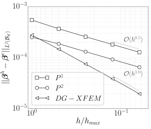
(a) Convergece in the $L^{2}(\mathcal{B}_{\mathscr{C}})$ norm

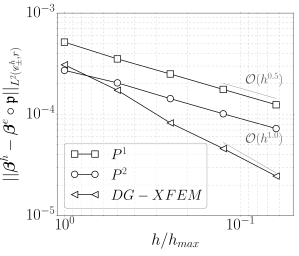
(b) Convergece in the $L^{2}(\mathscr{C}_{\pm}^{h},r)$ norm

Figure 10: Convergence of the solution.

Table 3: Convergence rates for stress intensity factors

	$P^{1}$				$P^{2}$				$DG-XFEM$
	$K_{I}$		$K_{II}$		$K_{I}$		$K_{II}$		$K_{I}$		$K_{II}$
$h_{\text{max}}/h$	Err.	$\mathcal{O}$	Err.	$\mathcal{O}$	Err.	$\mathcal{O}$	Err.	$\mathcal{O}$	Err.	$\mathcal{O}$	Err.	$\mathcal{O}$
1/1	5e-02	–	5e-02	–	4e-03	–	2e-02	–	5e-03	–	2e-02	–
1/2	2e-02	1.75	3e-02	0.82	5e-03	0.11	9e-03	1.24	9e-04	2.45	5e-03	1.99
1/4	8e-03	1.00	1e-02	1.03	2e-03	1.08	4e-03	1.06	3e-04	1.69	1e-03	1.91
1/8	4e-03	1.08	7e-03	1.02	9e-04	1.19	2e-03	0.94	1e-04	1.48	3e-04	1.91
1/16	2e-03	0.99	4e-03	1.03	5e-04	0.92	1e-03	0.92	2e-05	2.20	7e-05	2.23

(a) Traction free auxiliary fields ($\boldsymbol{\beta}^{\text{aux}}=\boldsymbol{\beta}^{\text{TF}}$) and tangential material variation ($\delta\boldsymbol{\gamma}=\delta\boldsymbol{\gamma}^{\text{TAN}}$).

[ Divergence-free ($\boldsymbol{\beta}^{\text{aux}}=\boldsymbol{\beta}^{\text{DFC}}$) and unidirectional material variation ($\delta\boldsymbol{\gamma}=\delta\boldsymbol{\gamma}^{\text{UNI}}$ ). ] $P^{1}$ $P^{2}$ $DG-XFEM$ $K_{I}$ $K_{II}$ $K_{I}$ $K_{II}$ $K_{I}$ $K_{II}$ $h_{\text{max}}/h$ Err. $\mathcal{O}$ Err. $\mathcal{O}$ Err. $\mathcal{O}$ Err. $\mathcal{O}$ Err. $\mathcal{O}$ Err. $\mathcal{O}$ 1/1 1e-02 – 3e-02 – 7e-03 – 1e-02 – 7e-03 – 1e-02 – 1/2 2e-03 2.54 2e-02 0.44 9e-04 2.93 5e-03 1.23 1e-03 2.59 1e-03 3.04 1/4 1e-03 0.91 9e-03 1.05 5e-04 0.92 2e-03 1.33 1e-04 3.37 2e-04 2.42 1/8 7e-04 0.76 5e-03 0.99 3e-04 0.78 1e-03 0.81 6e-05 0.92 8e-05 1.52 1/16 3e-04 0.99 2e-03 1.00 9e-05 1.57 5e-04 1.05 8e-06 2.77 3e-05 1.76 [ Divergence-free ($\boldsymbol{\beta}^{\text{aux}}=\boldsymbol{\beta}^{\text{DFC}}$) and tangential material variation ($\delta\boldsymbol{\gamma}=\delta\boldsymbol{\gamma}^{\text{TAN}}$ ).] $P^{1}$ $P^{2}$ $DG-XFEM$ $K_{I}$ $K_{II}$ $K_{I}$ $K_{II}$ $K_{I}$ $K_{II}$ $h_{\text{max}}/h$ Err. $\mathcal{O}$ Err. $\mathcal{O}$ Err. $\mathcal{O}$ Err. $\mathcal{O}$ Err. $\mathcal{O}$ Err. $\mathcal{O}$ 1/1 4e-02 – 1e-02 – 6e-03 – 7e-03 – 6e-03 – 8e-03 – 1/2 1e-02 1.74 1e-02 0.20 4e-03 0.56 3e-03 1.41 8e-04 2.85 2e-03 2.43 1/4 7e-03 1.00 5e-03 1.04 2e-03 1.06 1e-03 0.94 2e-04 2.09 4e-04 1.88 1/8 3e-03 1.08 3e-03 0.90 1e-03 0.82 6e-04 1.31 5e-05 2.11 9e-05 2.23 1/16 2e-03 0.97 1e-03 1.03 5e-04 1.13 2e-04 1.23 1e-05 2.07 2e-05 2.14

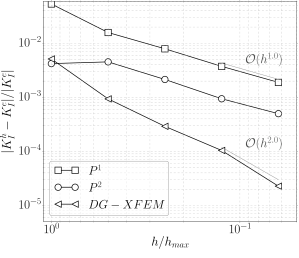
(a) $(\boldsymbol{\beta}^{\text{aux}},\delta\boldsymbol{\gamma})=(\boldsymbol{\beta}^{\text{TF}}_{\text{I}},\delta\boldsymbol{\gamma}^{\text{TAN}})$ .

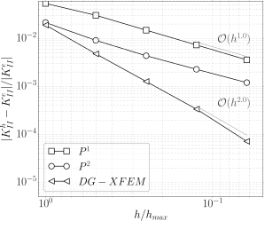
(b) $(\boldsymbol{\beta}^{\text{aux}},\delta\boldsymbol{\gamma})=(\boldsymbol{\beta}^{\text{TF}}_{\text{II}},\delta\boldsymbol{\gamma}^{\text{TAN}})$.

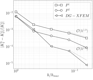
(c) $(\boldsymbol{\beta}^{\text{aux}},\delta\boldsymbol{\gamma})=(\boldsymbol{\beta}^{\text{DFC}}_{\text{I}},\delta\boldsymbol{\gamma}^{\text{UNI}})$.

(d) $(\boldsymbol{\beta}^{\text{aux}},\delta\boldsymbol{\gamma})=(\boldsymbol{\beta}^{\text{DFC}}_{\text{II}},\delta\boldsymbol{\gamma}^{\text{UNI}})$.

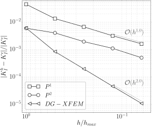
(e) $(\boldsymbol{\beta}^{\text{aux}},\delta\boldsymbol{\gamma})=(\boldsymbol{\beta}^{\text{DFC}}_{\text{I}},\delta\boldsymbol{\gamma}^{\text{TAN}})$.

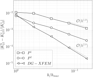
(f) $(\boldsymbol{\beta}^{\text{aux}},\delta\boldsymbol{\gamma})=(\boldsymbol{\beta}^{\text{DFC}}_{\text{II}},\delta\boldsymbol{\gamma}^{\text{TAN}})$.

Figure 11: Convergence of the stress intensity factors for the circular arc crack

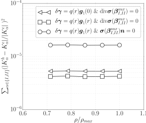
Figure 12: Contour independence of the interaction integral

5.3 Power Function Crack

The second example we consider is the one of the power function crack $\mathscr{C}=\{(x,x^{3})|\,x\in[0,1]\}$ loaded by a force field ${\boldsymbol{b}}$ and crack face traction $\overline{\boldsymbol{t}}$, see Fig. 13.

The exact stress field is constructed by a superposition of a singular stress field $\hat{\boldsymbol{\sigma}}^{e}$ with a bounded field $\boldsymbol{\sigma}_{{\boldsymbol{b}}}$ as

$$\boldsymbol{\sigma}^{e}=\hat{\boldsymbol{\sigma}}^{e}+\boldsymbol{\sigma}_{{\boldsymbol{b}}}.$$

The field $\hat{\boldsymbol{\sigma}}^{e}$ is constructed as

$$\hat{\boldsymbol{\sigma}}^{e}={\left(\sigma^{I}_{ij}+\sigma^{II}_{ij}\right)}{\boldsymbol{g}}_{i}(0)\otimes{\boldsymbol{g}}_{j}(0),$$

where $\sigma_{ij}^{I,II}$ are given in §A and are evaluated for values of $\vartheta\in[-\pi-\zeta(r),\pi-\zeta(r)]$, as discussed in §2.2. The bounded stress field $\boldsymbol{\sigma}_{{\boldsymbol{b}}}$ is constructed as

$$\boldsymbol{\sigma}_{\boldsymbol{b}}=x{\boldsymbol{e}}_{x}\otimes{\boldsymbol{e}}_{x}+y{\boldsymbol{e}}_{y}\otimes{\boldsymbol{e}}_{y}.$$

Note that

$$\nabla\cdot\boldsymbol{\sigma}^{e}=\nabla\cdot\hat{\boldsymbol{\sigma}}^{e}+\nabla\cdot\boldsymbol{\sigma}_{{\boldsymbol{b}}}=\nabla\cdot\boldsymbol{\sigma}_{{\boldsymbol{b}}}=-{\boldsymbol{b}},$$

where

$${\boldsymbol{b}}=-({\boldsymbol{e}}_{x}+{\boldsymbol{e}}_{y}).$$

It is worth remarking that the stress intensity factors of $\boldsymbol{\sigma}^{e}$ will correspond to those of the singular field $\hat{\boldsymbol{\sigma}}^{e}$ without any perturbation from the bounded field. In fact, given that both $\lim_{r\to 0}\sqrt{r}\hat{\boldsymbol{\sigma}}^{e},\lim_{r\to 0}\sqrt{r}\boldsymbol{\sigma}_{{\boldsymbol{b}}}={\bf 0}$ exist, we have

$$\lim_{r\to 0}\sqrt{r}\boldsymbol{\sigma}^{e}=\lim_{r\to 0}\sqrt{r}(\hat{\boldsymbol{\sigma}}^{e}+\boldsymbol{\sigma}_{{\boldsymbol{b}}})=\lim_{r\to 0}\sqrt{r}\boldsymbol{\sigma}_{I,II}+\lim_{r\to 0}\sqrt{r}\boldsymbol{\sigma}_{{\boldsymbol{b}}}=\lim_{r\to 0}\sqrt{r}\boldsymbol{\sigma}_{I,II}.$$

For our example we take the stress intensity factors of $\hat{\boldsymbol{\sigma}}^{e}$ to be $K^{e}_{I}=K^{e}_{II}=1$.

Figures 13 and 14 show the schematic of the problem and the modeled domain with the applied boundary conditions, respectively. For the simulations the modeled domain was given by $\mathcal{B}=[0,2]\times[-0.25,1.75]$.

Like for the previous example, we computed the solution for several levels of refinement and investigated the convergence of the computed stress intensity factors.

The error measures (42) and (43) were observed to decrease as $\mathcal{O}(h^{1/2})$ and $\mathcal{O}(h)$ for the first- and second-order methods, respectively. The values are plotted in Fig. 15 and the errors and the computed rates of convergence are tabulated in Table 5.3.

The stress intensity factors were observed to converge to the analytical value as $\mathcal{O}(h)$ and $\mathcal{O}(h^{2})$ when using the solution of the first- and second-order methods, respectively. The values of the error in the stress intensity factors are plotted in Fig. 5.2, and the errors, as well as the computed convergence rates, are provided in Table 5.2.

Lastly, in Fig. 17 we illustrate the independence of the interaction integral on the size of the support of $\delta\boldsymbol{\gamma}$ by plotting the stress intensity factors for five values of $\rho/\rho_{\text{max}}$ ranging from $\sim 0.7$ to $1$, for $\rho_{\text{max}}=0.5$.

Figure 13: The power function crack problem

Figure 14: Modeled subdomain

Table 4: Convergence rates of the derivatives of the solution for the circular arc crack problem

(a) Domain convergence

[Trace convergence] $\|\boldsymbol{\beta}^{h}-\boldsymbol{\beta}^{e}\circ\mathfrak{p}\|_{L^{2}(\mathscr{C}^{h}_{\pm},r)}$ $P^{1}$ $P^{2}$ $DG-XFEM$ $h_{\text{max}}/h$ Err. $\mathcal{O}$ Err. $\mathcal{O}$ Err. $\mathcal{O}$ 1 0.00066 – 0.00037 – 0.00035 – 2 0.00050 0.40 0.00029 0.34 0.00013 1.39 4 0.00036 0.48 0.00021 0.48 0.00006 1.06 8 0.00026 0.43 0.00015 0.48 0.00003 0.97 16 0.00019 0.49 0.00011 0.50 0.00002 0.99

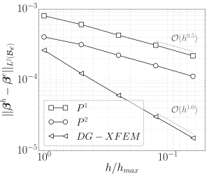
(a) Convergence in the $L^{2}(\mathcal{B}_{\mathscr{C}})$ norm

(b) Convergence in the $L^{2}(\mathscr{C}_{\pm}^{h},r)$ norm

Figure 15: Convergence of the solution.

Table 5: Convergence rates for stress intensity factors

(a) Traction free auxiliary fields ($\boldsymbol{\beta}^{\text{aux}}=\boldsymbol{\beta}^{\text{TF}}$) and tangential material variation ($\delta\boldsymbol{\gamma}=\delta\boldsymbol{\gamma}^{\text{TAN}}$).

[ Divergence-free ($\boldsymbol{\beta}^{\text{aux}}=\boldsymbol{\beta}^{\text{DFC}}$) and unidirectional material variation ($\delta\boldsymbol{\gamma}=\delta\boldsymbol{\gamma}^{\text{UNI}}$ ). ] $P^{1}$ $P^{2}$ $DG-XFEM$ $K_{I}$ $K_{II}$ $K_{I}$ $K_{II}$ $K_{I}$ $K_{II}$ $h_{\text{max}}/h$ Err. $\mathcal{O}$ Err. $\mathcal{O}$ Err. $\mathcal{O}$ Err. $\mathcal{O}$ Err. $\mathcal{O}$ Err. $\mathcal{O}$ 1/1 1e-01 – 4e-02 – 3e-02 – 4e-03 – 1e-02 – 7e-03 – 1/2 7e-02 0.72 2e-02 0.81 2e-02 0.70 5e-03 0.37 3e-03 1.86 1e-03 2.36 1/4 3e-02 0.99 1e-02 1.02 1e-02 0.99 3e-03 0.87 7e-04 2.00 3e-04 2.35 1/8 2e-02 0.94 6e-03 0.91 5e-03 0.96 2e-03 0.72 2e-04 1.97 4e-05 2.68 1/16 9e-03 0.98 3e-03 0.99 3e-03 1.04 9e-04 1.05 6e-05 1.70 7e-06 2.58 [ Divergence-free ($\boldsymbol{\beta}^{\text{aux}}=\boldsymbol{\beta}^{\text{DFC}}$) and tangential material variation ($\delta\boldsymbol{\gamma}=\delta\boldsymbol{\gamma}^{\text{TAN}}$ ).] $P^{1}$ $P^{2}$ $DG-XFEM$ $K_{I}$ $K_{II}$ $K_{I}$ $K_{II}$ $K_{I}$ $K_{II}$ $h_{\text{max}}/h$ Err. $\mathcal{O}$ Err. $\mathcal{O}$ Err. $\mathcal{O}$ Err. $\mathcal{O}$ Err. $\mathcal{O}$ Err. $\mathcal{O}$ 1/1 1e-01 – 4e-02 – 3e-02 – 4e-03 – 1e-02 – 7e-03 – 1/2 6e-02 0.72 2e-02 0.83 2e-02 0.70 5e-03 0.47 3e-03 1.88 2e-03 2.28 1/4 3e-02 0.99 1e-02 1.02 1e-02 1.00 3e-03 0.90 8e-04 1.98 3e-04 2.32 1/8 2e-02 0.94 6e-03 0.91 5e-03 0.95 2e-03 0.69 2e-04 1.94 5e-05 2.71 1/16 9e-03 0.98 3e-03 0.99 3e-03 1.04 8e-04 1.05 6e-05 1.68 1e-05 2.05

(a) $(\boldsymbol{\beta}^{\text{aux}},\delta\boldsymbol{\gamma})=(\boldsymbol{\beta}^{\text{TF}}_{\text{I}},\delta\boldsymbol{\gamma}^{\text{TAN}})$ .

(b) $(\boldsymbol{\beta}^{\text{aux}},\delta\boldsymbol{\gamma})=(\boldsymbol{\beta}^{\text{TF}}_{\text{II}},\delta\boldsymbol{\gamma}^{\text{TAN}})$.

(c) $(\boldsymbol{\beta}^{\text{aux}},\delta\boldsymbol{\gamma})=(\boldsymbol{\beta}^{\text{DFC}}_{\text{I}},\delta\boldsymbol{\gamma}^{\text{UNI}})$.

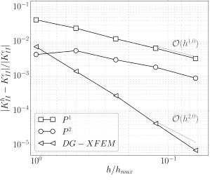
(d) $(\boldsymbol{\beta}^{\text{aux}},\delta\boldsymbol{\gamma})=(\boldsymbol{\beta}^{\text{DFC}}_{\text{II}},\delta\boldsymbol{\gamma}^{\text{UNI}})$.

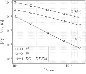
(e) $(\boldsymbol{\beta}^{\text{aux}},\delta\boldsymbol{\gamma})=(\boldsymbol{\beta}^{\text{DFC}}_{\text{I}},\delta\boldsymbol{\gamma}^{\text{TAN}})$.

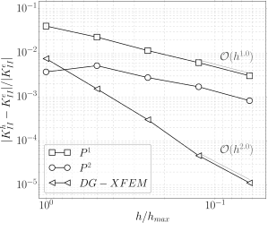
(f) $(\boldsymbol{\beta}^{\text{aux}},\delta\boldsymbol{\gamma})=(\boldsymbol{\beta}^{\text{DFC}}_{\text{II}},\delta\boldsymbol{\gamma}^{\text{TAN}})$.

Figure 16: Convergence of the stress intensity factors for the power function crack problem

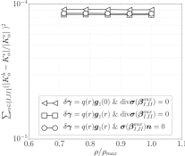
Figure 17: Contour independence of the interaction integral

Appendix A Modes I and II Asymptotic Solutions

We recall below the components of displacement, gradient of displacements and the stress fields for a straight crack lying on the axis $\vartheta=\pm\pi,r\in[0,\infty)$ as derived in [14]. The components are given for a set of right-handed orthonormal basis with the $1$ axis aligned with the crack.

For $\kappa=3-4\nu$ for plane strain and $\kappa=(3-4\nu)/(1+\nu)$ for plane stress, the displacements are given by

$$u^{I}_{1} =\sqrt{\frac{r}{2\pi}}\frac{1}{2\mu}\cos\left(\frac{\vartheta}{2}\right)(\kappa-\cos(\vartheta)),$$

$$u^{I}_{2} =\sqrt{\frac{r}{2\pi}}\frac{1}{2\mu}\sin\left(\frac{\vartheta}{2}\right)(\kappa-\cos(\vartheta));$$

$$u^{II}_{1} =\sqrt{\frac{r}{2\pi}}\frac{1}{2\mu}\sin\left(\frac{\vartheta}{2}\right)(2+\kappa+\cos(\vartheta)),$$

$$u^{II}_{2} =\sqrt{\frac{r}{2\pi}}\frac{1}{2\mu}\cos\left(\frac{\vartheta}{2}\right)(2-\kappa-\cos(\vartheta)).$$

The gradient of displacements are given by

$$\nabla u_{11}^{I}(r,\vartheta) =\dfrac{1}{4\mu\sqrt{2\pi r}}\cos\left(\dfrac{\vartheta}{2}\right)(-\cos(\vartheta)+\cos(2\vartheta)+\kappa-1),$$

$$\nabla u_{12}^{I}(r,\vartheta) =\dfrac{1}{4\mu\sqrt{2\pi r}}\sin\left(\dfrac{\vartheta}{2}\right)(\cos(\vartheta)+\cos(2\vartheta)+\kappa+1),$$

$$\nabla u_{21}^{I}(r,\vartheta) =\dfrac{1}{4\mu\sqrt{2\pi r}}\sin\left(\dfrac{\vartheta}{2}\right)(\cos(\vartheta)+\cos(2\vartheta)-\kappa-1),$$

$$\nabla u_{22}^{I}(r,\vartheta) =\dfrac{1}{4\mu\sqrt{2\pi r}}\cos\left(\dfrac{\vartheta}{2}\right)(\cos(\vartheta)-\cos(2\vartheta)+\kappa-1),$$

$$\nabla u_{11}^{II}(r,\vartheta) =-\dfrac{1}{4\mu\sqrt{2\pi r}}\sin\left(\frac{\vartheta}{2}\right)(\cos(\vartheta)+\cos(2\vartheta)+\kappa+1),$$

$$\nabla u_{12}^{II}(r,\vartheta) =\dfrac{1}{4\mu\sqrt{2\pi r}}\cos\left(\frac{\vartheta}{2}\right)(-\cos(\vartheta)+\cos(2\vartheta)+\kappa+3),$$

$$\nabla u_{21}^{II}(r,\vartheta) =\dfrac{1}{4\mu\sqrt{2\pi r}}\cos\left(\frac{\vartheta}{2}\right)(-\cos(\vartheta)+\cos(2\vartheta)-\kappa+1),$$

$$\nabla u_{22}^{II}(r,\vartheta) =\dfrac{1}{4\mu\sqrt{2\pi r}}\sin\left(\frac{\vartheta}{2}\right)(\cos(\vartheta)+\cos(2\vartheta)-\kappa+3).$$

Lastly the stress components are given by

$$\sigma_{11}^{I}(r,\vartheta) =\frac{1}{\sqrt{2\pi r}}\left[1-\sin\left(\frac{\vartheta}{2}\right)\sin\left(\frac{3\vartheta}{2}\right)\right]\cos\left(\frac{\vartheta}{2}\right),$$

$$\sigma_{22}^{I}(r,\vartheta) =\frac{1}{\sqrt{2\pi r}}\left[\sin\left(\frac{\vartheta}{2}\right)\sin\left(\frac{3\vartheta}{2}\right)+1\right]\cos\left(\frac{\vartheta}{2}\right),$$

$$\sigma_{12}^{I}(r,\vartheta) =\frac{1}{\sqrt{2\pi r}}\sin\left(\frac{\vartheta}{2}\right)\cos\left(\frac{\vartheta}{2}\right)\cos\left(\frac{3\vartheta}{2}\right),$$

$$\sigma_{11}^{II}(r,\vartheta) =-\frac{1}{\sqrt{2\pi r}}\sin\left(\frac{\vartheta}{2}\right)\left[\cos\left(\frac{\vartheta}{2}\right)\cos\left(\frac{3\vartheta}{2}\right)+2\right],$$

$$\sigma_{22}^{II}(r,\vartheta) =\frac{1}{\sqrt{2\pi r}}\left[1-\sin\left(\frac{\vartheta}{2}\right)\sin\left(\frac{3\vartheta}{2}\right)\right]\cos\left(\frac{\vartheta}{2}\right),$$

$$\sigma_{12}^{II}(r,\vartheta) =\frac{1}{\sqrt{2\pi r}}\sin\left(\frac{\vartheta}{2}\right)\cos\left(\frac{\vartheta}{2}\right)\cos\left(\frac{3\vartheta}{2}\right).$$

Note that the above fields satisfy

$$K_{I}[\nabla{\boldsymbol{u}}^{I}]=1, K_{II}[\nabla{\boldsymbol{u}}^{I}]=0,$$

$$K_{I}[\nabla{\boldsymbol{u}}^{II}]=0, K_{II}[\nabla{\boldsymbol{u}}^{II}]=1.$$

Appendix B Convergence of a continuous affine functional

In this appendix we first state and prove a proposition about the convergence of linear and continuous functionals of a convergent family of solutions. This proof is essentially adapted from similar results in [33, 32]. We next apply this result to the interaction integral functional (37).

Proposition.

Let $V$ be a Hilbert space and $V^{h}\subset V$ be its finite dimensional approximation. Let $a:V\times V\to\mathbb{R}$ be a bilinear, continuous and coercive form with $a(u,v)\leq C_{1}\|u\|_{V}\|v\|_{V}$ for all $u,v\in V$. Let $F:V\to\mathbb{R}$ be linear and continuous functional, and let $G:V\to\mathbb{R}$ be an affine and continuous functional. Take $u$ to be the solution to $a(u,v)=F(v),\,\forall v\in V$ and $u^{h}$ the solution to $a(u^{h},v^{h})=F(v^{h}),\,\forall v^{h}\in V^{h}$. Let $w\in V$ be the unique member of $V$ such that $a(v,w)=G(v)-G(0),\,\forall v\in V$. We further assume that there exist positive real numbers $C_{2}$ and $C_{3}$ independent of $h$ such that $\|u-u^{h}\|_{V}\leq C_{2}h^{k}$ and $\inf_{w^{h}\in V^{h}}\|w-w^{h}\|_{V}\leq C_{3}h^{k}$. Then there exists $C$ independent of $h$ such that

$$\left|G(u)-G\left(u^{h}\right)\right|\leq Ch^{2k}.$$

Proof.

From the definition of $w$,

$$G(u)-G\left(u^{h}\right)=a\left(u-u^{h},w\right).$$

Furthermore note that for any $w^{h}\in V^{h}$,

$$a\left(u-u^{h},w\right)=a\left(u-u^{h},w-w^{h}\right)+a\left(u-u^{h},w^{h}\right)=a\left(u-u^{h},w-w^{h}\right),$$

where we have taken advantage of Galerkin orthogonality, i.e.,

$$a\left(u-u^{h},w^{h}\right)=a\left(u,w^{h}\right)-a\left(u^{h},w^{h}\right)=F\left(w^{h}\right)-F\left(w^{h}\right)=0.$$

Therefore we have

$$\left|G(u)-G\left(u^{h}\right)\right|=\left|a\left(u-u^{h},w-w^{h}\right)\right|\leq C_{1}\left\|u-u^{h}\right\|_{V}\left\|w-w^{h}\right\|_{V}.$$

Since $w^{h}$ is arbitrary, we have

$$\left|G(u)-G\left(u^{h}\right)\right|\leq C_{1}\left\|u-u^{h}\right\|_{V}\inf_{w^{h}\in V^{h}}\left\|w-w^{h}\right\|_{V}\leq C_{1}C_{2}C_{3}h^{2k}.$$

Taking $C=C_{1}C_{2}C_{3}$ yields the conclusion. ∎

The application of this proposition to the interaction integral functionals here requires some additional work to account for the difference between domains in curvilinear cracks, and the use of quadrature rules. However, disregarding these differences, and assuming that $\mathcal{B}^{h}_{\mathscr{C}}=\mathcal{B}_{\mathscr{C}}$ and that exact quadrature is adopted, we have $\mathcal{I}^{h}=\mathcal{I}$, and for the standard finite element method in §5.1, $\mathcal{V}^{h}\subset H^{1}(\mathcal{B}_{\mathscr{C}};\mathbb{R}^{2})$, $\forall h$. Now, in its first argument, $\mathcal{I}[\boldsymbol{\beta},\boldsymbol{\beta}^{\text{TF}},\delta\boldsymbol{\gamma}^{\text{TAN}}]$ is affine and continuous in $L^{2}(\mathcal{B}_{\mathscr{C}};\mathbb{R}^{2\times 2})$, so we set $G({\boldsymbol{u}})=\mathcal{I}[\nabla{\boldsymbol{u}},\boldsymbol{\beta}^{\text{TF}},\delta\boldsymbol{\gamma}^{\text{TAN}}]$ (c.f. (37)) and can use the above proposition. Since for the standard finite element method it is known that there exists $C>0$ independent of $h$ such that $\|{\boldsymbol{u}}-{\boldsymbol{u}}^{h}\|_{H^{1}(\mathcal{B}_{\mathscr{C}};\mathbb{R}^{2})}\leq Ch^{k}$, $\forall h$, then

$$\left|G({\boldsymbol{u}})-G\left({\boldsymbol{u}}^{h}\right)\right|\leq\overline{C}h^{2k}$$

for some $\overline{C}\in\mathbb{R}^{+}$.

This proposition is not directly applicable to the discontinuous Galerkin method in §5.1, because in this case it is also necessary to account for the use of an approximation space that does not conform to $H^{1}$. Finally, the two functionals $G({\boldsymbol{u}})=\mathcal{I}[\nabla{\boldsymbol{u}},\boldsymbol{\beta}^{\text{DFC}},\delta\boldsymbol{\gamma}]$ in (35) and (36) are not continuous in $H^{1}(\mathcal{B}_{\mathscr{C}};\mathbb{R}^{2})$, because of the evaluations of $\nabla{\boldsymbol{u}}$ on the crack faces, so we cannot directly apply the above result.

References

- [1] Liu XY, Xiao QZ, Karihaloo BL. XFEM for direct evaluation of mixed mode SIFs in homogeneous and bi-materials. International Journal for Numerical Methods in Engineering 2004; 59(8):1103–1118.
- [2] Shen Y, Lew A. An optimally convergent discontinuous-Galerkin-based extended finite element method for fracture mechanics. International Journal for Numerical Methods in Engineering 2010; 82(6):716–755.
- [3] Chiaramonte MM, Shen Y, Lew AJ. The h-version of the method of auxiliary mapping for higher order solutions of crack and re-entrant corner problems 2014. In preparation.
- [4] Rice JR. A path independent integral and the approximate analysis of strain concentration by notches and cracks. Journal of Applied Mechanics 1968; 35:379–386.
- [5] Stern M, Becker EB, Dunham RS. A contour integral computation of mixed mode stress intensity factors. International Journal of Fracture 1976; 69:359–368.
- [6] Eshelby JD. The force on an elastic singularity. Philosophical Transactions of the Royal Society London 1951; 244:87–112.
- [7] Freund LB. Stress intensity factor calculations based on a conservation integral. International of Journal of Solids and Structures 1978; 14:241–250.
- [8] Shih CF, Moran B, Nakamura T. Energy release rate along a three-dimensional crack front in a thermally stressed body. International Journal of Fracture 1986; .
- [9] Moran B, Shih CF. Crack tip and associated domain integrals from momentum and energy balance. Engineering Fracture Mechanics 1987; 27(6):615–642.
- [10] Moran B, Shih CF. A general treatment of crack tip contour integrals. International Journal of Fracture 1987; 35:295–310.
- [11] Irwin GR. Analysis of stresses and strains near the end of a crack traversing a plate. J. Appl. Mech. 1957; 24:361–364.
- [12] Chang J, Wu D. Stress intensity factor computation along a non-planar curved crack in three dimensions. International Journal of Solids and Structures 2007; 44(2):371–386.
- [13] Williams ML. Stress singularities resulting from various boundary conditions in angular corners of plate in extension. Journal of Applied Mechanics 1952; 19:526–528.
- [14] Williams ML. On the stress distribution at the base of a stationary crack. Journal of Applied Mechanics 1957; 24:109–158.
- [15] Yau JF, Wang SS, Corten HT. A mixed-mode crack analysis of isotropic solids using conservation laws of elasticity. Journal of Applied Mechanics 1980; 47:335–341.
- [16] Nakamura T, Parks DM. Antisymmetrical 3-D stress field near the crack front of a thin elastic plate. International Journal of Solids and Structures 1989; 25(12):1411–1426.
- [17] Nakamura T. Three-dimensional stress fields of elastic interface cracks. Journal of Applied Mechanics 1991; 58(4):939–946.
- [18] Nahta R, Moran B. Domain integrals for axisymmetric interface crack problems. International Journal of Solids and Structures 1993; 30(15):2027–2040.
- [19] Gosz M, Dolbow J, Moran B. Domain integral formulation for stress intensity factor computation along curved three-dimensional interface cracks. International Journal of Solids and Structures 1998; 15:1763–1783.
- [20] Kim YJ, Kim HG, Im S. Mode decomposition of three-dimensional mixed-mode cracks via two-state integrals. International Journal of Solids and Structures 2001; 38(36–37):6405–6426.
- [21] Daimon R, Okada H. Mixed-mode stress intensity factor evaluation by interaction integral method for quadratic tetrahedral finite element with correction terms. Engineering Fracture Mechanics 2014; 115:22–42.
- [22] Walters MC, Paulino GH, Dodds RH Jr. Interaction integral procedures for 3-D curved cracks including surface tractions. Engineering Fracture Mechanics 2005; 72(11):1635–1663.
- [23] Gosz M, Moran B. An interaction energy integral method for computation of mixed-mode stress intensity factors along non-planar crack fronts in three dimensions. Engineering Fracture Mechanics 2002; 69(3):299–319.
- [24] Sukumar N, Chopp DL, Béchet E, Moës N. Three-dimensional non-planar crack growth by a coupled extended finite element and fast marching method. International Journal for Numerical Methods in Engineering 2008; 76(5):727–748.
- [25] Moës N, Gravouil A, Belytschko T. Non-planar 3D crack growth by the extended finite element and level sets–Part I: Mechanical model. International Journal for Numerical Methods in Engineering 2002; 53(11):2549–2568.
- [26] González-Albuixech VF, Giner E, Tarancón JE, Fuenmayor FJ, Gravouil A. Domain integral formulation for 3-D curved and non-planar cracks with the extended finite element method. Computer Methods in Applied Mechanics and Engineering 2013; 264:129–144.
- [27] González-Albuixech VF, Giner E, Tarancón JE, Fuenmayor FJ, Gravouil A. Convergence of domain integrals for stress intensity factor extraction in 2-D curved cracks problems with the extended finite element method. Int. J. Numer. Meth. Engng. 2013; 94:740 –757.
- [28] Moghaddam AS, Ghajar R, Alfano M. Finite element evaluation of stress intensity factors in curved non-planar cracks in FGMs. Mechanics Research Communications 2011; 38(1):17–23.
- [29] Ghajar R, Moghaddam AS, Alfano M. An improved numerical method for computation of stress intensity factors along 3D curved non-planar cracks in FGMs. International Journal of Solids and Structures 2011; 48(1):208–216.
- [30] Griffith AA. The phenomena of rupture and flow in solids. Philosophical Transactions of the Royal Society of London 1921; 221:163–198.
- [31] Eshelby JD. The elastic energy-momentum tensor. Journal of Elasticity 1975; 5:321–335.
- [32] Guillaume P, Masmoudi M. Computation of high order derivatives in optimal shape design. Numerische Mathematik 1994; 67(2):231–250.
- [33] Buscaglia G, Jai M. Sensitivity analysis and taylor expansions in numerical homogenization problems. Numerische Mathematik 2000; 85(1):49–75.
- [34] Muskhelishvili NI ( (ed.)). Some Basic Problems of the Mathematical Theory of Elasticity: Fundamental Equations, Plane Theory of Elasticity, Torsion, and Bending (translated from Russian). 2nd edn., Noordhoff International Publishing: Leyden, The Netherlands, 1977.
- [35] Rangarajan R, Chiaramonte MM, Hunsweck MJ, Shen Y, Lew AJ. Simulating curvilinear crack propagation in two dimensions with universal meshes. International Journal for Numerical Methods in Engineering 2014; 10.1002/nme.4731.
- [36] Cotterell B, Rice JR. Slightly curved or kinked cracks. Int. J. of Fracture Mech. 1965; 16:155–168.