FRACTIONALLY INTEGRATED COGARCH PROCESSES

STEPHAN HAUG, CLAUDIA KLÜPPELBERG AND GERMAN STRAUB

Technical University of Munich

Abstract: We construct fractionally integrated continuous-time GARCH models, which capture the observed long range dependence of squared volatility in high-frequency data. Since the usual Molchan-Golosov and Mandelbrot-van-Ness fractional kernels lead to problems in the definition of the model, we resort to moderately long memory processes by choosing a fractional parameter $d\in(-0.5,0)$ and remove the singularities of the kernel to obtain non-pathological sample paths. The volatility of the new fractional COGARCH process has positive features like stationarity, and its covariance function shows an algebraic decay, which make it applicable to econometric high-frequency data. In an empirical application the model is fitted to exchange rate data using a simulation-based version of the generalised method of moments.

Key words and phrases: fractionally integrated COGARCH, FICOGARCH, long range dependence, fractional subordinator, stationarity, Lévy process, stochastic volatility modelling

1 Introduction

Long range dependence in time series or their latent volatilities has been observed in many application areas and is often modelled by fractional processes. From a statistical point of view, using long range dependence models for data or their latent structure, the question should be asked, where this effect originates from. Obviously, a small deterministic trend or seasonality introduces long range dependence into the data. But also, as is well-known (cf. Mikosch and Starica (2004), Lai and Xing (2006) and Davis and Yau (2011)), change points in the model or a change of parameters in time can be responsible for long range dependence effects. On the other hand, when these effects are small, and trends or parameters change very slowly in time, they are statistically often not detectable; cf. Dette et al. (2017) for test procedures and a literature review on this topic. This is in particular true, when such small effects occur in the volatility process, which is latent. Consequently, a long range dependent model may well be the best choice as it at least captures the observed behaviour.

Prominent discrete-time models in finance have been early on discussed for instance in Baillie (1996), Baillie, Bollerslev, and Mikkelsen (1996), Bollerslev and Mikkelsen (1996), Ding, Granger, and Engle (1993) and Geweke and Porter-Hudak (1983).

When it comes to continuous-time stochastic volatility processes long memory Gaussian models for the log-volatility have been suggested and analysed in Comte (1996), Comte and Renault (1996), and Comte and Renault (1998). As Gaussian models are distributionally restricted, such concepts have been extended to more general models in two ways. Comte, Coutin, and Renault (2012) introduce long memory in the Heston model by considering an affine volatility model, where they fractionally integrate the square-root volatility process. As they emphasize, there is nowadays a quite general agreement on the idea that jump components in the return process (and possibly in the volatility process itself) are needed to explain very short term option prices, but long memory processes can address option pricing puzzles as steep volatility smiles in long term options and co-movements between implied and realized volatility for longer maturities without introducing unrealistic volatility behavior in both short and long term returns (cf. Comte et al. (2012) for more extensive discussions).

Another line of research involves general Lévy processes instead of Brownian motion. For instance, Anh, Heyde, and Leonenko (2002) proposed a Lévy driven stochastic volatility model, where the volatility process is of moving average type and allows for long memory by the choice of the moving average kernel. Another related approach replaces the fractional Brownian motion driving process by a fractional Lévy process, which have been introduced as analogues to fractional Brownian motion in Marquardt (2006b). This leads to fractional Ornstein-Uhlenbeck processes and other continuous-time long memory models as in Fink and Klüppelberg (2011).

Introducing long range dependence in non-linear models like ARCH and GARCH and their continuous-time counterparts resulting in stationary models is much more difficult, and we discuss this first for discrete-time models. Different approaches have been proposed in the literature for defining long range dependent ARCH and GARCH models. Baillie et al. (1996) and Ding and Granger (1996) were among the first to have discussed ways to incorporate long memory in a stationary ARCH model. But some of these approaches have certain drawbacks as emphasised in Mikosch and Starica (2003). Indeed, Douc, Roueff, and Soulier (2008) were the first to specify conditions for the existence of a strictly stationary solution to the fractionally integrated GARCH$(p,d,q)$ equation. But they give a proof only for the case $p=q=0$ and certain values of $d\in(d^{\ast},1)$ for $d^{\ast}>0$, where they use the fact that fractionally integrated GARCH$(0,d,0)$ models are a subclass of ARCH($\infty$) models. The conditions derived in Kazakevičius and Leipus (2003) for the existence of a strictly stationary solution of an ARCH($\infty$) model rule out the fractionally integrated GARCH model. The model was extended by Douc et al. (2008), however, the second moment of the resulting stationary solution is not finite. Giraitis, Surgailis, and Škarnulis (2015) showed the existence of a stationary FIGARCH process with finite variance by considering it as solution of an ARCH($\infty$) representation without constant term in the defining equation. They also proved that the volatility process in this model has a covariance function which is non-summable and, hence, possesses a long memory property.

The goal of this paper is to construct a fractionally integrated continuous-time GARCH model in order to capture long range dependence of squared volatility as observed in high-frequency data. Our approach to obtain a new continuous-time non-linear stochastic volatility model is based on the continuous-time GARCH (COGARCH) process. The definition of the COGARCH process has been based on replacing the driving noise of a GARCH model by the jumps of a Lévy process. In order to define a fractionally integrated COGARCH process, we cannot use the fractionally integrated GARCH model as a sole guidance because of the problems discussed above. However, it will be helpful to review the main ideas of the construction of the COGARCH process before defining a new fractionally integrated version.

1.1 Review of continuous-time GARCH models

The GARCH(1,1) model is a discrete-time process with three parameters, $a_{0}>0$, $a_{1}\geq 0$, $b_{1}\geq 0$, specifying the variance as a discrete-time stochastic recursion, or difference equation. We write it using two equations, one specifying the mean level process (the observed data, perhaps after removal of trend or other deterministic feature, to approximate stationarity) and the other specifying the variance process, which is time dependent and randomly fluctuating. Thus,

$$Y_{i}=\varepsilon_{i}\sigma_{i}\,,\quad i=1,2,\ldots\,,$$ (1.1)

with squared volatility

$$\sigma^{2}_{i}=a_{0}+a_{1}Y_{i-1}^{2}+b_{1}\sigma^{2}_{i-1}=a_{0}+(a_{1}\varepsilon_{i-1}^{2}+b_{1})\sigma^{2}_{i-1}\,,\quad i=1,2,\ldots\,.$$ (1.2)

Here the starting values $\varepsilon_{0}$ and $\sigma_{0}$ are given quantities, possibly random, and usually assumed independent of $(\varepsilon_{i})_{i=1,2,\ldots}$, which are the sole source of randomness in the model. The $\varepsilon_{i}$, $i=1,2,\ldots$, are assumed to be independent identically distributed (i.i.d.) random variables with mean 0. Serial dependence between the $Y_{i}$ is introduced via the dependence of the $\sigma^{2}_{i}$ on their past values. Conditional on $\sigma_{i}$, $Y_{i}$ simply has the distribution of $\varepsilon_{i}$, scaled by $\sigma_{i}$, which in general (as long as $a_{1},b_{1}>0$) is time dependent, hence the conditional heteroscedasticity part of the terminology. The “autoregressive" aspect refers to the form of the dependence of $\sigma^{2}_{i}$ on $\sigma^{2}_{i-1}$.

1.1.1 Continuous-time limits of GARCH models

Motivated by the availability of high-frequency data and by a need for option pricing technologies for realistic models, classical diffusion limits have been used in a natural way to obtain continuous-time limits of discrete-time processes. For the GARCH(1,1) model, the best-known limit model is the volatility-modulated model due to Nelson (1990) given by

$$\mathrm{d}G_{t}=\sigma_{t}{\rm d}B_{t}^{(1)},\qquad t\geq 0,$$

where the squared volatility process $(\sigma^{2}_{t})_{t\geq 0}$ is the solution of the stochastic differential equation (SDE)

$$\mathrm{d}\sigma^{2}_{t}=\left(\alpha_{0}-\beta_{1}\sigma^{2}_{t}\right)\mathrm{d}t+\alpha_{1}\sigma^{2}_{t}\mathrm{d}B_{t}^{(2)},\qquad t>0,$$

with initial values $G_{0}$ and ${\sigma}_{0}^{2}$, $B^{(1)}$ and $B^{(2)}$ are independent Brownian motions, and parameters $\alpha_{0}>0$, $\alpha_{1}\geq 0,\beta_{1}\geq 0$.

Unfortunately, diffusion limits can lose certain essential properties of the discrete-time models. It is surprising and counter-intuitive, for example, that Nelson’s diffusion limit of the GARCH process is driven by two independent Brownian motions, i.e., has two independent sources of randomness, whereas the discrete-time GARCH process is driven only by a single i.i.d. noise sequence. One of the features of the GARCH process is the idea that large innovations in the price process are almost immediately manifested as innovations in the volatility process, but this feedback mechanism is lost in models such as Nelson’s continuous-time version. Further, the appearance of an extra source of variation can have implications for completeness of the model when used for option pricing.

The phenomenon that a diffusion limit may be driven by two independent Brownian motions, while the discrete-time model is given in terms of a single i.i.d. sequence, is not restricted to the classical GARCH process. Duan (1997) has shown that this occurs for many GARCH like processes.

Moreover, such continuous-time limits can have distinctly different statistical properties compared to the original discrete-time processes. As was shown in Wang (2002), parameter estimation in the discrete-time GARCH and the corresponding continuous-time limit stochastic volatility model may yield different estimates. Thus these kinds of continuous-time models are probabilistically and statistically different from their discrete-time progenitors. See Lindner (2009) for an overview of continuous-time approximations to GARCH processes.

In Klüppelberg, Lindner, and Maller (2004), the authors proposed a radically different approach to obtain a continuous-time model. The COGARCH(1,1) model is a direct analogue of the discrete-time GARCH(1,1), based on a single background driving Lévy process, and generalises the essential features of the discrete-time GARCH(1,1) process in a natural way. In the next subsection we review this model.

1.1.2 The COGARCH(1,1) model

The COGARCH(1,1) model is specified by two equations, the mean and variance equations, analogous to (1.1) and (1.2). The single source of randomness is a so-called background driving Lévy process $L:=(L_{t})_{t\geq 0}$ with characteristic triple $(\gamma_{L},\tau^{2}_{L},\nu_{L})$, where $\gamma_{L}$ is a real-valued parameter, $\tau^{2}_{L}\geq 0$ is the variance of the Brownian component of $L$ and $\nu_{L}$ is the Lévy measure, which dictates how the jumps occur. We refer to Cont and Tankov (2003) for background on Lévy processes in the context of financial modeling.

The driving noise of the GARCH(1,1) model are the i.i.d. innovations $\varepsilon_{i}$. In the COGARCH model these innovations are replaced by the jumps $\Delta L_{s}=L_{s}-L_{s-}$ of $L$, where $L_{s-}$ is the left limit of the sample path of $L$ at $s>0$. Thus the COGARCH(1,1) process $(G_{t})_{t\geq 0}$ is given by

$$\mathrm{d}G_{t}=\sigma_{t-}{\rm d}L_{t},\qquad t>0,$$

where the squared volatility process $(\sigma^{2}_{t})_{t\geq 0}$ is the solution of the SDE

$$\mathrm{d}\sigma^{2}_{t}=\left(\alpha_{0}\beta_{1}-\beta_{1}\sigma^{2}_{t-}\right)\mathrm{d}t+\alpha_{1}\sigma^{2}_{t-}\mathrm{d}[L,L]^{(d)}_{t},\qquad t>0,$$ (1.3)

for parameters $\alpha_{0}>0$, $\alpha_{1}\geq 0$ and $\beta_{1}\geq 0$ and initial values $G_{0}$ and ${\sigma}^{2}_{0}$. Here $([L,L]^{(d)}_{t})_{t\geq 0}$ denotes the discrete part of the quadratic variation process of $L$, which is defined as

$$[L,L]_{t}=\sigma^{2}t+\sum_{0<s\leq t}(\Delta L_{s})^{2}=\sigma^{2}t+[L,L]^{(d)}_{t}\,,\qquad t\geq 0.$$

$([L,L]^{(d)}_{t})_{t\geq 0}$ is an example for a subordinator, i.e., a process with non-negative, independent and stationary increments, in particular, it has increasing sample paths. A formal definition can be found at the beginning of Section 2.1.

To see the analogy with (1.1) and (1.2), note from (1.2) that

$$\sigma^{2}_{i}-\sigma^{2}_{i-1}=a_{0}-(1-b_{1})\sigma^{2}_{i-1}+a_{1}\sigma^{2}_{i-1}\varepsilon^{2}_{i-1},$$

which corresponds to (1.3) when the time increment $\mathrm{d}t$ is taken as a unit time interval.

The solution of the SDE (1.3) can be written with the help of an auxiliary Lévy process $(X_{t})_{t\geq 0}$ defined by

$$X_{t}=\beta_{1}t-\sum_{0<s\leq t}\log(1+\alpha_{1}(\Delta L_{s})^{2}),\qquad t\geq 0.$$

The process $(X_{t})_{t\geq 0}$ is a Lévy process with positive drift and negative jumps; i.e., its Lévy measure has support $(-\infty,0)$. Further it is a process of finite variation, arising in a natural way in Klüppelberg et al. (2004), where the COGARCH(1,1) is motivated directly as an analogue to the discrete-time GARCH(1,1) process.

Using Ito’s formula (see e.g. Cont and Tankov (2003, Section 8.3)), it can be verified that the solution of (1.3) can be written in terms of $(X_{t})_{t\geq 0}$ as

$$\sigma^{2}_{t}=e^{-X_{t}}\left(\alpha_{0}\beta_{1}\int_{0}^{t}e^{X_{s}}{\rm d}s+\sigma^{2}_{0}\right),\qquad t\geq 0,$$

which reveals $(\sigma^{2}_{t})_{t\geq 0}$ as a generalised Ornstein-Uhlenbeck process, parameterised by $(\alpha_{0},\alpha_{1},\beta_{1})$, and driven by the Lévy process $L$, see Lindner and Maller (2005) for details on generalised Ornstein-Uhlenbeck processes.

Klüppelberg et al. (2004, Theorem 3.2) show that the variance process $(\sigma^{2}_{t})_{t\geq 0}$ for the COGARCH(1,1) is a time homogeneous Markov process, and, further, that the bivariate process $(G_{t},\sigma^{2}_{t})_{t\geq 0}$ is Markovian. A finite random variable $\sigma^{2}_{\infty}$ exists as limit in distribution of $\sigma^{2}_{t}$ as $t\to\infty$, if the cumulant generating function

$$\Psi(s)=\ln({\rm{\mathbb{E}}}(e^{-sX_{1}}))=-\beta_{1}s+\int_{\mathds{R}}\big{(}(1+\alpha_{1}x^{2})^{s}-1)\nu_{L}(dx)\,,$$

of the auxiliary process $(X_{t})_{t\geq 0}$ satisfies $\Psi(1)<0$. When $\sigma^{2}_{\infty}$ exists, it has the same distribution as $\alpha_{0}\beta_{1}\int_{0}^{\infty}e^{-X_{t}}\mathrm{d}t$. If this is the case and $(\sigma^{2}_{t})_{t\geq 0}$ starts with $\sigma^{2}_{0}$ having the distribution of $\sigma^{2}_{\infty}$, independent of $L$, then $(\sigma^{2}_{t})_{t\geq 0}$ is strictly stationary and $(G_{t})_{t\geq 0}$ is a process with stationary increments, see Klüppelberg et al. (2004, Theorem 3.2 and Corollary 3.1).

Returns over time intervals of fixed length $\Delta>0$ are denoted by

$$\Delta G_{t}=G_{t}-G_{t-\Delta}=\int_{(t-\Delta,t]}{\sigma}_{s-}\,\mathrm{d}L_{s},\quad t\geq\Delta\,,$$

so that $(\Delta G_{\Delta i})_{i\in\mathbb{N}}$ describes a sequence of returns over equidistant and non-overlapping time intervals. Calculating the corresponding quantities for the volatility yields

$$\Delta{\sigma}^{2}_{\Delta i} ={\sigma}^{2}_{\Delta i}-{\sigma}^{2}_{\Delta(i-1)}=\int_{(\Delta(i-1),\Delta i]}\left((\alpha_{0}\beta_{1}-\beta_{1}{\sigma}^{2}_{s})\,\mathrm{d}s+\alpha_{1}\,{\sigma}_{s-}^{2}\,d[L,L]_{s}^{(d)}\right)$$

$$=\alpha_{0}\beta_{1}\Delta-\beta_{1}\int_{(\Delta(i-1),\Delta i]}{\sigma}^{2}_{s}\,\mathrm{d}s+\alpha_{1}\int_{(\Delta(i-1),\Delta i]}{\sigma}_{s-}^{2}\,d[L,L]^{(d)}_{s}\,,\quad i=0,1,2,\dots\,.$$ (1.4)

It is also worth noting that the stochastic process $([G,G]_{t})_{t\geq 0}$ defined as

$$[G,G]_{t}:=\int_{(0,t]}\sigma^{2}_{s-}\,d[L,L]_{s}=\sigma^{2}\int_{0}^{t}\sigma_{s-}\mathrm{d}s+\sum_{0<s\leq t}\sigma^{2}_{s-}(\Delta L_{s})^{2},\quad t\geq 0\,,$$

is the quadratic variation of $G$, so that the second integral in (1.1.2) corresponds to the jumps of the quadratic variation of $G$ accumulated during $(\Delta(i-1),\Delta i]$.

The following result (see Haug, Klüppelberg, Lindner, and Zapp (2007, Proposition 1)) shows that the COGARCH(1,1) has a similar moment structure as the GARCH(1,1) model. In particular, there is no correlation between increments, but between the squared increments.

Suppose that $L$ has finite variance and zero mean, and that $\Psi(1)<0$. Let $(\sigma_{t}^{2})_{t\geq 0}$ be the stationary volatility process, so that $(G_{t})_{t\geq 0}$ has stationary increments. Then ${\rm{\mathbb{E}}}(G_{t}^{2})<\infty$ for all $t\geq 0$, and for every $t,h\geq\Delta>0$ it holds that

$${\rm{\mathbb{E}}}(\Delta G_{t})\,=\,0\,,\quad{\rm{\mathbb{E}}}(\Delta G_{t})^{2}\,=\,\frac{\alpha_{0}\beta_{1}\Delta}{|\Psi(1)|}{\rm{\mathbb{E}}}(L_{1}^{2})\,,\quad{\rm{\mathbb{C}}ov}(\Delta G_{t},\Delta G_{t+h})\,=\,0.$$

If further ${\rm{\mathbb{E}}}(L_{1}^{4})<\infty$ and $\Psi(2)<0$, then ${\rm{\mathbb{E}}}(G_{t}^{4})<\infty$ for all $t\geq 0$ and, if additionally the Lévy measure $\nu_{L}$ of $L$ is such that $\int_{\mathds{R}}x^{3}\nu_{L}(dx)=0$, then for every $t,h\geq\Delta>0$ it holds that

$${\rm{\mathbb{E}}}(\Delta G_{t})^{4} =6{\rm{\mathbb{E}}}(L_{1}^{2})\frac{(\alpha_{0}\beta_{1})^{2}}{\Psi(1)^{2}}\left(\frac{2\beta_{1}}{\varphi}+2\tau_{L}^{2}-{\rm{\mathbb{E}}}(L_{1}^{2})\right)\left(\frac{2}{|\Psi(2)|}-\frac{1}{|\Psi(1)|}\right)\left(\Delta-\frac{1-e^{-\Delta|\Psi(1)|}}{|\Psi(1)|}\right)$$

$$\quad+\frac{2(\alpha_{0}\beta_{1})^{2}}{\varphi^{2}}\left(\frac{2}{|\Psi(2)|}-\frac{1}{|\Psi(1)|}\right)\Delta+3\frac{(\alpha_{0}\beta_{1})^{2}}{\Psi(1)^{2}}({\rm{\mathbb{E}}}(L_{1}^{2}))^{2}\Delta^{2}$$

and

$${\rm{\mathbb{C}}ov}((\Delta G_{t})^{2},(\Delta G_{t+h})^{2}) ={\rm{\mathbb{E}}}(L_{1}^{2})\frac{(\alpha_{0}\beta_{1})^{2}}{|\Psi(1)|^{3}}\left(\frac{2\beta_{1}}{\varphi}+2\tau_{L}^{2}-{\rm{\mathbb{E}}}(L_{1}^{2})\right)\left(\frac{2}{|\Psi(2)|}-\frac{1}{|\Psi(1)|}\right)$$

$$\quad\times\left(1-e^{-\Delta|\Psi(1)|}\right)\left(e^{\Delta|\Psi(1)|}-1\right)\;e^{-h|\Psi(1)|}\,>\,0\,.$$

Due to its exponential decay, the autocovariance function of the squared returns shows that the COGARCH(1,1) is a short-memory process. This fact is the main motivation for our paper. The goal is to define a continuous-time GARCH process with slowly decaying autocovariance function of the squared returns. At the heart of the definition of the new fractionally integrated COGARCH model are so-called fractional Lévy processes, which are introduced in the next section.

1.2 Fractional Lévy processes

Fractional Lévy processes (fLp) generalise fractional Brownian motion (fBm) in a natural way. The fBm has a long history, for instance, it is well-known that fBm can be defined as a stochastic integral of a Volterra-type kernel with respect to Brownian motion. Two such kernels with fractional parameter $d\in(-0.5,0.5)$ are the Mandelbrot-van-Ness kernel, which leads to fBm on $\mathds{R}$, and the Molchan-Golosov kernel, which results in fBm on $\mathds{R}_{+}=[0,\infty)$, see e.g. Chapter 3 in Mishura and Shevchenko (2018). Such Gaussian processes have continuous sample paths, stationary increments, and they are self-similar. Moreover, they can model long range dependence for $d>0$.

For fractional parameter $d\in(-0.5,0.5)$ the Molchan-Golosov (MG) kernel is defined for $t\geq 0$ as

$$f^{MG}_{d}(t,s)=\left(\frac{(2d+1)\Gamma(1-d)}{\Gamma(1+d)\Gamma(1-2d)}\right)^{\frac{1}{2}}(t-s)^{d}{}_{2}F_{1}\left(-d,d,d+1,\frac{s-t}{s}\right)\,,\quad s\in[0,t],$$ (1.5)

where ${}_{2}F_{1}$ is Gauss’ hypergeometric function (see e.g. Olde Daalhuis (2010)), and the Mandelbrot-van-Ness (MvN) kernel is defined for $t\in\mathds{R}$ as

$$f^{MvN}_{d}(t,s)=\frac{1}{\Gamma(d+1)}\left((t-s)^{d}_{+}-(-s)^{d}_{+}\right),\qquad s\in\mathds{R},$$ (1.6)

where $x_{+}:=\mathrm{max}\{x,0\}$ for $x\in\mathds{R}$. The latter kernel allows for the following representation of fBm

$$B^{d}_{t}=\int_{\mathds{R}}f^{MvN}_{d}(t,s)dW_{s}\,,\qquad t\in\mathds{R}\,,$$ (1.7)

where $(W_{t})_{t\in\mathds{R}}$ is a two-sided Brownian motion. Replacing the driving Brownian motion by a non-Gaussian Lévy process leads to fractional models with a wealth of finite-dimensional distributions.

Both models

$$\tilde{L}_{t}^{d}=\int_{0}^{t}f^{MG}_{d}(t,s)dL_{s},\,\,t\geq 0,\quad\mbox{and}\quad L_{t}^{d}=\int_{-\infty}^{\infty}f^{MvN}_{d}(t,s)dL_{s},\,\,t\in\mathds{R},$$ (1.8)

are useful depending on the envisaged application. For instance, the MG-fLp on the left-hand side has no infinite history, whereas the MvN-fLp on the right-hand side has. More properties have been shown e.g. in Bender, Lindner, and Schicks (2012), Engelke and Woerner (2013), Marquardt (2006b), and Tikanmäki and Mishura (2011).

In the COGARCH(1,1) model the driving Lévy process of the squared volatility process (1.3) is the subordinator $([L,L]^{(d)}_{t})_{t\geq 0}$, which is the discrete part of the quadratic variation of the background driving Lévy process $L$. As a consequence of Rajput and Rosinski (1989, Theorem 2.7), the existence of a stochastic integral of a kernel $f$ with respect to an arbitrary subordinator $(S_{t})_{t\in\mathds{R}}$ requires that $(S_{t})_{t\in\mathds{R}}$ has finite second moment and $f\in L^{1}\cap L^{2}$. Unfortunately, the MG kernel, which belongs to $L^{1}\cap L^{2}$, leads to a fractional subordinator which has not necessarily stationary increments; cf. Tikanmäki and Mishura (2011, Proposition 3.11). On the other hand, by Engelke and Woerner (2013, Proposition 2), the MvN kernel belongs to $L^{1}\cap L^{2}$ only for negative fractional parameter, whereas a long memory property is obtained only for $d\in(0,0.5)$. In addition, for negative $d$ the kernel has singularities, which leads with positive probability to discontinuous and unbounded sample paths of the fLp; cf. Rosinski (1989, Theorem 4). With the goal to obtain non-pathological sample paths we define a modified MvN kernel and obtain a fractional subordinator, which has a continuous modification and stationary increments. The autocovariance function of these increments decreases with an algebraic rate. As it is integrable, the increments do not show long memory behaviour in the classical sense, but for $d$ close to zero, their autocovariance function decreases at a very slow rate. This allows us to define a fractionally integrated COGARCH(1,1) volatility process driven by the subordinator $([L,L]^{(d)}_{t})_{t\geq 0}$. We also find a stationary version of this new volatility model, which results in a volatility-modulated process with stationary increments.

Our paper is organised as follows. In Section 2 we define a fractionally integrated COGARCH(1,1) process. For its definition we introduce a new fractional subordinator based on a modified MvN kernel, which drives the volatility process. An extension to higher order fractionally integrated COGARCH($p,q$) models is straightforward. Our main result in Section 2 is the existence of a stationary version of the variance process, which implies that the volatility-modulated process has stationary increments. For a statistical application, we introduce in Section 3 a simulation based generalised method of moment estimator. The finite sample behaviour of the proposed estimator is analysed in a small simulation study. Afterwards we fit the model to log-returns of two different exchange rate data. In Section 4 we present properties of the modified MvN kernel and those fractional subordinators, which are defined as an integral transform of a subordinator with the new modified MvN kernel. In particular, we show that the covariances of non-overlapping increments decrease algebraically. All proofs are summarised in an Appendix.

2 The fractionally integrated COGARCH process

The driving Lévy process of the volatility process in the COGARCH(1,1) model in (1.3) is the discrete part of the quadratic variation process $([L,L]_{t}^{(d)})_{t\geq 0}$ of $L$. To introduce a long memory property, we will use the fractional subordinator,

$$S^{a,d}_{t}=\int_{\mathds{R}}f_{a,d}(t,u)\;\mathrm{d}[L,L]^{(d)}_{u},\qquad t\geq 0,$$ (2.1)

as driving process of the quadratic volatility, where $f_{a,d}$ is the modified MvN kernel, given for $t\geq 0$, $d\in(-0.5,0)$ and $a>0$ as

$$f_{a,d}(t,s)=\left(a+(-s)_{+}\right)^{d}-\left(a+(t-s)_{+}\right)^{d},\qquad s\in\mathds{R}.$$

The choice of $d$ as well as the kernel $f_{a,d}$ and the fractional subordinator, defined as an integral transform of an arbitrary subordinator with $f_{a,d}$, are discussed in more detail in Section 4.

To define the fractional subordinator (2.1) as integral over the whole of $\mathds{R}$, we need $[L,L]^{(d)}_{t}$ to be defined for all $t\in\mathds{R}$. We follow the usual procedure and define for any Lévy process $L$ a two-sided version as

$$L_{t}=-L^{(1)}_{-t-}{\mathds{1}}_{\{t<0\}}+L^{(2)}_{t}{\mathds{1}}_{\{t\geq 0\}}\,,\quad t\in\mathds{R}\,,$$ (2.2)

where $L^{(1)}$ and $L^{(2)}$ are two independent and identically distributed copies of $L$. Then $([L,L]_{t}^{(d)})_{t\in\mathds{R}}$ is defined as the discrete part of the quadratic variation of the two-sided Lévy process $L$.

Now we are able to define the fractionally integrated COGARCH$(1,1)$ process.

Definition 2.1 (FICOGARCH$(1,d,1)$).

Let $\alpha_{0},\alpha_{1},\beta_{1}>0$, $d\in(-0.5,0)$ and $a>0$. Assume $L$ to be a Lévy process with ${\rm{\mathbb{E}}}(L^{4}_{1})<\infty$. Let $(S^{a,d}_{t})_{t\geq 0}$ be the fractional subordinator as in (2.1). Define the stochastic process $(G_{t})_{t\geq 0}$ by

$$\mathrm{d}G_{t}=\sigma_{t}\mathrm{d}L_{t}\,,\qquad t\geq 0,$$ (2.3)

where the squared volatility $(\sigma^{2}_{t})_{t\geq 0}$ is the solution of the SDE

$$\mathrm{d}\sigma^{2}_{t}=-\beta_{1}(\sigma^{2}_{t}-\alpha_{0})\;\mathrm{d}t+\alpha_{1}\sigma^{2}_{t}\;\mathrm{d}S^{a,d}_{t}\,,\quad t>0\,,$$ (2.4)

with initial values $G_{0}$ and $\sigma_{0}^{2}$. The model (2.3) with (2.4) is called fractionally integrated COGARCH$(1,1)$ process with fractional parameter $d$ or FICOGARCH$(1,d,1)$. The stochastic volatility model (2.4) is called FICOGARCH$(1,d,1)$ volatility process.

We can state the solution of the SDE (2.4) explicitly. It can be verified by integration by parts, which is applicable, since $(S_{t}^{a,d})_{t\geq 0}$ has a.s. continuous and increasing sample paths, which we show in Proposition 2.4 (i) below.

Proposition 2.2.

Consider the FICOGARCH$(1,d,1)$ volatility process as in (2.4). Then for almost all sample paths the pathwise solution of the SDE (2.4) with initial value $\sigma^{2}_{0}>0$ is given by

$$\sigma^{2}_{t}=e^{-X_{t}}\left(\sigma^{2}_{0}+\alpha_{0}\beta_{1}\int_{0}^{t}e^{X_{s}}\;\mathrm{d}s\right),\qquad t\geq 0,$$ (2.5)

with

$$X_{t}=\beta_{1}t-\alpha_{1}S^{a,d}_{t},\qquad t\geq 0.$$ (2.6)

In Figure 1 we compare the sample paths of two FICOGARCH$(1,d,1)$ processes for different choices of $d\in(-0.5,0)$. The left column shows the price, return and volatility process of a FICOGARCH$(1,-0.01,1)$ process along with the sample autocorrelation function (acf) of the volatility process. The right column depicts the same quantities of a FICOGARCH$(1,-0.40,1)$ process driven by the same Lévy process. One expects a slower decay of the acf of the volatility process for larger values of $d$, since the autocovariance function $\gamma_{\Delta}$ of the stationary increments $\Delta S^{a,d}_{t}=S^{a,d}_{t}-S^{a,d}_{t-\Delta}$ satisfies

$$\gamma_{\Delta}(h)\sim{\rm{\mathbb{V}}ar}\big{(}[L,L]_{1}\big{)}|d|a^{d}\Delta^{2}\;(h\Delta+a)^{d-1},\quad h\to\infty,$$

which is shown in Proposition 4.6 below. There is no closed form expression for the autocovariance function of the volatility process. The approach used in the COGARCH model to derive the autovcovariance function is based on the independent increments property of the driving Lévy process and hence won’t work in this setting. But the expected behaviour of decay of the acf is confirmed by the two sample acfs in the bottom row of Figure 1. For simulating the fractional Lévy process we approximated the process by the corresponding Riemann sums as explained in Marquardt (2006a, Section 2.4).

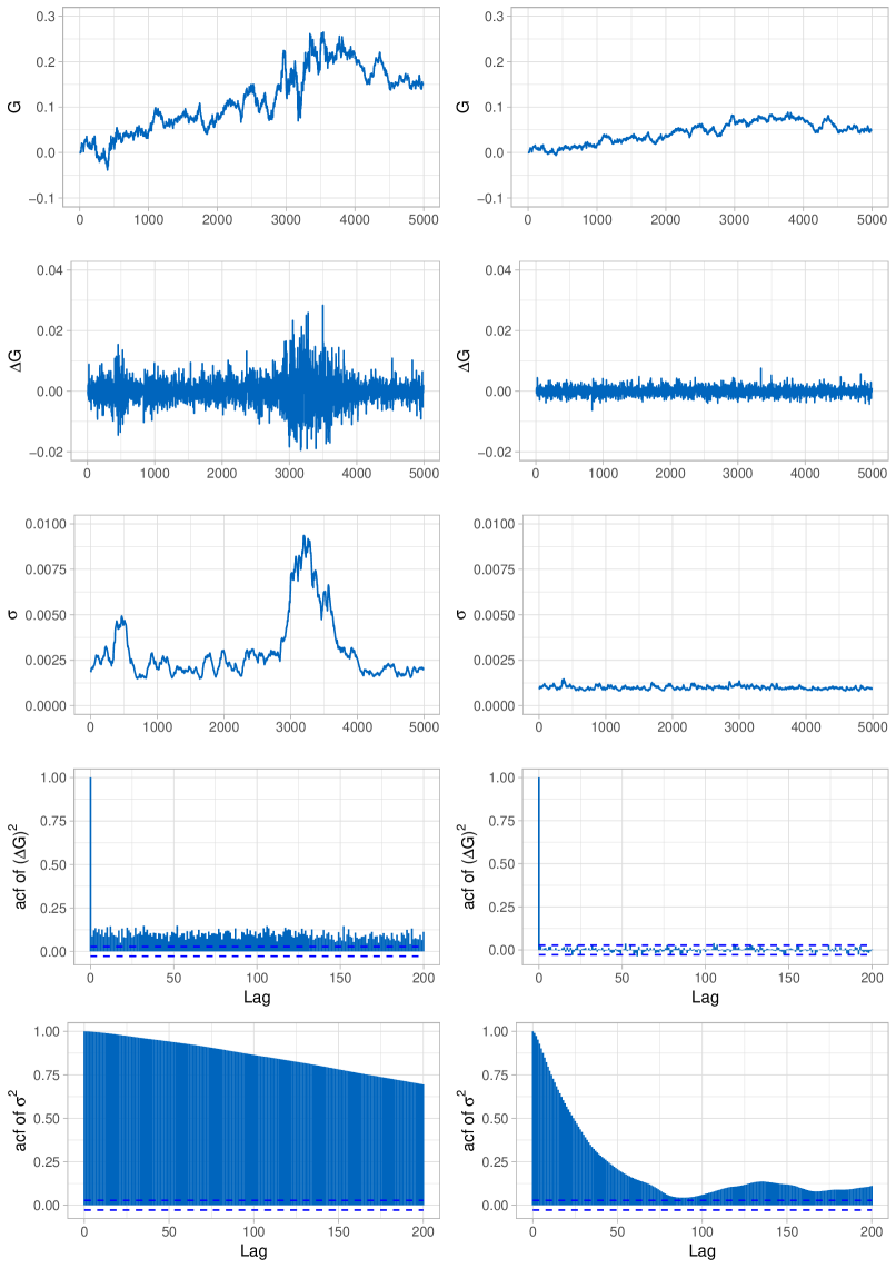
Figure 1: Simulation of the FICOGARCH$(1,d,1)$ process $G$ (top) with corresponding return process $\Delta G$ (second row), volatility process $\sigma$ (third row) and sample acf $\widehat{\gamma}_{\sigma}$ of $\sigma$ (bottom) driven by a compound Poisson process $L$ with rate 5 and normally distributed jump sizes with mean zero and variance one half. The model parameters are $\alpha_{0}=0.0195,\alpha_{1}=0.0105,\beta_{1}=0.0513$ and $a=1.$ The fractional parameter $d$ is equal to $-0.01$ (left) and $-0.4$ (right).

To derive a stationary version of the volatility process in our new model, we need some sample path properties of the fractional subordinator (2.1), which we present in a more general context in the next subsection.

2.1 Sample path properties of fractional subordinators

We first recall from (Cont and Tankov, 2003, Proposition 3.10) that a subordinator $S:=(S_{t})_{t\geq 0}$ is a Lévy process with characteristic triple $(\gamma_{S},0,\nu_{S})$, where $\gamma_{S}\geq 0$ represents the drift of the process, it has no Gaussian component, and its Lévy measure satisfies $\nu_{S}((-\infty,0])=0$, and as a consequence, it has almost surely increasing sample paths of finite variation. In this section we will present some properties of a general fractional subordinator

$$S^{a,d}_{t}=\int_{\mathds{R}}f_{a,d}(t,u)\;\mathrm{d}S_{u},\qquad t\geq 0,$$ (2.7)

where $f_{a,d}$ is the modified MvN kernel and $(S_{t})_{t\in\mathds{R}}$ is a two-sided subordinator defined from $S$ as in (2.2).

The continuity of the sample paths of $(S^{a,d}_{t})_{t\in\mathds{R}}$ will follow from a representation of $S^{a,d}_{t}$ as improper Riemann integral. To derive such a representation, we will use the fact that

$$S_{t}^{a,d}=\begin{cases}\int_{-\infty}^{t}\Big{(}(a+(-s))^{d}-(a+(t-s))^{d}\Big{)}\mathrm{d}S_{s}+\int_{t}^{0}\Big{(}(a+(-s))^{d}-a^{d}\Big{)}\mathrm{d}S_{s}&\mbox{for }t<0,\\ \int_{-\infty}^{0}\Big{(}(a+(-s))^{d}-(a+(t-s))^{d}\Big{)}\mathrm{d}S_{s}+\int_{0}^{t}\Big{(}a^{d}-(a+(t-s))^{d}\Big{)}\mathrm{d}S_{s}&\mbox{for }t\geq 0.\end{cases}$$

The following result is then an analogue of Marquardt (2006b, Theorem 3.4) for a fractional Lévy process.

Proposition 2.3.

Let $S$ be a subordinator with ${\rm{\mathbb{E}}}(S_{1}^{2})<\infty$, $d\in(-0.5,0)$ and $a>0$. Then $(S^{a,d}_{t})_{t\in\mathds{R}}$ as defined in (2.7) has a modification that equals the improper Riemann integral

$$S_{t}^{a,d}=d\int_{\mathds{R}}\Big{(}(a+(-s)_{+})^{d-1}-(a+(t-s)_{+})^{d-1}\Big{)}S_{s}\mathrm{d}s-da^{d-1}\int_{0}^{t}S_{s}\mathrm{d}s,\quad t\in\mathds{R}.$$ (2.8)

Moreover, (2.8) is continuous in $t$ and has sample paths of finite variation.

Recall from Cont and Tankov (2003), Corollary 3.1 and Proposition 3.10, that a subordinator $S$ with strictly increasing sample paths has representation $S_{t}=\gamma_{S}t+\sum_{0<u\leq t}\Delta S_{u}$, for $t\geq 0$; i.e. it has positive drift $\gamma_{S}>0$ and positive jumps of finite variation. If this is the case, then the fractional subordinator $(S_{t}^{a,d})_{t\geq 0}$ also has strictly increasing sample path. This result is summarised in the following proposition. In addition we consider the a.s. limit behaviour of the two-sided process $(S^{a,d}_{t})_{t\in\mathds{R}}$.

Proposition 2.4.

Let $S$ be a subordinator and $d\in(-0.5,0)$ and $a>0$.

1. If $S$ has strictly increasing sample paths, then also $(S^{a,d}_{t})_{t\geq 0}$ has strictly increasing sample paths.

2. The two-sided process $(S^{a,d}_{t})_{t\in\mathds{R}}$ has stationary increments.

3. If ${\rm{\mathbb{E}}}(S_{1})<\infty$, then the following strong law of large numbers (SLLN) holds for the two-sided process $(S_{t}^{a,d})_{t\in\mathds{R}}$:

   $$\lim_{t\to\pm\infty}\frac{1}{|t|}\Big{(}S^{a,d}_{t}-{\rm{\mathbb{E}}}(S_{1})\int_{\mathds{R}}f_{a,d}(t,u)\mathrm{d}u\Big{)}=0\quad\mbox{a.s.}$$ (2.9)

2.2 Stationarity of the FICOGARCH$(1,d,1)$

To construct a stationary version of the FICOGARCH$(1,d,1)$ volatility model, we extend the squared volatility process of (2.4) to the whole of $\mathds{R}$ and use the SLLN from (2.9). In this model the fractional subordinator (2.7) is driven by $S=[L,L]^{(d)}$. Then the auxilliary process (2.6) is extended to

$$X_{t}=\beta_{1}t-\alpha_{1}S_{t}^{a,d}\,,\quad t\in\mathds{R}\,.$$ (2.10)

By Proposition 2.3 $(S^{a,d}_{t})_{t\in\mathds{R}}$ has a modification with finite variational and continuous sample paths, and hence $(X_{t})_{t\in\mathds{R}}$ has.

Proposition 2.5.

Let $S=[L,L]^{(d)}$ be the discrete part of the quadratic variation of a Lévy process $L$. For $d\in(-0.5,0)$ and $a>0$ let $(S_{t}^{a,d})_{t\in\mathds{R}}$ be the fractional subordinator as in (2.7) and $(X_{t})_{t\in\mathds{R}}$ be the auxiliary process from (2.10) and let $\beta_{1}/\alpha_{1}>a^{d}{\rm{\mathbb{E}}}([L,L]_{1}^{(d)})$. Then for $-\infty\leq v<\infty$, the integral

$$\int_{v}^{t}e^{-(X_{t}-X_{s})}\mathrm{d}s,\quad t>v,$$

exists a.s. as a Riemann integral.

Lemma 2.6.

Define

$$\widetilde{\sigma}^{2}_{t}:=\int_{-\infty}^{t}e^{-(X_{t}-X_{s})}\mathrm{d}s\,,\quad t\in\mathds{R}\,.$$

Then for all $t_{1}<\cdots<t_{m}$, $m\in\mathds{N}$, and $h\in\mathds{R}$, we have

$$(\widetilde{\sigma}^{2}_{t_{1}},\ldots,\widetilde{\sigma}^{2}_{t_{m}})\stackrel{{\scriptstyle d}}{{=}}(\widetilde{\sigma}^{2}_{t_{1}+h},\ldots,\widetilde{\sigma}^{2}_{t_{m}+h}).$$

As a consequence of this general result, if in the solution (2.5), we define $\sigma_{0}^{2}:=\alpha_{0}\beta_{1}\int_{-\infty}^{0}e^{X_{s}}\mathrm{d}s$ , we get

$$\sigma_{t}^{2}=\alpha_{0}\beta_{1}\int_{-\infty}^{t}e^{-(X_{t}-X_{s})}\mathrm{d}s\,,\quad t\in\mathds{R},$$

which is a stationary process. The main theorem follows now from the preceding results and the fact that $L$ has independent and stationary increments, which implies stationary increments of the price process $G$ as long as the volatility is a stationary process.

Theorem 2.7.

Let $L$ be a Lévy process with ${\rm{\mathbb{E}}}(L_{1}^{4})<\infty$ and $([L,L]_{t}^{(d)})_{t\in\mathds{R}}$ be the two-sided version of the discrete part of the quadratic variation process of $L$. Let $d\in(-0.5,0)$ and $a>0$ and assume that the parameters $\alpha_{0},\alpha_{1},\beta_{1}>0$ satisfy $\beta_{1}/\alpha_{1}>a^{d}{\rm{\mathbb{E}}}([L,L]_{1}^{(d)})$. Let the squared FICOGARCH$(1,d,1)$ volatility process $(\sigma^{2}_{t})_{t\geq 0}$ be given as in (2.5) with $\sigma_{0}^{2}\stackrel{{\scriptstyle d}}{{=}}\alpha_{0}\beta_{1}\int_{-\infty}^{0}e^{X_{s}}\mathrm{d}s$ independent of $L$. Then $(\sigma^{2}_{t})_{t\geq 0}$ is strictly stationary. Moreover, the process $(G_{t})_{t\geq 0}$ as defined in (2.3) has stationary increments.

Our new approach extends immediately also to higher order COGARCH models.

Remark 2.8.

The COGARCH($p,q$) process was introduced in Brockwell, Chadraa, and Lindner (2006). By the same procedure as above we can generalise the FICOGARCH$(1,d,1)$ model in a straightforward way to its higher order analogue as follows.

Let $p$ and $q$ be integers such that $q\geq p\geq 1$. Further let $\alpha_{0},\alpha_{1},\dots,\alpha_{p}\in\mathds{R},\beta_{1},\dots,\beta_{q}\in\mathds{R},\alpha_{p}\not=0,\beta_{q}\not=0$ and $\alpha_{p+1}=\cdots=\alpha_{q}=0$. Then we define the $q\times q$ matrix $\mathcal{B}$ and the vectors $\mathbf{a}$ and $\mathbf{1}_{q}$ by

$${\mathcal{B}}=\begin{pmatrix}0&1&0&\cdots&0\\ 0&0&1&\cdots&0\\ \vdots&\vdots&\vdots&\ddots&\vdots\\ 0&0&0&\cdots&1\\ -\beta_{q}&-\beta_{q-1}&-\beta_{q-2}&\cdots&-\beta_{1}\end{pmatrix},\ {\mathbf{a}}=\begin{pmatrix}\alpha_{1}\\ \alpha_{2}\\ \vdots\\ \alpha_{q-1}\\ \alpha_{q}\end{pmatrix},\ {\mathbf{1}_{q}}=\begin{pmatrix}0\\ 0\\ \vdots\\ 0\\ 1\end{pmatrix},$$

with $\mathcal{B}:=-\beta_{1}$ if $q=1$. Then for a Lévy proceess $L$ with ${\rm{\mathbb{E}}}(L_{1}^{4})<\infty$, we define the squared volatility process $(\sigma^{2}_{t})_{t\geq 0}$ with parameters $\mathcal{B},{\mathbf{a}},\alpha_{0}$ by

$$\sigma^{2}_{t}=\alpha_{0}+{\mathbf{a}}^{\top}{\mathbf{Y}_{t}},\qquad t\geq 0,$$

where the state process $({\mathbf{Y}}_{t})_{t\geq 0}$ is the unique solution of the SDE

$$\mathrm{d}{\mathbf{Y}}_{t}=\mathcal{B}{\mathbf{Y}}_{t}\mathrm{d}t+{\mathbf{1}_{q}}(\alpha_{0}+{\mathbf{a}}^{\top}{\mathbf{Y}}_{t})\mathrm{d}S_{t}^{a,d},\qquad t>0,$$

with initial value ${\mathbf{Y}}_{0}$, independent of $L$. Furthermore, $(S^{a,d}_{t})_{t\geq 0}$ is the fractional subordinator as defined in equation (2.1). If the process $(\sigma^{2}_{t})_{t\geq 0}$ is strictly stationary and almost surely non-negative, we define the FICOGARCH($p,d,q$) process $(G_{t})_{t\geq 0}$ with parameters $\mathcal{B},{\mathbf{a}},\alpha_{0}$ and some initial value $G_{0}$ as the solution of the SDE

$$\mathrm{d}G_{t}=\sigma_{t}\mathrm{d}L_{t},\qquad t>0.$$

The volatility process of the COGARCH$(1,1)$ and also of the FICOGARCH$(1,d,1)$ is non-negative by definition. This is not necessarily the case for the COGARCH$(p,q)$ model for $q\geq p>1$. Therefore, conditions as formulated in Brockwell et al. (2006, Theorem 5.1) have to be considered to assure non-negativity of the volatility process.

3 An application example

3.1 Parameter estimation

Estimation of the FICOGARCH model is not as straightforward as e.g. for the COGARCH(1,1) model. There the dependence structure of the squared returns $(\Delta G_{\Delta i})^{2}:=(G_{\Delta i}-G_{\Delta(i-1)})^{2}$ is explicitly known and has been used to define a method of moment estimator (Haug et al. (2007)), a prediction based estimator (Bibbona and Negri (2015)), an indirect inference estimator (Do Rego Sousa, Haug, and Klüppelberg (2017)) or a pseudo-maximum-likelihood estimator (Maller, Müller, and Szimayer (2008)).

Fortunately we are able to simulate the FICOGARCH model. This allows us to apply a simulation based version of the generalised method of moments (GMM), due to McFadden (1989). The idea is to compute moments for the observed return data, and match them with empirical moments computed from simulated data of the FICOGARCH model. The method is described in detail in the algorithm below.

We illustrate the estimation for equally spaced observations of the price process $G_{\Delta i},i=0,\ldots,n$, giving return data $\Delta G_{\Delta i}=G_{\Delta i}-G_{\Delta(i-1)},$ $i=1,\ldots,n$, with true parameter $\theta^{0}=(\alpha_{0}^{0},\alpha_{1}^{0},\beta_{1}^{0},d^{0})\in\Theta$, where $\Theta=(0,\infty)^{3}\times(-0.5,0)$ denotes the parameter space.

Algorithm

1. Compute the moment estimator

   $$\widehat{\mu}_{n}:=\frac{1}{n}\sum_{i=1}^{n}(\Delta G_{\Delta i})^{2}$$

   and for fixed $s\geq 3$ the empirical autocovariances $\widehat{\gamma}_{n}:=(\widehat{\gamma}_{n}(0),\widehat{\gamma}_{n}(1),\ldots,\widehat{\gamma}_{n}(s))$ as

   $$\widehat{\gamma}_{n}(h):=\frac{1}{n}\sum_{i=1}^{n-h}\bigg{(}(\Delta G_{\Delta(i+h)})^{2}-\widehat{\mu}_{n}\bigg{)}\bigg{(}(\Delta G_{\Delta i})^{2}-\widehat{\mu}_{n}\bigg{)},\quad h=0,\ldots,s.$$

2. Compute the empirical autocorrelations

   $$\widehat{\rho}_{n}=(\widehat{\rho}_{n}(1),\dots,\widehat{\rho}_{n}(s)):=(\widehat{\gamma}_{n}(1)/\widehat{\gamma}_{n}(0),\ldots,\widehat{\gamma}_{n}(s)/\widehat{\gamma}_{n}(0)).$$

3. For $\theta=(\alpha_{0},\alpha_{1},\beta_{1},d)\in\Theta$ simulate a sample path $(\Delta G_{\Delta i}(\theta))_{i=0,\ldots,n}$ of return data.
   Repeat steps (1) and (2) to obtain $\widehat{\mu}_{n,\theta}$ and $\widehat{\rho}_{n,\theta}$.

4. Define the function $\mathcal{L}^{(s)}(\theta)$ by

   $$\mathcal{L}^{(s)}(\theta)=\sum_{h=1}^{s}(\widehat{\rho}_{n,\theta}(h)-\widehat{\rho}_{n}(h))^{2}+(\widehat{\mu}_{n,\theta}-\widehat{\mu}_{n})^{2}$$ (3.1)

   The simulation-based GMM estimator $\widehat{\theta}_{n}$ of $\theta^{0}$ is given by:

   $$\widehat{\theta}_{n}=\mathrm{argmin}_{\theta\in\Theta}\mathcal{L}^{(s)}(\theta).$$

Before commenting on some practical issues of the above algorithm we present a useful simplification.

Lemma 3.1.

Let $\Delta G_{t}=G_{t}-G_{t-\Delta}$ be an increment of a stationary FICOGARCH$(1,d,1)$ process with parameter $(\alpha_{0},\alpha_{1},\beta_{1},d)$ satisfying the conditions of Theorem 2.7. Then, for any $k>0$, the scaled increment $k\cdot\Delta G_{t}$ has the same distribution as the increment of a FICOGARCH$(1,d,1)$ with parameter $(k^{2}\alpha_{0},\alpha_{1},\beta_{1},d)$.

This result follows from the fact that the stationary squared volatility process of the scaled FICOGARCH$(1,d,1)$ process $(kG_{t})_{t\geq 0}$ is given by

$$(k\sigma_{t})^{2}=k^{2}\alpha_{0}\beta_{1}\int_{-\infty}^{t}e^{-(X_{t}-X_{s})}\mathrm{d}s,\qquad t\in\mathds{R}.$$

Since $(X_{t})_{t\in\mathds{R}}$ is independent of $\alpha_{0}$, it follows that

$$\Delta G(\alpha_{0},\alpha_{1},\beta_{1},d)\overset{d}{=}\sqrt{\alpha_{0}}\Delta G(1,\alpha_{1},\beta_{1},d)\,.$$

Hence, $\rho_{[\Delta G(\alpha_{0},\alpha_{1},\beta_{1},d)]^{2}}(h)=\rho_{[\Delta G(1,\alpha_{1},\beta_{1},d)]^{2}}(h)$ for every $h\geq 0$, where $\rho_{[\Delta G(\theta)]^{2}}$ denotes the autocorrelation function of squared increments of a stationary FICOGARCH$(1,d,1)$ process with parameter $\theta$.

The minimisation of the score function (3.1) is therefore performed in two steps. First we keep $\alpha_{0}=1$ fixed and minimise the first term in (3.1) with respect to $(\alpha_{1},\beta_{1},d)$. Second, since we have $\widehat{\mu}_{n,(\alpha_{0},\alpha_{1},\beta_{1},d)}=\alpha_{0}\widehat{\mu}_{n,(1,\alpha_{1},\beta_{1},d)}$ by Lemma 3.1, the second term in (3.1) is minimised by choosing:

$$\widehat{\alpha}_{0}=\frac{\widehat{\mu}_{n}}{\widehat{\mu}_{n,(1,\widehat{\alpha}_{1},\widehat{\beta}_{1},\widehat{d})}}\,.$$

We now proceed to investigate the small sample behaviour of the proposed estimator. We simulate 5 000 equidistant observations of $\Delta G$ with $\Delta=1$. The driving Lévy process $L$ is compound Poisson with rate one and standard normally distributed jumps. The cut-off for the computation of the empirical acf has been chosen as $s=80$ lags. Table 1 summarises the estimation results for $N=100$ simulation runs. The five examples shown in the table only differ in $d$, which varies between -0.01 and -0.49 as indicated in the right column of the table. The estimation of the parameters $\beta_{1}$ and $d$ becomes less efficient as $d$ decreases towards $-0.49$. This is due to the fact that, when $d$ decreases, the model becomes less dependent so that the acf of the squared returns is less informative about the model parameters. The estimation results for the other two parameters are not affected by the decrease of $d$ and are overall satisfying.

	$\alpha_{0}$	$\alpha_{1}$	$\beta_{1}$	$d$
TrueValue	0.04000	0.08000	0.34000	-0.01000
Mean	0.05093 (0.01932)	0.09080 (0.03621)	0.35720 (0.16520)	-0.14400 (0.14914)
RMSE	0.00049	0.00143	0.02759	0.04020
TrueValue	0.04000	0.08000	0.34000	-0.10000
Mean	0.04218 (0.02751)	0.08920 (0.03045)	0.31720 (0.12431)	-0.12400 (0.13566)
RMSE	0.00076	0.00101	0.01597	0.01898
TrueValue	0.04000	0.08000	0.34000	-0.25000
Mean	0.04798 (0.01267)	0.13640 (0.07894)	0.57480 (0.31452)	-0.29400 (0.16169)
RMSE	0.00022	0.00941	0.15405	0.02808
TrueValue	0.04000	0.08000	0.34000	-0.40000
Mean	0.05028 (0.01425)	0.10920 (0.09130)	0.72360 (0.29278)	-0.29400 (0.16415)
RMSE	0.00031	0.00919	0.23287	0.03818
TrueValue	0.04000	0.08000	0.34000	-0.49000
Mean	0.04802 (0.01293)	0.09800 (0.09364)	0.73640 (0.30812)	-0.27400 (0.17523)
RMSE	0.00023	0.00909	0.25207	0.07736

Table 1: Empirical mean, standard deviation (in brackets) and root mean squared error (RMSE) of the estimated FICOGARCH$(1,d,1)$ parameters.

3.2 The FICOGARCH model fitted to FOREX data

The FICOGARCH$(1,d,1)$ model has been fitted to log-returns of two different exchange rate data, namely EUR (Euro)/USD (United States Dollar) and GBP (British Pound)/USD. The data set have a total length of 4 436 (from December 10, 1999 to December 12, 2016) and 10 436 (from December 10, 1976 to December 12, 2016) data points, respectively.

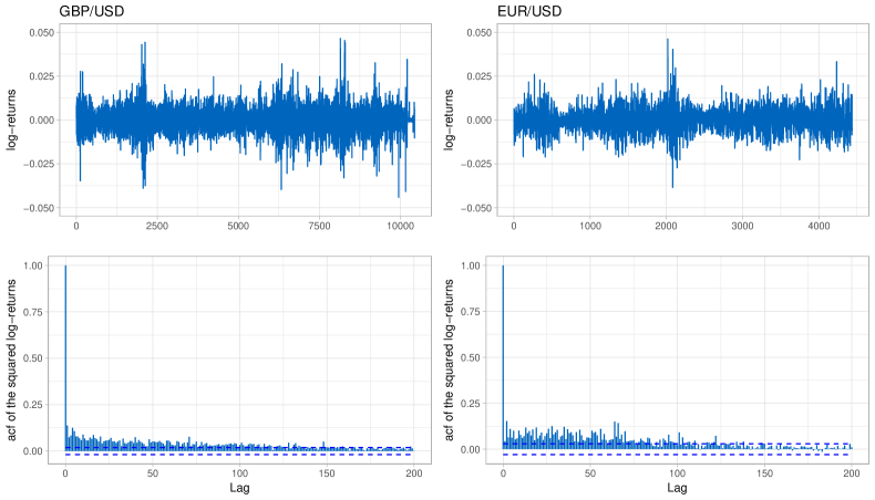
Figure 2: Log-returns of foreign exchange rates (top) and sample acf of squared log-returns (bottom) for GBP/USD (left) and USD/EUR (right) exchange rates.

The sample autocorrelation function of the squared log-returns indicates some moderately long memory behaviour as it is described by the FICOGARCH model; cf. the corresponding plots in Figure 1.

We applied the Algorithm of Section 3.1 to each data set to estimate the parameters $\alpha_{0},\alpha_{1},\beta_{1}$ and $d$ of the FICOGARCH(1,d,1) model. The parameter $a$ of the fractional process $(S^{a,d}_{t})_{t\in\mathds{R}}$ was set equal to 1 in both cases. For the simulation part the driving Lévy process $L$ was chosen to be a compound Poisson process with rate one and standard normally distributed jumps. The estimated parameters are shown in Table 2. The last column represents the realised minimum of the score function $\mathcal{L}^{(s)}(\hat{\theta})$.

	$\widehat{\alpha}_{0}$	$\widehat{\alpha}_{1}$	$\widehat{\beta}_{1}$	$\widehat{d}$	$\mathcal{L}^{(s)}(\hat{\theta})$
GBP/USD	1.7656e-6	0.0274	0.1099	-0.0300	0.0830
EUR/USD	1.2295e-5	0.0390	0.1460	-0.0150	0.1607

Table 2: Parameter estimates $\widehat{\alpha}_{0}$, $\widehat{\alpha}_{1}$, $\widehat{\beta}_{1}$, $\widehat{d}$ for GBP/USD and EUR/USD exchange rate data.

The estimated values of $d$ are rather close to 0 for both series, which indicates that the fitted FICOGARCH model has an acf with a rather slow decay. The estimated models are stationary, since the ratios $0.1099/0.0274$ and $0.1460/0.0390$ are both larger than $1=a^{\widehat{d}}{\rm{\mathbb{E}}}([L,L]_{1})$. The estimates for $\alpha_{0}$ are both close to zero, which is due to the scale of the data (cf. Lemma 3.1).

4 Fractional subordinators in stochastic volatility models

In this section we discuss the fractional subordinator as defined in (2.7) with its specification (2.1) as driving process of the FICOGARCH$(1,d,1)$ squared volatility. The non-negativity needed for the squared volatility can be achieved in various ways, one possibility consists in the integral transform of a subordinator with a positive kernel as the Ornstein-Uhlenbeck type volatility model of Barndorff-Nielsen and Shephard (2001). Long range dependence is then introduced by replacing the OU kernel by a fractional kernel as suggested for instance in Anh et al. (2002), or by taking the integral transform of a fractional subordinator with an appropriate kernel as in Brockwell and Marquardt (2005), Section 8. Also time-changed subordinators as in Carr, Geman, Madan, and Yor (2003) can be modified to introduce long range dependence. Bender and Marquardt (2009) replaces classical time-change models by the integral transform of a subordinator with a MG-kernel as in (1.5) which, when used as a random time change process, also results in a long range dependence model.

As explained in Section 1.2, the classical MG-kernel in (1.5) and MvN-kernel in (1.6) have certain drawbacks, which make them inappropriate for fractional subordinator modelling for long range dependence in stochastic volatility. The MG-fractional subordinator $(\tilde{L}_{t}^{d})_{t\geq 0}$ defined in (1.8) does not necessarily lead to stationarity of the squared volatility process. The MvN-fractional subordinator $(L^{d}_{t})_{t\in\mathds{R}}$ defined in (1.8) is well-defined for any subordinator $S$, if $d\in(-0.5,0)$. But due to the singularity at $s=t$ $(S^{d}_{t})_{t\in\mathds{R}}$ has discontinuous and unbounded sample paths with positive probability (cf. Rosinski (1989, Theorem 4)). To overcome these drawbacks, we bound the MvN-kernel at its singularities.

Observe that for every $t\in\mathds{R}$ the MvN-kernel $f^{MvN}_{d}(t,\cdot)$ is up to a constant given by the function $s\mapsto g_{d}(t-s)-g_{d}(-s)$, where $g_{d}$ is defined by $g_{d}(x):=x^{d}_{+}$. This suggests to bound $g_{d}$ at its singularities $s=0$ and $s=t$ by incorporating a shift $a>0$, leading to the following definition of a modification of the Mandelbrot-van-Ness kernel.

Definition 4.1.

Let $d\in(-0.5,0)$ and $a>0$. For each $t\in\mathds{R}$ the (non-normalised) modified MvN-kernel is given by

$$\begin{aligned} f_{a,d}(t,s)&=g_{a,d}(-s)-g_{a,d}(t-s)\\ &:=\left(a+(-s)_{+}\right)^{d}-\left(a+(t-s)_{+}\right)^{d},\qquad s\in\mathds{R}.\end{aligned}$$ (4.1)

Figure 3: Left: Comparison of the MvN kernel $f^{MvN}_{d}(t,\cdot)$ and the modified MvN kernel $f_{a,-d}(t,\cdot)$ for $d=0.25,a=0.1$. Right: Modified MvN kernel $f_{a,d}(t,\cdot)$ with $d=-0.25$ for different values of the shift parameter $a$ for $t=15$.

Some properties of the new kernel are summarised in the next proposition.

Proposition 4.2.

For $d\in(-0.5,0)$ and $a>0$ consider the modified MvN-kernel $f_{a,d}$ as in (4.1). Then the following holds.

1. $f_{a,d}(t,\cdot)\geq 0$ for all $t\geq 0$,

2. $f_{a,d}(t,\cdot)$ is continuous for all $t\in\mathds{R}$,

3. $|f_{a,d}(t,s)|\leq a^{d}$ for all $t,s\in\mathds{R}$,

4. $|f_{a,d}(t,s)|\sim|s|^{d-1}|dt|$  as $s\to-\infty$ (equivalently, $\lim\limits_{s\to-\infty}{|f_{a,d}(t,s)|}/{(|s|^{d-1}|dt|)}=1$) for all $t\in\mathds{R}$.

5. $f_{a,d}(t,\cdot)\in L^{\delta}(\mathds{R})$ for all $\delta>1/|d-1|$; in particular, $f_{a,d}(t,\cdot)\in L^{1}(\mathds{R})\cap L^{2}(\mathds{R})$ for all $t\in\mathds{R}$.

The new kernel can now be used to define a fractional subordinator analogously to (1.8). The existence of such an integral is shown in the following proposition.

Proposition 4.3.

Let $a>0$ and $d\in(-0.5,0)$, and let $S$ be a subordinator satisfying ${\rm{\mathbb{E}}}(S_{1}^{2})<\infty$. Then the fractional subordinator

$$S^{a,d}_{t}=\int_{\mathds{R}}f_{a,d}(t,u)\;\mathrm{d}S_{u}$$ (4.2)

exists for all $t\in\mathds{R}$ as limit in the $L^{2}(\Omega)$-sense and hence in probability.

Remark 4.4.

Some related kernels have been used in the literature, and we want to comment on some of them.

• For comparison, recall from above that the MvN kernel is for $d\in(-0.5,0)$ and $t\in\mathds{R}$ defined as

  $$f^{MvN}_{d}(t,s)=\frac{1}{\Gamma(1+d)}(g_{d}(t-s)-g_{d}(-s))=\frac{-1}{\Gamma(1+d)}\frac{\mathrm{d}}{\mathrm{d}s}\int_{s}^{\infty}\mathds{1}_{(0,t)}(v)(v-s)^{d}\mathrm{d}v,\quad t,s\in\mathds{R},$$

  see Mishura (2008, Lemma 1.1.3). As it is in $L^{2}(\mathds{R})$, this kernel can generate fBm and fLm on $\mathds{R}$ for symmetric driving processes.

• The approach in Brockwell and Marquardt (2005) to construct a FICARMA process driven by a subordinator suggests to use the kernel

  $$\frac{-1}{\Gamma(1+d)}\frac{\mathrm{d}}{\mathrm{d}s}\int_{s}^{\infty}\mathds{1}_{(0,t)}(v)\min(a^{d},(v-s)^{d})\mathrm{d}v,\quad t,s\in\mathds{R},$$

  for $d\in(-0.5,0)$ and some $a>0$. For us it was computationally advantageous to bound $g_{d}$ and not the integrand in the above representation.

• Meerschaert and Sabzikar (2014) suggest a tempered fractional kernel of the form

  $$f_{d}^{\rm temp}(t,s):=e^{-\lambda(t-s)_{+}}(t-s)_{+}^{d}-e^{-\lambda(-s)_{+}}(-s)_{+}^{d},\quad t,s\in\mathds{R},$$

  for $d>-0.5$ and $\lambda>0$, which also has an integral representation using tempered fractional integrals, see Meerschaert and Sabzikar (2014, Definition 2.1) for details. For every $t\in\mathds{R}$ the kernel $f_{d}^{\rm temp}(t,\cdot)$ belongs to $L^{p}(\mathds{R})$ for all $p\geq 1$. The autocovariance function of the increments of the corresponding tempered fractional process decreases for small lags algebraically, but for large lags exponentially. It is therefore called a semi-long range dependence model.

• Klüppelberg and Matsui (2015) generalise fLp’s by allowing the kernel to be regularly varying, which results in functional central limit theorems for scaled Ornstein-Uhlenbeck processes driven by such generalized fLp’s.

4.1 Cumulant generating function and moments

Let $S$ be a subordinator without drift, then its cumulant generating function is given by $\ln{\rm{\mathbb{E}}}(e^{hS_{1}})=\int_{0}^{\infty}(e^{hz}-1)\nu_{S}(\mathrm{d}z)$, where $\nu_{S}$ is the Lévy measure of $S$ (see Chapter 4.2.2 in Cont and Tankov (2003)). Rajput and Rosinski (1989, Proposition 2.6) expresses the cumulant generating function of $(S^{a,d}_{t})_{t\in\mathds{R}}$ as

$$\ln{\rm{\mathbb{E}}}(e^{hS_{t}^{a,d}})=\ln{\rm{\mathbb{E}}}\Big{(}\exp\Big{\{}h\int_{\mathds{R}}f_{a,d}(t,u)\;\mathrm{d}S_{u}\Big{\}}\Big{)}=\int_{\mathds{R}}\int_{0}^{\infty}(e^{hf_{a,d}(t,u)z}-1)\nu_{S}(\mathrm{d}z)\mathrm{d}u.$$

The $k$-th cumulant of $S_{t}^{a,d}$ is then given by $\kappa^{k}(S_{t}^{a,d})=\frac{d^{k}}{dh^{k}}\ln{\rm{\mathbb{E}}}(e^{hS_{t}^{a,d}})\big{|}_{h=0}$. For the $k$-th derivative in 0 we obtain, provided the corresponding Lévy cumulant exists,

$$\kappa^{k}(S_{t}^{a,d})=\int_{0}^{\infty}z^{k}\nu_{S}(\mathrm{d}z)\int_{\mathds{R}}f_{a,d}^{k}(t,u)\mathrm{d}u=\kappa^{k}(S_{1})\int_{\mathds{R}}f_{a,d}^{k}(t,u)\mathrm{d}u.$$

where the integral exists by Proposition 4.2 (v) for all $k>1$. From this we calculate the mean and variance as

$${\rm{\mathbb{E}}}(S_{t}^{a,d}) ={\rm{\mathbb{E}}}(S_{1})\int_{\mathds{R}}f_{a,d}(t,u)\mathrm{d}u,$$

$${\rm{\mathbb{V}}ar}(S_{t}^{a,d}) ={\rm{\mathbb{V}}ar}(S_{1})\int_{\mathds{R}}f_{a,d}^{2}(t,u)\mathrm{d}u.$$

4.2 Properties of the increments of the fractional subordinator

Next we ask whether $f_{a,d}$ serves its purpose in the sense that the increments of $(S^{a,d}_{t})_{t\in\mathds{R}}$ exhibit a long range dependence structure. We start with an auxiliary result.

Lemma 4.5.

Let $d\in(-0.5,0)$ and $a>0$. Then the modified MvN-kernel $f_{a,d}(t,\cdot)$ as in (4.1) satisfies for $t>0$

$$\int_{\mathds{R}}f_{a,d}^{2}(t,u)\;\mathrm{d}u=C+a^{2d}\;t-\frac{2a^{d}}{d+1}(t+a)^{d+1}+\frac{1}{2d+1}(t+a)^{2d+1}+c(t)t^{2d+1}$$

with

$$C=a^{2d+1}\Big{(}\dfrac{2}{d+1}-\dfrac{1}{2d+1}\Big{)}\quad\mbox{and}\quad c(t)=\int_{-\infty}^{-a/t}\left[(1-y)^{d}-(-y)^{d}\right]^{2}\;dy,$$ (4.3)

and

$$\lim_{t\to\infty}c(t)=\frac{\Gamma(d+1)}{\Gamma(2d+2)\sin(\pi(d+0.5))}+\frac{1}{2d+1}.$$ (4.4)

From this we are able to derive the asymptotic behaviour of the autocovariance function of the increments of $(S^{a,d}_{t})_{t\in\mathds{R}}$.

Proposition 4.6.

Let $d\in(-0.5,0)$ and $a>0$, and let $S$ be a subordinator satisfying ${\rm{\mathbb{E}}}(S_{1}^{2})<\infty$. Let $(S^{a,d}_{t})_{t\in\mathds{R}}$ be as defined in (4.2), then the following holds. Let $\Delta>0$ be fixed and $s+\Delta\leq t$ such that $t-s=h\Delta$ for some $h>0$. Then the two increments $S^{a,d}_{t+\Delta}-S^{a,d}_{t}$ and $S^{a,d}_{s+\Delta}-S^{a,d}_{s}$ of length $\Delta$ have covariance

$$\gamma_{\Delta}(h):={\rm{\mathbb{C}}ov}\left(S^{a,d}_{s+(h+1)\Delta}-S^{a,d}_{s+h\Delta},S^{a,d}_{s+\Delta}-S^{a,d}_{s}\right),$$

which satisfies

$$\gamma_{\Delta}(h)\sim{\rm{\mathbb{V}}ar}\big{(}S_{1}\big{)}|d|a^{d}\Delta^{2}\;(h\Delta+a)^{d-1},\quad h\to\infty.$$

The increments of $(S^{a,d}_{t})_{t\in\mathds{R}}$ do not have long memory in the standard sense, since the autocovariance function is integrable. However, it decreases algebraically, and for $d$ close to zero we approximately obtain long memory. This is in analogy to the asymptotic rate of decay of the modified CARMA kernel $g_{a,d}$ in the case of subordinator-driven CARMA processes as in Brockwell and Marquardt (2005, Section 8).

5 Conclusion and outlook

We have introduced a new FICOGARCH$(1,d,1)$ model, which is strictly stationary and exhibits an algebraic decay in its autocovariances. Moreover, we have shown how to extend this model to a FICOGARCH$(p,d,q)$ process of arbitrary order. The properties of the model present it as an appropriate model for high-frequency financial data exhibiting moderate long memory. We have also presented a simple estimation method for the model parameters including the fractional parameter, which works well in a simulation study. We have also applied this method to exchange rate data. More sophisticated estimation procedures are envisaged like the estimation of $d$ in a preliminary step by an appropriate estimator. Then in a second step the FICOGARCH parameters can be estimated by modified COGARCH estimators as suggested in Bibbona and Negri (2015), Haug et al. (2007), Maller et al. (2008), or Do Rego Sousa et al. (2017). This is a version of the semiparametric approach suggested in Robinson (1994). Alternatively, a quasi-maximum likelihood estimation as in Tsai and Chan (2005) can be applied to estimate $d$ and all model parameters in one go.

Appendix A Appendix

Proofs of Section 2

Proof of Proposition 2.3.

First note that for every finite variational sample path of $(S^{a,d}_{t})_{t\in\mathds{R}}$ we can apply partial integration and obtain for $t>0$

$$S_{t}^{a,d} =\lim_{u\to-\infty}\int_{u}^{0}\Big{(}(a+(-s))^{d}-(a+(t-s))^{d}\Big{)}\mathrm{d}S_{s}+\int_{0}^{t}\Big{(}a^{d}-(a+(t-s))^{d}\Big{)}\mathrm{d}S_{s}$$

$$=-(a^{d}-(a+t)^{d})S_{0}-d\int_{0}^{t}(a+(t-s))^{d-1}S_{s}\mathrm{d}s+(a^{d}-(a+t)^{d})S_{0}$$

$$\quad-\lim_{u\to-\infty}\Big{(}(a+(-u))^{d}-(a+(t-u))^{d}\Big{)}S_{u}$$

$$\quad+\lim_{u\to-\infty}d\int_{u}^{0}\Big{(}(a+(-s))^{d-1}-(a+(t-s))^{d-1}\Big{)}S_{s}\mathrm{d}s$$ (A.1)

Now recall that by the SLLN (cf. Sato (1999, Proposition 36.3)) that

$$\lim_{s\to-\infty}\frac{S_{s}}{|s|}\rightarrow{\rm{\mathbb{E}}}(S_{1})\quad a.s.$$

Therefore, we get

$$0 \leq\lim_{u\to-\infty}\Big{(}(a+(-u))^{d}-(a+(t-u))^{d}\Big{)}S_{u}\leq\lim_{u\to-\infty}dt\,(a-u)^{d-1}\,S_{u}$$

$$=\lim_{u\to-\infty}dt\frac{S_{u}}{|u|}\,\Big{(}1-\frac{a}{u}\Big{)}^{-1}\,(a-u)^{d}=0\,,$$

and, thus, the limit integral in (A) is finite. This yields

$$S_{t}^{a,d}=d\int_{-\infty}^{0}\Big{(}(a-s)^{d-1}-(a+(t-s))^{d-1}\Big{)}S_{s}\mathrm{d}s-d\int_{0}^{t}(a+(t-s))^{d-1}S_{s}\mathrm{d}s.$$

For $t\leq 0$ we get analogously

$$S_{t}^{a,d}=d\int_{-\infty}^{t}\Big{(}(a-s)^{d-1}-(a+(t-s))^{d-1}\Big{)}S_{s}\mathrm{d}s+d\int_{t}^{0}(a-s)^{d-1}S_{s}\mathrm{d}s.$$

Continuity follows from dominated convergence from Proposition 4.2 (iii). Since the kernel $f_{a,d}(t,\cdot)$ and almost all paths of $(S_{t})_{t\in\mathds{R}}$ have finite variation, it follows that also $(S^{a,d}_{t})_{t\in\mathds{R}}$ has sample paths of finite variation. ∎

Proof of Proposition 2.4.

(i)  For $t\geq 0$ we have the representation

$$S_{t}^{a,d}=\int_{-\infty}^{0}\Big{(}(a+(-s))^{d}-(a+(t-s))^{d}\Big{)}\mathrm{d}S_{s}+\int_{0}^{t}\Big{(}a^{d}-(a+(t-s))^{d}\Big{)}\mathrm{d}S_{s}\,.$$

The functions $t\mapsto\big{(}(a+(-s))^{d}-(a+(t-s))^{d}\big{)}\mathds{1}_{(-\infty,0)}(s)$ and $t\mapsto\big{(}a^{d}-(a+(t-s))^{d}\big{)}\mathds{1}_{(0,t)}(s)$ are for each fixed $s$ positive. Therefore, it follows from the above representation that $(S^{a,d}_{t})_{t\in\mathds{R}}$ has strictly increasing sample path if $(S_{t})_{t\in\mathds{R}}$ has strictly increasing sample path.

(ii) For $n\in\mathds{N}$, $t_{0}<t_{1}<\cdots<t_{n}$ and $a_{1},\ldots,a_{n}\in\mathds{R}$ we use the Cramér-Wold device and calculate

$$\sum_{i=1}^{n}a_{i}(S^{a,d}_{t_{i}+h}-S^{a,d}_{t_{i-1}+h}) = \sum_{i=1}^{n}a_{i}\int_{\mathds{R}}(g_{a,d}(t_{i-1}+h-u)-g_{a,d}(t_{i}+h-u))\mathrm{d}S_{u}$$

$$\stackrel{{\scriptstyle d}}{{=}} \sum_{i=1}^{n}a_{i}\int_{\mathds{R}}(g_{a,d}(t_{i-1}-v)-g_{a,d}(t_{i}-v))\mathrm{d}S_{v}$$

$$= \sum_{i=1}^{n}a_{i}(S^{a,d}_{t_{i}}-S^{a,d}_{t_{i-1}}),$$

where we have used the stationary increments of $(S_{t})_{t\in\mathds{R}}$.

(iii) We will only consider the case $t\rightarrow-\infty$. The result for $t\rightarrow\infty$ follows by analogous arguments. In the first step, we prove that a SLLN holds for $\tilde{S}^{a,d}_{t}:=\int_{\mathds{R}}f_{a,d}(t,u)\;d\tilde{S}_{u}$ with

$$\tilde{S}_{t}:=S_{t}-{\rm{\mathbb{E}}}\big{(}S_{t}\big{)}=S_{t}-{\rm{\mathbb{E}}}\big{(}S_{1}\big{)}t\,;$$ (A.2)

i.e., that $\lim_{t\to-\infty}\tilde{S}^{a,d}_{t}/t=0$ a.s.. The proof is a modification of the proof of Fink and Klüppelberg (2011, Theorem 3.1).

Without loss of generality we assume that $t<0$. By the law of the iterated logarithm (LIL) for Lévy processes (cf. Sato (1999), Proposition 48.9) we find a random variable $T$ and a constant $M>0$ such that a.s. for all $s<T$

$$|\tilde{S}_{s}|\leq M(2|s|\log\log|s|)^{\frac{1}{2}}.$$

We can always make $T$ smaller and so we choose $T<-e$. For any such path we can assume that $t<T$ and, since (2.8) holds for $\tilde{S}^{a,d}$, we calculate

$$\tilde{S}^{a,d}_{t} =d\int_{-\infty}^{\infty}\Big{(}(a+(-s)_{+})^{d-1}-(a+(t-s)_{+})^{d-1}\Big{)}\tilde{S}_{s}\mathrm{d}s+da^{d-1}\int_{t}^{0}\tilde{S}_{s}\mathrm{d}s$$

$$=d\int_{-\infty}^{t}\Big{(}(a+(-s))^{d-1}-(a+(t-s))^{d-1}\Big{)}\tilde{S}_{s}\mathrm{d}s+d\int_{t}^{0}\Big{(}(a+(-s))^{d-1}-a^{d-1}\Big{)}\tilde{S}_{s}\mathrm{d}s$$

$$\quad+da^{d-1}\int_{t}^{0}\tilde{S}_{s}\mathrm{d}s\,.$$

It suffices to show that

$$\lim_{t\rightarrow-\infty}\frac{1}{|t|}\int_{-\infty}^{t}\Big{(}(a+(-s))^{d-1}-(a+(t-s))^{d-1}\Big{)}|\tilde{S}_{s}|\mathrm{d}s=0\quad a.s.,$$ (A.3)

and

$$\lim_{t\rightarrow-\infty}\frac{1}{|t|}\int_{t}^{0}(a+(-s))^{d-1}|\tilde{S}_{s}|\mathrm{d}s=0\quad a.s.$$ (A.4)

We start with (A.3). Using the LIL we get an upper bound as follows

$$\frac{1}{|t|}\int_{-\infty}^{t}\Big{(}(a+(-s))^{d-1}-(a+(t-s))^{d-1}\Big{)}|\tilde{S}_{s}|\mathrm{d}s$$

$$\leq\frac{M}{|t|}\int_{-\infty}^{-|t|}\Big{(}(a+(-s))^{d-1}-(a+(t-s))^{d-1}\Big{)}(2|s|\log\log|s|)^{\frac{1}{2}}\mathrm{d}s$$

$$=\frac{M}{|t|}\int_{-\infty}^{-|t|-a}\Big{(}(-v)^{d-1}-(-v-|t|)^{d-1}\Big{)}(2|v+a|\log\log|v+a|)^{\frac{1}{2}}\mathrm{d}v$$

$$=\frac{M|t|}{e|t|}\int_{-\infty}^{-e}\Big{(}(-e^{-1}|t|u-a)^{d-1}-(-|t|-e^{-1}|t|u-a)^{d-1}\Big{)}(2(e^{-1}|t||u|)\log\log\big{(}\frac{|t||u|}{e}\big{)})^{\frac{1}{2}}\mathrm{d}u,$$ (A.5)

where we have used in the last line the change of variable $e^{-1}|t|u-a=v$.

Now note that for large $|t|$ and $|u|\geq e$

$$|t||u|\log\log(e^{-1}|t||u|) =|t||u|\log(\log(e^{-1}|t|)+\log|u|)$$ (A.6)

$$\leq|t||u|\log\log|t|+|t||u|\log(1+\log|u|)\,.$$

Combining $(\ref{FLP24b})$ with $|a+b|^{\frac{1}{2}}\leq|a|^{\frac{1}{2}}+|b|^{\frac{1}{2}}$ for $a,b\in\mathbb{R}$ we get an upper bound for $(\ref{FLP24c})$ by

$$\frac{M(2e^{-1}|t|\log\log|t|)^{\frac{1}{2}}}{e|t|^{1-d}}\int_{-\infty}^{-e}\Big{(}(-e^{-1}u-\frac{a}{|t|})^{d-1}-(-1-e^{-1}u-\frac{a}{|t|})^{d-1}\Big{)}|u|^{\frac{1}{2}}\mathrm{d}u$$

$$\qquad+\frac{M(2e^{-1}|t|)^{\frac{1}{2}}}{e|t|^{1-d}}\int_{-\infty}^{-e}\Big{(}(-e^{-1}u-\frac{a}{|t|})^{d-1}-(-1-e^{-1}u-\frac{a}{|t|})^{d-1}\Big{)}(|u|\log(1+\log|u|))^{\frac{1}{2}}\mathrm{d}u$$

$$=\frac{M(2e^{-1}\log\log|t|)^{\frac{1}{2}}}{e|t|^{1-(d+\frac{1}{2})}}\int_{e}^{\infty}\Big{(}(e^{-1}u-\frac{a}{|t|})^{d-1}-(e^{-1}u-1-\frac{a}{|t|})^{d-1}\Big{)}u^{\frac{1}{2}}\mathrm{d}u$$

$$\qquad+\frac{M(2e^{-1})^{\frac{1}{2}}}{e|t|^{1-(d+\frac{1}{2})}}\int_{e}^{\infty}\Big{(}(e^{-1}u-\frac{a}{|t|})^{d-1}-(e^{-1}u-1-\frac{a}{|t|})^{d-1}\Big{)}(u\log(1+\log u))^{\frac{1}{2}}\mathrm{d}u\,.$$ (A.7)

By a binomial expansion we get

$$(e^{-1}u-\frac{a}{|t|}-1)^{d-1}=(e^{-1}u-\frac{a}{|t|})^{d-1}-(d-1)(e^{-1}u-\frac{a}{|t|})^{d-2}+\mathcal{O}(u^{d-3})$$

and, therefore, (writing $a(u)\sim b(u)$ for $\lim_{u\to\infty}a(u)/b(u)=1$)

$$\left[(e^{-1}u-\frac{a}{|t|})^{d-1}-(e^{-1}u-\frac{a}{|t|}a-1)^{d-1}\right](u\log(1+\log|u|))^{\frac{1}{2}}$$

$$\sim(d-1)(e^{-1})^{d-2}u^{d-\frac{3}{2}}(\log\log(u))^{\frac{1}{2}}\,,$$

which ensures the existence of the two integrals in $(\ref{FLP24w})$. Letting $t\to-\infty$ we obtain (A.3).
Next we calculate

$$\frac{1}{|t|}\int_{t}^{0}(a+(-s))^{d-1}|\tilde{S}_{s}|\mathrm{d}s=\frac{1}{|t|}\int_{t}^{T}(a+(-s))^{d-1}|\tilde{S}_{s}|\mathrm{d}s+\frac{1}{|t|}\int_{T}^{0}(a+(-s))^{d-1}|\tilde{S}_{s}|\mathrm{d}s$$

The second term tends to zero as $t\to-\infty$, and we consider the first:

$$\frac{1}{|t|}\int_{t}^{T}(a+(-s))^{d-1}|\tilde{S}_{s}|\mathrm{d}s \leq\frac{M}{|t|}\int_{t}^{T}(a+(-s))^{d-1}(2|s|\log\log|s|)^{\frac{1}{2}}\mathrm{d}s$$

$$\leq\frac{M(2|t|\log\log|t|)^{\frac{1}{2}}}{|t|}\int_{t}^{T}(a+(-s))^{d-1}\mathrm{d}s$$

$$\leq\frac{M(2\log\log|t|)^{\frac{1}{2}}}{|t|^{1/2}}\int_{t}^{T}(a-s)^{d-1}\mathrm{d}s$$

$$=\frac{M(2\log\log|t|)^{\frac{1}{2}}(a-t)^{d}}{d|t|^{\frac{1}{2}}}-\frac{(a-T)^{d}M(2\log\log|t|)^{\frac{1}{2}}}{d|t|^{\frac{1}{2}}}$$

Letting $t\to-\infty$ we get (A.4). The result follows now from (A.2), which implies that

$$\int_{\mathds{R}}f_{a,d}(t,u)\mathrm{d}S_{u}=\int_{\mathds{R}}f_{a,d}(t,u)d\tilde{S}_{u}+{\rm{\mathbb{E}}}(S_{1})\int_{\mathds{R}}f_{a,d}(t,u)\mathrm{d}u.$$

∎

Proof of Proposition 2.5.

For the compact interval $[v,t]$ this is clear. Now consider $v\to-\infty$. By the stationarity of the increments of $(S_{t}^{a,d})_{t\in\mathds{R}}$ and thus of $(X_{t})_{t\in\mathds{R}}$, we have

$$\int_{v}^{t}e^{-(X_{t}-X_{s})}\mathrm{d}s\stackrel{{\scriptstyle d}}{{=}}\int_{v}^{t}e^{-X_{t-s}}\mathrm{d}s=\int_{0}^{t-v}e^{-X_{u}}\mathrm{d}u\,,\qquad t>v\,.$$

Hence, we need to show that $\int_{0}^{t}e^{-X_{u}}\mathrm{d}u$ converges almost surely to a finite random variable as $t\rightarrow\infty$. Due to Erickson and Maller (2005, Theorem 2), this is the case if $X_{t}\rightarrow\infty$ almost surely as $t\rightarrow\infty$. From the definition of $X_{t}$ we get

$$X_{t} =\beta_{1}t-\alpha_{1}S_{t}^{a,d}=\beta_{1}t-\alpha_{1}\Big{(}S_{t}^{a,d}-{\rm{\mathbb{E}}}(S_{t}^{a,d})+{\rm{\mathbb{E}}}(S_{t}^{a,d})\Big{)}$$

$$=t\left(\beta_{1}-\alpha_{1}\frac{1}{t}\Big{(}S_{t}^{a,d}-{\rm{\mathbb{E}}}(S_{t}^{a,d})\Big{)}-\alpha_{1}\frac{1}{t}{\rm{\mathbb{E}}}(S_{1})\int_{\mathds{R}}f_{a,d}(t,u)\mathrm{d}u\right)\,.$$

From Proposition 2.4 (ii) we know that $\lim_{t\rightarrow\infty}\frac{1}{t}(S_{t}^{a,d}-{\rm{\mathbb{E}}}(S_{t}^{a,d}))=0$ a.s.. Next we consider the limit $\lim_{t\rightarrow\infty}\frac{1}{t}\int_{\mathds{R}}f_{a,d}(t,u)\mathrm{d}u$. To this end we rewrite the integral

$$\int_{\mathds{R}}f_{a,d}(t,u)\;\mathrm{d}u =\int_{-\infty}^{0}\left[(a-u)^{d}-(a+t-u)^{d}\right]\;\mathrm{d}u+\int_{0}^{t}\left[a^{d}-(a+t-u)^{d}\right]\;\mathrm{d}u$$

$$=\int_{-\infty}^{0}t^{d}\left[\left(1-\frac{u-a}{t}\right)^{d}-\left(-\frac{u-a}{t}\right)^{d}\right]\;\mathrm{d}u+\int_{0}^{t}\left[a^{d}-(a+t-u)^{d}\right]\;\mathrm{d}u$$

$$=t^{d+1}\int_{-\infty}^{-a/t}\left[(1-y)^{d}-(-y)^{d}\right]\;dy+\int_{0}^{t}a^{d}-\left[t+a-u\right]^{d}\;\mathrm{d}u$$

$$=:t^{d+1}c(t)+a^{d}\;t-\frac{1}{d+1}\left(a^{d+1}-(a+t)^{d+1}\right).$$

This implies

$$\lim_{t\rightarrow\infty}\frac{1}{t}\int_{\mathds{R}}f_{a,d}(t,u)\mathrm{d}u=\lim_{t\rightarrow\infty}\left(t^{d}c(t)+a^{d}-\frac{1}{d+1}\left(\frac{a^{d+1}}{t}-\frac{(a+t)^{d+1}}{t}\right)\right)\,,$$

which is equal to $a^{d}$, if $\lim_{t\rightarrow\infty}c(t)$ is finite. But this is the case, since

$$\lim_{t\rightarrow\infty}c(t)=\lim_{t\rightarrow\infty}\int_{-\infty}^{-a/t}\left[(1-y)^{d}-(-y)^{d}\right]\;dy=\int_{-\infty}^{0}\left[(1-y)^{d}-(-y)^{d}\right]\;dy=\frac{1}{-1+d}\,.$$

This leads to $\lim_{t\rightarrow\infty}X_{t}=\infty$, if $\beta_{1}/\alpha_{1}>a^{d}{\rm{\mathbb{E}}}(S_{1})$, which proves the result. ∎

Proof of Lemma 2.6.

The integral $\int_{-\infty}^{t}e^{-(X_{t}-X_{s})}\mathrm{d}s$ is well defined due to Proposition 2.5. Hence, we can use the Cramér-Wold device and calculate for $a_{1},\ldots,a_{m}\in\mathds{R}$ and $m\in\mathds{N}$,

$$\frac{1}{\alpha_{0}\beta_{1}}\sum_{i=1}^{m}a_{i}\widetilde{\sigma}^{2}_{t_{i}+h} = \sum_{i=1}^{m}a_{i}\int_{-\infty}^{t_{i}+h}\exp\Big{\{}-\beta_{1}(t_{i}+h-s)+\alpha_{1}(S_{t_{i}+h}^{a,d}-S_{s}^{a,d})\Big{\}}\mathrm{d}s$$

$$= \sum_{i=1}^{m}a_{i}\int_{-\infty}^{t_{i}}\exp\Big{\{}-\beta_{1}(t_{i}-v)+\alpha_{1}(S_{t_{i}+h}^{a,d}-S_{v+h}^{a,d})\Big{\}}\mathrm{d}v$$

$$\stackrel{{\scriptstyle d}}{{=}} \sum_{i=1}^{m}a_{i}\int_{-\infty}^{t_{i}}\exp\Big{\{}-\beta_{1}(t_{i}-v)+\alpha_{1}(S_{t_{i}}^{a,d}-S_{v}^{a,d})\Big{\}}\mathrm{d}v$$

$$= \frac{1}{\alpha_{0}\beta_{1}}\sum_{i=1}^{m}a_{i}\widetilde{\sigma}^{2}_{t_{i}},$$

by the stationary increments of $(S^{a,d}_{t})_{t\in\mathds{R}}$. ∎

Proofs for Section 4

Proof of Proposition 4.2.

(i), (ii) and (iii) are obvious; (iv) is based on the fact that for all $t\in\mathds{R}$, by a Taylor expansion,

$$\lim_{s\to-\infty}\frac{|f_{a,d}(t,s)|}{|s|^{d-1}}=\lim_{s\to-\infty}\frac{|(a-s)^{d}-(t+a-s)^{d}|}{|s|^{d-1}}=\lim_{s\to-\infty}\frac{|dt(a-s)^{d-1}|}{|s|^{d-1}}=|dt|.$$

(v) From (iii) follows that it suffices to check for which $\delta>0$ the integral $\int_{-\infty}^{N}|s|^{\delta(d-1)}\mathrm{d}s<\infty$ for some $N<0$. This is exactly the case for $\delta>1/|d-1|$. ∎

Proof of Proposition 4.3.

To show that (4.2) exists as an $L^{2}(\Omega,P)$ limit of approximating step functions, we apply Theorem 3.3 in Rajput and Rosinski (1989). It follows that (4.2) exists for all $t\in\mathds{R}$ in the $L^{2}$-sense if

$$\int_{\mathds{R}} \left[f_{a,d}(t,s)\gamma_{S}+\int_{\mathds{R}}f_{a,d}(t,s)x\left[\mathds{1}_{\{|f_{a,d}(t,s)x|\leq 1\}}-\mathds{1}_{\{|x|\leq 1\}}\right]\;\nu_{S}(dx)+\int_{\mathds{R}}(f_{a,d}(t,s)x)^{2}\;\nu_{S}(dx)\right]\;ds<\infty$$

Since $\gamma_{S}={\rm{\mathbb{E}}}(S_{1})-\int_{|x|>1}x\;\nu_{S}(dx)$, we find that

$$\int_{\mathds{R}} \left[f_{a,d}(t,s)\;{\rm{\mathbb{E}}}(S_{1})+\int_{\mathds{R}}f_{a,d}(t,s)x\left[\mathds{1}_{\{|f_{a,d}(t,s)x|\leq 1\}}-1\right]\;\nu_{S}(dx)+\int_{\mathds{R}}(f_{a,d}(t,s)x)^{2}\;\nu_{S}(dx)\right]\;ds$$

$$\leq{\rm{\mathbb{E}}}(S_{1})\int_{\mathds{R}}f_{a,d}(t,s)\;ds+\int_{\mathds{R}}\int_{\mathds{R}}f_{a,d}(t,s)x\mathds{1}_{\{|f_{a,d}(t,s)x|>1\}}\;\nu_{S}(dx)\;ds+\int_{\mathds{R}}(f_{a,d}(t,s)x)^{2}\;\nu_{S}(dx)\;ds$$

$$\leq{\rm{\mathbb{E}}}(S_{1})\;\|f_{a,d}(t,\cdot)\|_{L^{1}(\mathds{R})}+2\int_{\mathds{R}}\int_{\mathds{R}}(f_{a,d}(t,s)x)^{2}\;\nu_{S}(dx)\;ds$$

$$={\rm{\mathbb{E}}}(S_{1})\;\|f_{a,d}(t,\cdot)\|_{L^{1}(\mathds{R})}+2\|f_{a,d}(t,\cdot)\|^{2}_{L^{2}(\mathds{R})}\int_{\mathds{R}}x^{2}\;\nu_{S}(dx)<\infty\,,$$

where the last expression is finite due to Proposition 4.2 (v) and ${\rm{\mathbb{E}}}(S_{1}^{2})<\infty$. ∎

Proof of Lemma 4.5.

By substituting $y:={(u-a)}/{t}$ we obtain

$$\int_{\mathds{R}}f^{2}_{a,d}(t,u)\;\mathrm{d}u =\int_{-\infty}^{0}\left[(a-u)^{d}-(a+t-u)^{d}\right]^{2}\;\mathrm{d}u+\int_{0}^{t}\left[a^{d}-(a+t-u)^{d}\right]^{2}\;\mathrm{d}u$$

$$=\int_{-\infty}^{0}t^{2d}\left[\left(1-\frac{u-a}{t}\right)^{d}-\left(-\frac{u-a}{t}\right)^{d}\right]^{2}\;\mathrm{d}u+\int_{0}^{t}\left[a^{d}-(a+t-u)^{d}\right]^{2}\;\mathrm{d}u$$

$$=t^{2d+1}\int_{-\infty}^{-a/t}\left[(1-y)^{d}-(-y)^{d}\right]^{2}\;dy+\int_{0}^{t}a^{2d}-2a^{d}\left[t+a-u\right]^{d}+\left[t+a-u\right]^{2d}\;\mathrm{d}u$$

$$=t^{2d+1}c(t)+a^{2d}\;t+\frac{2a^{d}}{d+1}\left[t+a-u\right]^{d+1}\Big{|}_{0}^{t}-\frac{1}{2d+1}\left[t+a-u\right]^{2d+1}\Big{|}_{0}^{t}.$$

Further note that for the normalization constant $1/\Gamma(d+1)$ in (1.6) we obtain

$$\int_{-\infty}^{1}\left[(1-y)^{d}_{+}-(-y)^{d}_{+}\right]^{2}\;dy =\Gamma(d+1)\int_{-\infty}^{1}\left(f^{MvN}_{d}(1,y)\right)^{2}\;dy=\frac{\Gamma(d+1)}{\Gamma(2d+2)\sin(\pi(d+0.5))}.$$

Consequently,

$$c(t) =\frac{\Gamma(d+1)}{\Gamma(2d+2)\sin(\pi(d+0.5))}-\int_{-a/t}^{0}\left[(1-y)^{d}-(-y)^{d}\right]^{2}\;dy-\int_{0}^{1}(1-y)^{2d}\;dy$$

$$=\frac{\Gamma(d+1)}{\Gamma(2d+2)\sin(\pi(d+0.5))}-\int_{-a/t}^{0}\left[(1-y)^{d}-(-y)^{d}\right]^{2}\;dy+\frac{1}{2d+1}.$$

Since $\int_{-a/t}^{0}\left[(1-y)^{d}-(-y)^{d}\right]^{2}\;dy\to 0$ as $t\to\infty$, the assertion holds. ∎

Proof of Proposition 4.6.

We use the notation as in (A.2),

$$\tilde{S}_{t}:=S_{t}-{\rm{\mathbb{E}}}\big{(}S_{t}\big{)}\quad\mbox{and}\quad\tilde{S}^{a,d}_{t}:=\int_{\mathds{R}}f_{a,d}(t,u)\;d\tilde{S}_{u}.$$

For $t,s\geq 0$ we calculate

$${\rm{\mathbb{C}}ov}(S^{a,d}_{t},S^{a,d}_{s}) ={\rm{\mathbb{C}}ov}(\tilde{S}^{a,d}_{t},\tilde{S}^{a,d}_{s})={\rm{\mathbb{E}}}\big{(}\tilde{S}^{a,d}_{t}\tilde{S}^{a,d}_{s}\big{)}=\frac{1}{2}\left({\rm{\mathbb{E}}}\big{(}(\tilde{S}^{a,d}_{t})^{2}\big{)}+{\rm{\mathbb{E}}}\big{(}(\tilde{S}^{a,d}_{s})^{2}\big{)}-{\rm{\mathbb{E}}}\big{(}(\tilde{S}^{a,d}_{t}-\tilde{S}^{a,d}_{s})^{2}\big{)}\right)$$

$$=\frac{1}{2}\left({\rm{\mathbb{E}}}\big{(}(\tilde{S}^{a,d}_{t})^{2}\big{)}+{\rm{\mathbb{E}}}\big{(}(\tilde{S}^{a,d}_{s})^{2}\big{)}-{\rm{\mathbb{E}}}\big{(}(\tilde{S}^{a,d}_{t-s})^{2}\big{)}\right).$$

In the last step we have used that the increments are stationary. Furthermore,

$${\rm{\mathbb{E}}}\big{(}(\tilde{S}^{a,d}_{t})^{2}\big{)}={\rm{\mathbb{V}}ar}\big{(}\tilde{S}^{a,d}_{t}\big{)}={\rm{\mathbb{V}}ar}\left(S_{1}\right)\int_{\mathds{R}}f^{2}_{a,d}(t,u)\;\mathrm{d}u,$$

such that by the linearity of the covariance operator,

$$\gamma_{\Delta}(h) ={\rm{\mathbb{C}}ov}(S^{a,d}_{s+(h+1)\Delta},S^{a,d}_{s+\Delta})-{\rm{\mathbb{C}}ov}(S^{a,d}_{s+(h+1)\Delta},S^{a,d}_{s})-{\rm{\mathbb{C}}ov}(S^{a,d}_{s+h\Delta},S^{a,d}_{s+\Delta})+{\rm{\mathbb{C}}ov}(S^{a,d}_{s+h\Delta},S^{a,d}_{s})$$

$$=\frac{1}{2}\left({\rm{\mathbb{E}}}\big{(}(\tilde{S}^{a,d}_{(h+1)\Delta})^{2}\big{)}+{\rm{\mathbb{E}}}\big{(}(\tilde{S}^{a,d}_{(h-1)\Delta})^{2}\big{)}-2{\rm{\mathbb{E}}}\big{(}(\tilde{S}^{a,d}_{h\Delta})^{2}\big{)}\right)$$

$$=\frac{1}{2}{\rm{\mathbb{V}}ar}\left(S_{1}\right)\left[\int_{\mathds{R}}f^{2}_{a,d}\big{(}(h+1)\Delta,u\big{)}\;\mathrm{d}u+\int_{\mathds{R}}f^{2}_{a,d}\big{(}(h-1)\Delta,u\big{)}\;\mathrm{d}u-2\int_{\mathds{R}}f^{2}_{a,d}(h\Delta,u)\;\mathrm{d}u\right].$$

Now, using Lemma 4.5 we obtain

$$\gamma_{\Delta}(h) =\frac{1}{2}{\rm{\mathbb{V}}ar}\left(S_{1}\right)\Big{[}-\frac{2a^{d}}{d+1}\left(((h\Delta+a)+\Delta)^{d+1}+((h\Delta+a)-\Delta)^{d+1}-2(h\Delta+a)^{d+1}\right)$$

$$\qquad\qquad\qquad+\frac{1}{2d+1}\left(((h\Delta+a)+\Delta)^{2d+1}+((h\Delta+a)-\Delta)^{2d+1}-2(h\Delta+a)^{2d+1}\right)$$

$$\qquad\qquad\qquad+c(h\Delta+\Delta)(h\Delta+\Delta)^{2d+1}+c(h\Delta-\Delta)(h\Delta-\Delta)^{2d+1}-2c(h\Delta)(h\Delta)^{2d+1}\Big{]},$$

where $c(t)$ is defined as in (4.3) and according to (4.4) converges for $t\to\infty$ to a positive constant, which we denote by $c$. Consequently, a Taylor expansion gives for $h\to\infty$,

$$\gamma_{\Delta}(h) =\frac{1}{2}{\rm{\mathbb{V}}ar}\left(S_{1}\right)\Big{[}-\frac{2a^{d}}{d+1}(h\Delta+a)^{d+1}\left((d+1)d\frac{\Delta^{2}}{(h\Delta+a)^{2}}+\mathcal{O}\left(\frac{1}{(h\Delta+a)^{4}}\right)\right)$$

$$\qquad\qquad\qquad\qquad\qquad+\frac{(h\Delta+a)^{2d+1}}{2d+1}\left((2d+1)2d\frac{\Delta^{2}}{(h\Delta+a)^{2}}+\mathcal{O}\left(\frac{1}{(h\Delta+a)^{4}}\right)\right)$$

$$\qquad\qquad\qquad\qquad\qquad+c\left((2d+1)2d\frac{\Delta^{2}}{(h\Delta)^{2}}+\mathcal{O}\left(\frac{1}{(h\Delta)^{4}}\right)\right)\Big{]}$$

$$\sim{\rm{\mathbb{V}}ar}\left(S_{1}\right)(-d)a^{d}\Delta^{2}\;(h\Delta+a)^{d-1}.$$

∎

TECHNICAL UNIVERSITY OF MUNICH
DEPARTMENT OF MATHEMATICS
85748 GARCHING, GERMANY. E-MAIL: { haug , cklu }@tum.de
URL: http://www.statistics.ma.tum.de

References

- Anh et al. (2002) Anh, V. V., C. C. Heyde, and N. N. Leonenko (2002). Dynamic models of long-memory processes driven by Lévy noise. Journal of Applied Probability 39(4), 730–747.
- Baillie (1996) Baillie, R. (1996). Long memory processes and fractional integration in econometrics. Journal of Econometrics 73(1), 5–59.
- Baillie et al. (1996) Baillie, R., T. Bollerslev, and H. Mikkelsen (1996). Fractionally integrated generalized autoregressive conditional heteroskedasticity. Journal of Econometrics 74(1), 3–30.
- Barndorff-Nielsen and Shephard (2001) Barndorff-Nielsen, O. E. and N. Shephard (2001). Non-Gaussian Ornstein-Uhlenbeck-based models and some of their uses in financial economics. Journal of the Royal Statistical Society Series B-Statistical Methodology 63, 167–207.
- Bender et al. (2012) Bender, C., A. Lindner, and M. Schicks (2012). Finite variation of fractional Lévy processes. Journal of Theoretical Probability 25(2), 594–612.
- Bender and Marquardt (2009) Bender, C. and T. Marquardt (2009). Integrating volatility clustering into exponential Lévy models. Journal of Applied Probability 46, 609–628.
- Bibbona and Negri (2015) Bibbona, E. and I. Negri (2015). Higher moments and prediction-based estimation for the COGARCH(1,1) model. Scandinavian Journal of Statistics 42(4), 891–910.
- Bollerslev and Mikkelsen (1996) Bollerslev, T. and H. O. Mikkelsen (1996). Modeling and pricing long memory in stock market volatility. Journal of Econometrics 73, 151–184.
- Brockwell et al. (2006) Brockwell, P., E. Chadraa, and A. Lindner (2006). Continuous-time GARCH processes. The Annals of Applied Probability 16(2), 790–826.
- Brockwell and Marquardt (2005) Brockwell, P. and T. Marquardt (2005). Lévy-driven and fractionally integrated ARMA processes with continuous time parameter. Statistica Sinica 15, 477–494.
- Carr et al. (2003) Carr, P., H. Geman, D. B. Madan, and M. Yor (2003). Stochastic volatility for Lévy processes. Mathematical Finance 13(3), 345–382.
- Comte (1996) Comte, F. (1996). Simulation and estimation of long memory continuous time models. Journal of Time Series Analysis 17(1), 19–36.
- Comte et al. (2012) Comte, F., L. Coutin, and E. Renault (2012). Affine fractional stochastic volatility models. Annals of Finance 8(2), 337–378.
- Comte and Renault (1996) Comte, F. and E. Renault (1996). Long memory continuous time models. Journal of Econometrics 73(1), 101–149.
- Comte and Renault (1998) Comte, F. and F. Renault (1998). Long memory in continuous-time stochastic volatility models. Mathematical Finance 8(4), 291–323.
- Cont and Tankov (2003) Cont, R. and P. Tankov (2003). Financial Modelling with Jump Processes. Boca Raton: Chapman and Hall/CRC.
- Davis and Yau (2011) Davis, R. and C.-Y. Yau (2011). Likelihood inference for discriminating between long-memory and change-point models. J. Time Series Anal. 33(4), 649–664.
- Dette et al. (2017) Dette, H., P. Preuss, and K. Sen (2017). Detecting long-range dependence in stationary time series. Electronic Journal of Statististics 11, 1600–1659.
- Ding et al. (1993) Ding, Z., C. Granger, and R. Engle (1993). A long memory property of stock market returns and a new model. Journal of Empirical Finance 1, 83–106.
- Ding and Granger (1996) Ding, Z. and C. W. Granger (1996). Modeling volatility persistence of speculative returns: A new approach. Journal of Econometrics 73, 185 – 215.
- Do Rego Sousa et al. (2017) Do Rego Sousa, T., S. Haug, and C. Klüppelberg (2017). Indirect Inference for Lévy-driven continuous-time GARCH models. Submitted.
- Douc et al. (2008) Douc, R., F. Roueff, and P. Soulier (2008). On the existence of some ARCH processes. Stochastic Processes and their Applications 118, 755–761.
- Duan (1997) Duan, J.-C. (1997). Augmented GARCH process and its diffusion limit. Journal of Econometrics 79(1), 97 – 127.
- Engelke and Woerner (2013) Engelke, S. and J. H. C. Woerner (2013). A unifying approach to fractional Lévy processes. Stochastics and Dynamics 13, 1250017.
- Erickson and Maller (2005) Erickson, K. B. and R. A. Maller (2005). Generalised Ornstein-Uhlenbeck processes and the convergence of Lévy integrals. In M. Émery, M. Ledoux, and M. Yor (Eds.), Séminaire de Probabilités XXXVIII, pp. 70–94. Berlin, Heidelberg: Springer Berlin Heidelberg.
- Fink and Klüppelberg (2011) Fink, H. and C. Klüppelberg (2011). Fractional lévy driven ornstein-uhlenbeck processes and stochastic differential equations. Bernoulli 17(1), 484–506.
- Fink and Klüppelberg (2011) Fink, H. and C. Klüppelberg (2011). Fractional Lévy driven Ornstein-Uhlenbeck processes and stochastic differential equations. Bernoulli 17(1), 484–506.
- Geweke and Porter-Hudak (1983) Geweke, J. and S. Porter-Hudak (1983). The estimation and application of long memory time series models. Journal of Time Series Analysis 4(4), 221–238.
- Giraitis et al. (2015) Giraitis, L., D. Surgailis, and A. Škarnulis (2015). Integrated ARCH, FIGARCH and AR models: Origins of long memory. Working Paper 766, School of Economics and Finance (Queen Mary University of London), London.
- Haug et al. (2007) Haug, S., C. Klüppelberg, A. Lindner, and M. Zapp (2007). Method of moment estimation in the COGARCH(1,1) model. Econometrics Journal 10(2), 320–341.
- Kazakevičius and Leipus (2003) Kazakevičius, V. and R. Leipus (2003). A new theorem on the existence of invariant distributions with applications to ARCH processes. Journal of Applied Probability 40, 147–162.
- Klüppelberg et al. (2004) Klüppelberg, C., A. Lindner, and R. Maller (2004). A continuous-time GARCH process driven by a Lévy process: stationarity and second-order behaviour. Journal of Applied Probability 41(3), 601–638.