Solving for the Particle-Number-Projected HFB Wavefunction

Abstract

Recently we proposed a particle-number-conserving theory for nuclear pairing [Jia, Phys. Rev. C 88, 044303 (2013)] through the generalized density matrix formalism. The relevant equations were solved for the case when each single-particle level has a distinct set of quantum numbers and could only pair with its time-reversed partner (BCS-type Hamiltonian). In this work we consider the more general situation when several single-particle levels could have the same set of quantum numbers and pairing among these levels is allowed (HFB-type Hamiltonian). The pair condensate wavefunction (the HFB wavefunction projected onto good particle number) is determined by the equations of motion for density matrix operators instead of the variation principle. The theory is tested in the simple two-level model with factorizable pairing interactions and the semi-realistic model with the zero-range delta interaction.

I Introduction

The Bardeen-Cooper-Schrieffer (BCS) theory BCS or its advanced version the Hartree-Fock-Bogoliubov (HFB) theory BCS_nucl2 has long been used to treat pairing correlations BCS_nucl1 in atomic nuclei. In the mean field we introduce the Bogoliubov quasi-particles and write the ground state as a Slater determinant of the latter. Usually the variation principle is used to determine the structure of the quasi-particles. Although enjoying great success, the method has disadvantages of breaking the exact particle number and a need for an unphysical minimum pairing-force strength Bohr_book ; Ring_book .

The theory could be improved by the “variation after particle-number projection” (VAPNP) procedure, in which the BCS or HFB wavefunction is projected onto good particle number before the variation is done Dietrich . Effectively, the pair condensate wavefunction [Eq. (2)] is taken as the variational ground state. The method has been discussed Dietrich ; Flocard ; Sheikh_2000 ; Sheikh_2002 ; Robledo and applied with success to ultrasmall metallic grains Braun ; Dukelsky ; Delft in the VAPNP+BCS version, and to realistic nuclei Egido_1982 ; Schmid_1987 ; Anguiano_2001 ; Anguiano_2002 ; Stoitsov_2007 in the VAPNP+HFB version. However, the computing time cost is relatively large and there is only a limited number of nuclei on the nuclear chart that has been calculated by the VAPNP + HFB method in large configuration spaces.

Recently we proposed Jia_2013_1 a new criteria to determine the pair condensate wavefunction based on the Heisenberg equations of motion for density matrix operators. The relevant equations have been solved for the BCS-type Hamiltonian: Each single-particle level has a distinct set of quantum numbers corresponding to the symmetries of the pairing operator, thus a level could only be paired with its time-reversed partner. The validity of the theory has been proved on a large ensemble with random interactions Jia_2013_2 . In this work we consider the general situation of the HFB-type Hamiltonian, where several single-particle levels could have the same set of quantum numbers and pairing among them is allowed. The method should cost much less time in computing compared with the traditional variational calculation. In the algorithm of the current theory only the one-body density matrices on the pair condensate are calculated, whereas the variation principle needs the two-body density matrices in computing the expectation value of a two-body Hamiltonian.

In Sec. II we give the general formalism to solve for the particle-number-projected HFB wavefunction with the pairing theory based on the generalized density matrix (GDM) formalism. Then the method is tested in the simple two-level model with factorizable pairing interactions and in the semi-realistic model with the zero-range delta interaction, in Sec. III and Sec. IV, respectively. Finally Sec. V summarizes the work.

II Formalism

The antisymmetrized (two-body) fermionic Hamiltonian governing the dynamics of the system is written as

$$H=\sum_{\alpha\beta}\epsilon_{\alpha\beta}a_{\alpha}^{\dagger}a_{\beta}+\frac{1}{4}\sum_{\alpha\beta\gamma\delta}V_{\alpha\beta\gamma\delta}a_{\alpha}^{\dagger}a_{\beta}^{\dagger}a_{\gamma}a_{\delta}.$$ (1)

In the presence of pairing correlations, the ground state of the $2N$-particle system is assumed to be an $N$-pair condensate,

$$|\phi_{N}\rangle=\frac{1}{\sqrt{\chi_{N}}}(P^{\dagger})^{N}|0\rangle,$$ (2)

where $\chi_{N}$ is the normalization factor, $P^{\dagger}$ is the pair creation operator

$$P^{\dagger}=\sum_{\alpha\in\Lambda,\beta\in\Lambda}v_{\alpha\beta}a_{\alpha}^{\dagger}a_{\tilde{\beta}}^{\dagger}.$$ (3)

In Eq. (3) $\Lambda$ represents a subspace consisting of “pair-indices” whose dimension is half of that of the single-particle space. We could take, for example, $\Lambda$ to consist of those single-particle levels with a positive magnetic quantum number. $|\tilde{\beta}\rangle$ is the time-reversed level of the single-particle level $|\beta\rangle$ ($|\tilde{\tilde{\beta}}\rangle=-|\beta\rangle$). The pair structure matrix $v_{\alpha\beta}$ is Hermitian and block-diagonal. The time-reversal invariance of $|\phi_{N}\rangle$ implies that $v_{\beta\alpha}=v_{\alpha\beta}^{*}$ ($\hat{T}v_{\alpha\beta}a_{\alpha}^{\dagger}a_{\tilde{\beta}}^{\dagger}|0\rangle=v_{\alpha\beta}^{*}a_{\beta}^{\dagger}a_{\tilde{\alpha}}^{\dagger}|0\rangle$). $v_{\alpha\beta}$ vanishes unless $|\alpha\rangle$ and $|\beta\rangle$ have the same set $\tau$ of quantum numbers related to the symmetries of $P^{\dagger}$. For example, in the spherical shell model $\tau=(\pi,j,m)$ is a collection of parity $\pi$, angular momentum $j$ and its projection $m$; in the deformed Nilsson mean field $\tau=(\pi,K)$ is a collection of parity $\pi$ and angular-momentum projection $K$ onto the symmetry axis.

We introduce the unitary transformation $\eta$ between the original single-particle basis $\{|\alpha\rangle\}$ and the new single-particle basis $\{|1\rangle\}$ as

$$\eta_{\alpha 1}\equiv\langle\alpha|1\rangle,$$ (4)

where elements of the transformation matrix $\eta$ are defined through Dirac notation. Properties of time-reversal operation imply that $(\eta^{\dagger})_{1\alpha}=\langle 1|\alpha\rangle=\langle\tilde{\alpha}|\tilde{1}\rangle$. The matrix $\eta$ is block-diagonal: $\eta_{\alpha 1}$ vanishes unless $|1\rangle$ and $|\alpha\rangle$ have the same quantum number $\tau$. Under the transformation (4) the operator $P^{\dagger}$ (3) becomes

$$P^{\dagger}=\sum_{1\in\Lambda,2\in\Lambda}v_{12}a_{1}^{\dagger}a_{\tilde{2}}^{\dagger},$$ (5)

with

$$v_{12}=\sum_{\alpha\in\Lambda,\beta\in\Lambda}(\eta^{\dagger})_{1\alpha}v_{\alpha\beta}\eta_{\beta 2}.$$ (6)

We choose the transformation $\eta$ that diagonalizes the Hermitian matrix $v_{\alpha\beta}$ in Eq. (6), consequently $P^{\dagger}$ becomes

$$P^{\dagger}=\sum_{1\in\Lambda}v_{1}a_{1}^{\dagger}a_{\tilde{1}}^{\dagger}.$$ (7)

We call this new single-particle basis the “canonical basis”. In the following the Arabic numerals $|1\rangle$, $|2\rangle$, … refer to single-particle levels in this basis unless otherwise specified.

In the canonical basis the density matrices for the pair condensate (2) are “diagonal”:

$$\rho_{12}\equiv\langle\phi_{N}|a_{2}^{\dagger}a_{1}|\phi_{N}\rangle=\delta_{12}n_{1},$$ (8)

$$\kappa_{12}\equiv\langle\phi_{N-1}|a_{2}a_{1}|\phi_{N}\rangle=\delta_{\tilde{1}2}s_{1}.$$ (9)

The normalization factor $\chi_{N}$ (2), occupation numbers $n_{1}$ (8), and pair-transfer amplitudes $s_{1}$ (9) are functions of the pair structures $v_{1}$ (7); their functional forms, as the “kinematics” of the system, have already been given in Eqs. (23) and (24) of Ref. Jia_2013_1 and are not repeated here. The Hartree-Fock mean field $f$ and pairing mean field $\delta$ are defined as

$$f_{12}\equiv\epsilon_{12}+\sum_{34}V_{1432}\rho_{34}=\epsilon_{12}+\sum_{3}V_{1332}n_{3},$$ (10)

$$\delta_{1\tilde{2}}\equiv\frac{1}{2}\sum_{34}V_{1\tilde{2}34}\kappa_{43}=\frac{1}{2}\sum_{3}V_{1\tilde{2}\tilde{3}3}s_{3}.$$ (11)

$f$ and $\delta$ are block-diagonal matrix: $f_{12}$ and $\delta_{1\tilde{2}}$ vanish unless $|1\rangle$ and $|2\rangle$ have the same quantum number $\tau$. The Hamiltonian parameters ($\epsilon_{12}$ and $V_{1234}$) in Eqs. (10) and (11) should be calculated from those in the original single-particle basis ($\epsilon_{\alpha\beta}$ and $V_{\alpha\beta\gamma\delta}$) through the transformation (4).

The equation of motion for the density matrix $\kappa$ has been derived in Eq. (14) of Ref. Jia_2013_1 ,

$$(E_{N}-E_{N-1})\kappa=f\kappa+\kappa f^{T}+\delta-\delta\rho^{T}-\rho\delta,$$ (12)

where $E_{N}$ and $E_{N-1}$ are ground state energies for $|\phi_{N}\rangle$ and $|\phi_{N-1}\rangle$, respectively. On the right-hand side, $f$ and $\delta$ are the mean fields (10) and (11), $f^{T}$ is the transpose of $f$, and terms like ‘$f\kappa$’ are understood as matrix multiplication. In deriving Eq. (12) we have used the main approximation of the method,

$$\langle\phi_{N-1}|a_{4}^{\dagger}a_{3}a_{2}a_{1}|\phi_{N}\rangle$$

$$\approx\langle\phi_{N}|a_{4}^{\dagger}a_{1}|\phi_{N}\rangle\langle\phi_{N-1}|a_{3}a_{2}|\phi_{N}\rangle$$

$$-\langle\phi_{N}|a_{4}^{\dagger}a_{2}|\phi_{N}\rangle\langle\phi_{N-1}|a_{3}a_{1}|\phi_{N}\rangle$$

$$+\langle\phi_{N}|a_{4}^{\dagger}a_{3}|\phi_{N}\rangle\langle\phi_{N-1}|a_{2}a_{1}|\phi_{N}\rangle$$

$$=\rho_{14}\kappa_{23}-\rho_{24}\kappa_{13}+\rho_{34}\kappa_{12},$$ (13)

which says that on the pair condensate (2) the two-body density matrix factorizes into products of one-body density matrices in both the particle-hole and particle-particle channels.

Equation (12) is a block-diagonal matrix equation; its $1\tilde{2}$ matrix element vanishes unless $|1\rangle$ and $|2\rangle$ have the same quantum number $\tau$. Within each block we take the $1\tilde{2}$ matrix element on both sides of Eq. (12), when $1\neq 2$ we get after simplification

$$0=(s_{1}+s_{2})f_{12}+(1-n_{1}-n_{2})\delta_{1\tilde{2}}.$$ (14)

And the $1\tilde{1}$ matrix element gives

$$E_{N}-E_{N-1}=2f_{11}+\delta_{1\tilde{1}}\frac{1-2n_{1}}{s_{1}}.$$ (15)

Equations (14) and (15) are the main equations of the theory. Below we show that the number of constraints from these two equations equals to the number of parameters in the pair structure $v_{\alpha\beta}$ (3); thus the latter is fixed completely.

We assume a single-particle space of dimension $2\Omega$ split by the quantum number $\tau$ as $\Omega=\sum_{\tau}\Omega_{\tau}$. The number of restrictions in Eq. (14) is $\sum_{\tau}2C_{\Omega_{\tau}}^{2}=\sum_{\tau}\Omega_{\tau}(\Omega_{\tau}-1)=\sum_{\tau}\Omega_{\tau}^{2}-\Omega$ (there is a factor $2$ because the equation has real and imaginary parts). Equation (15) implies that the right-hand side is independent of the single-particle label $1$, which gives $\Omega-1$ constraints. Hence the total number of constraints is $\sum_{\tau}\Omega_{\tau}^{2}-1$. On the other hand, the number of independent parameters in the Hermitian block-diagonal pair-structure matrix $v_{\alpha\beta}$ (3) is $\sum_{\tau}\Omega_{\tau}^{2}-1$ (There is a “$-1$” because an overall normalization factor does not matter). The number of restrictions indeed equals to the number of parameters.

In practical calculations usually the Hamiltonian parameters $\epsilon_{\alpha\beta}$ and $V_{\alpha\beta\gamma\delta}$ (1) are real. In this case the pair structures $v_{\alpha\beta}$ (3) could be taken as real numbers and the transformation $\eta$ (4) is an orthogonal matrix. The number of restrictions from Eqs. (14) and (15) is $\sum_{\tau}C_{\Omega_{\tau}}^{2}+\Omega-1=\sum_{\tau}\frac{\Omega_{\tau}(\Omega_{\tau}+1)}{2}-1$, which equals to the number of independent parameters in the real symmetric block-diagonal pair-structure matrix $v_{\alpha\beta}$ (3). In the following we assume that this is the case.

An alternative parametrization may be more convenient in practice. The independent parameters could be taken as those in the orthogonal transformation $\eta$ (4) and the pair structure in the canonical basis $v_{1}$ (7). The orthogonal transformation for $\Omega_{\tau}=2$ could be parameterized as

$$\eta=\left(\begin{array}[]{cc}\eta_{\alpha 1}&\eta_{\alpha 2}\\ \eta_{\beta 1}&\eta_{\beta 2}\\ \end{array}\right)=\left(\begin{array}[]{cc}\cos\theta&-\sin\theta\\ \sin\theta&\cos\theta\\ \end{array}\right).$$ (20)

For $\Omega_{\tau}=3$,

$$\eta=\eta^{(12)}\eta^{(13)}\eta^{(23)}=\left(\begin{array}[]{ccc}\cos\theta_{12}&-\sin\theta_{12}&0\\ \sin\theta_{12}&\cos\theta_{12}&0\\ 0&0&1\\ \end{array}\right)$$ (24)

$$\cdot\left(\begin{array}[]{ccc}\cos\theta_{13}&0&-\sin\theta_{13}\\ 0&1&0\\ \sin\theta_{13}&0&\cos\theta_{13}\\ \end{array}\right)\left(\begin{array}[]{ccc}1&0&0\\ 0&\cos\theta_{23}&-\sin\theta_{23}\\ 0&\sin\theta_{23}&\cos\theta_{23}\\ \end{array}\right).$$ (31)

And in general,

$$\eta=\prod_{i<j}\eta^{(ij)}.$$ (32)

III Two-Level Model

We test the formalism in the simple model with two single-particle levels and a factorizable pairing interaction. The theory is solved analytically and the results are compared with the exact shell-model results.

We assume the rotational invariance and a single-particle space of two $j$-levels each with degeneracy $2\Omega=2j+1$ (degenerate in the magnetic quantum number $m$). The fermionic Hamiltonian (1) takes the form

$$H=\sum_{m}(\epsilon_{\alpha}a_{\alpha m}^{\dagger}a_{\alpha m}+\epsilon_{\beta}a_{\beta m}^{\dagger}a_{\beta m})-\Pi^{\dagger}\Pi,$$ (33)

where $\Pi^{\dagger}$ is the pairing operator

$$\Pi^{\dagger}=\sum_{m>0}(ga_{\alpha m}^{\dagger}a_{\alpha\tilde{m}}^{\dagger}+ga_{\beta m}^{\dagger}a_{\beta\tilde{m}}^{\dagger}+pa_{\alpha m}^{\dagger}a_{\beta\tilde{m}}^{\dagger}+pa_{\beta m}^{\dagger}a_{\alpha\tilde{m}}^{\dagger}),$$ (34)

in which $g$ and $p$ are “diagonal” and “off-diagonal” pairing strengths, respectively. The Hamiltonian parameters in the canonical single-particle basis are calculated through the transformation (20),

$$H=\sum_{m}\sum_{ij}\epsilon_{ij}a_{im}^{\dagger}a_{jm}-\Pi^{\dagger}\Pi,$$ (35)

where

$$\left(\begin{array}[]{cc}\epsilon_{11}&\epsilon_{12}\\ \epsilon_{21}&\epsilon_{22}\\ \end{array}\right)=\left(\begin{array}[]{cc}\epsilon_{\alpha}\cos^{2}\theta+\epsilon_{\beta}\sin^{2}\theta&\frac{1}{2}(\epsilon_{\beta}-\epsilon_{\alpha})\sin 2\theta\\ \frac{1}{2}(\epsilon_{\beta}-\epsilon_{\alpha})\sin 2\theta&\epsilon_{\alpha}\sin^{2}\theta+\epsilon_{\beta}\cos^{2}\theta\\ \end{array}\right),$$ (40)

and

$$\Pi^{\dagger}=\sum_{m>0}[(g+p\sin 2\theta)a_{1m}^{\dagger}a_{1\tilde{m}}^{\dagger}+(g-p\sin 2\theta)a_{2m}^{\dagger}a_{2\tilde{m}}^{\dagger}+p\cos 2\theta a_{1m}^{\dagger}a_{2\tilde{m}}^{\dagger}+p\cos 2\theta a_{2m}^{\dagger}a_{1\tilde{m}}^{\dagger}].$$ (41)

Based on Eqs. (10) and (11) we compute the matrix elements of the mean fields in the canonical single-particle basis,

$$f_{11}=\epsilon_{\alpha}\cos^{2}\theta+\epsilon_{\beta}\sin^{2}\theta-p^{2}\cos^{2}2\theta n_{2}-(g+p\sin 2\theta)^{2}n_{1},$$

$$f_{22}=\epsilon_{\alpha}\sin^{2}\theta+\epsilon_{\beta}\cos^{2}\theta-(g-p\sin 2\theta)^{2}n_{2}-p^{2}\cos^{2}2\theta n_{1},$$

$$f_{12}=\frac{1}{2}(\epsilon_{\beta}-\epsilon_{\alpha})\sin 2\theta-p\cos 2\theta[(g-p\sin 2\theta)n_{2}+(g+p\sin 2\theta)n_{1}],$$

and

$$\delta_{1\tilde{1}}=-\Omega(g+p\sin 2\theta)[(g+p\sin 2\theta)s_{1}+(g-p\sin 2\theta)s_{2}],$$

$$\delta_{2\tilde{2}}=-\Omega(g-p\sin 2\theta)[(g+p\sin 2\theta)s_{1}+(g-p\sin 2\theta)s_{2}],$$

$$\delta_{1\tilde{2}}=-\Omega p\cos 2\theta[(g+p\sin 2\theta)s_{1}+(g-p\sin 2\theta)s_{2}].$$

Consequently Eqs. (14) and (15) imply

$$0=\sin 2\theta(s_{1}+s_{2})(\epsilon_{\beta}-\epsilon_{\alpha})+2gp\cos 2\theta(s_{1}+s_{2})[(n_{1}+n_{2})(\Omega-1)-\Omega]$$

$$+p^{2}\sin 4\theta[\Omega(n_{1}+n_{2}-1)(s_{1}-s_{2})-(s_{1}+s_{2})(n_{1}-n_{2})],$$ (42)

and

$$0=\cos 2\theta s_{1}s_{2}(\epsilon_{\alpha}-\epsilon_{\beta})+p^{2}\cos^{2}2\theta s_{1}s_{2}(n_{1}-n_{2})+\frac{1}{2}\Omega(g^{2}-p^{2}\sin^{2}2\theta)[(s_{1})^{2}(1-2n_{2})-(s_{2})^{2}(1-2n_{1})]$$

$$-2gp\Omega\sin 2\theta s_{1}s_{2}+(\Omega-1)(g+p\sin 2\theta)^{2}n_{1}s_{1}s_{2}-(\Omega-1)(g-p\sin 2\theta)^{2}n_{2}s_{1}s_{2}.$$ (43)

These two equations fix the two independent model parameters $v_{2}/v_{1}$ and $\theta$ ($n_{1}$ and $s_{1}$ are functions of $v_{2}/v_{1}$). Then the density matrices in the original single-particle basis are calculated through the transformation $\eta$ (20),

$$\left(\begin{array}[]{cc}\rho_{\alpha\alpha}&\rho_{\alpha\beta}\\ \rho_{\beta\alpha}&\rho_{\beta\beta}\\ \end{array}\right)=\left(\begin{array}[]{cc}n_{1}\cos^{2}\theta+n_{2}\sin^{2}\theta&(n_{1}-n_{2})\sin\theta\cos\theta\\ (n_{1}-n_{2})\sin\theta\cos\theta&n_{1}\sin^{2}\theta+n_{2}\cos^{2}\theta\\ \end{array}\right),$$ (48)

and

$$\left(\begin{array}[]{cc}\kappa_{\alpha\tilde{\alpha}}&\kappa_{\alpha\tilde{\beta}}\\ \kappa_{\beta\tilde{\alpha}}&\kappa_{\beta\tilde{\beta}}\\ \end{array}\right)=\left(\begin{array}[]{cc}s_{1}\cos^{2}\theta+s_{2}\sin^{2}\theta&(s_{1}-s_{2})\sin\theta\cos\theta\\ (s_{1}-s_{2})\sin\theta\cos\theta&s_{1}\sin^{2}\theta+s_{2}\cos^{2}\theta\\ \end{array}\right).$$ (53)

We consider the range of model parameters in the realistic spherical nuclear shell model. Usually the two single-particle levels $|\alpha\rangle$ and $|\beta\rangle$ belong to different major shells and $\epsilon_{\beta}-\epsilon_{\alpha}$ is bigger than $10$ MeV in magnitude that is about the energy of two major-shell gaps (adjacent major shells have opposite parity). Based on the empirical pairing strength formula $G=g^{2}\approx 20/A$ MeV ($A$ is the mass number) Nilsson_1961 , $G=g^{2}$ should be less than $2$ MeV in medium and heavy nuclei having considered possible deviations from the constant pairing formula. The off-diagonal pairing strength $p$ is usually smaller than the diagonal pairing strength $g$ owing to the smaller overlap of the two single-particle wavefunctions involved.

We test the model numerically in an ensemble consisting of examples with different model parameters. The single-particle angular momentum $j$ of the examples takes value from $j=\frac{3}{2},\frac{5}{2},\frac{7}{2},\frac{9}{2}$. The number of pairs is in the range $1\leq N\leq 2j=2\Omega-1$ (from two particles to two holes in the model space). The energy gap between the two single-particle levels is selected to be the energy unit so that $\epsilon_{\alpha}=-0.5$ and $\epsilon_{\beta}=0.5$. Based on the estimations in the previous paragraph, we choose the range of the pairing strength to be $0<g\leq 0.5$ and $0<p\leq g$ with step size $0.1$. We scan the whole parameter space and the total number of examples in the ensemble is $15\sum_{j}2j=15\times 24=360$ (the factor of $15$ is the number of possible values of $g$ and $p$).

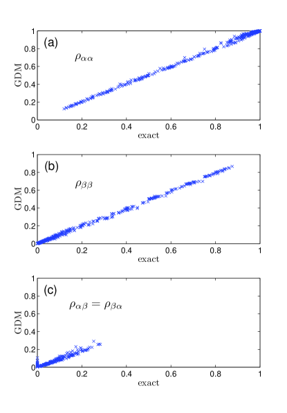
Figure 1: (Color online) Density matrix $\rho$ in the original single-particle basis for the ensemble. In panel (a) there are $360$ points corresponding to the $360$ examples in the ensemble. The horizontal coordinate of each point is $\rho_{\alpha\alpha}$ of the example by the exact diagonalization and the vertical coordinate is the one by the GDM calculation. Similarly for panels (b) and (c), but the coordinates of the points are $\rho_{\beta\beta}$ and $\rho_{\alpha\beta}$ of the examples, respectively.

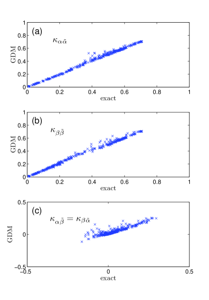
Figure 2: (Color online) Density matrix $\kappa$ in the original single-particle basis for the ensemble. In panel (a) there are $360$ points corresponding to the $360$ examples in the ensemble. The horizontal coordinate of each point is $\kappa_{\alpha\tilde{\alpha}}$ of the example by the exact diagonalization and the vertical coordinate is the one by the GDM calculation. Similarly for panels (b) and (c), but the coordinates of the points are $\kappa_{\beta\tilde{\beta}}$ and $\kappa_{\alpha\tilde{\beta}}$ of the examples, respectively.

The results for the density matrices $\rho$ and $\kappa$ in the original single-particle basis are shown in Figs. 1 and 2, respectively. Each point in these figures corresponds to one example in the ensemble with the horizontal coordinate being the exact result of the respective quantity and the vertical one being that from the GDM calculation, thus a perfect calculation would have all the points lying on the $y=x$ straight line. From Figs. 1 and 2 we see that in general the GDM theory reproduces the exact density matrices well. The root-mean-square deviations are

$$\sigma_{\rho_{\alpha\alpha}}=\sigma_{\rho_{\beta\beta}}=0.0125,~{}\sigma_{\rho_{\alpha\beta}}=\sigma_{\rho_{\beta\alpha}}=0.0198,$$

$$\sigma_{\kappa_{\alpha\tilde{\alpha}}}=0.0183,~{}\sigma_{\kappa_{\beta\tilde{\beta}}}=0.0214,~{}\sigma_{\kappa_{\alpha\tilde{\beta}}}=\sigma_{\kappa_{\beta\tilde{\alpha}}}=0.0384.$$

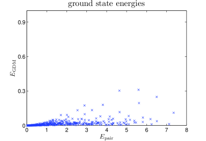
Figure 3: (Color online) Ground state energies in the ensemble. In the figure there are $360$ points corresponding to the $360$ examples in the ensemble. The horizontal coordinate of each point is the pairing correlation energy $E_{\rm{pair}}$ of the example. The vertical coordinate $E_{\rm{GDM}}$ is the ground state energy by the GDM calculation, measured from the exact ground state energy.

$\sigma_{\rho_{\alpha\alpha}}$ and $\sigma_{\rho_{\beta\beta}}$ are equal because $\rho_{\alpha\alpha}+\rho_{\beta\beta}=N/\Omega$. The results for the ground state energies are shown in Fig. 3. The horizontal coordinate of each point is the pairing correlation energy for the example $E_{\rm{pair}}\equiv\sum_{1}\epsilon_{1}n^{F}_{1}-E_{\rm{exact}}$, where $E_{\rm{exact}}$ is the exact ground state energy by the direct diagonalization, and $n^{F}_{1}=1$ or $0$ is the occupation number of the naive Fermi distribution. The vertical coordinate is the ground state energy by the GDM calculation measured from the exact one, $E_{\rm{GDM}}=\langle\phi_{N}|H|\phi_{N}\rangle-E_{\rm{exact}}$, where $\langle\phi_{N}|H|\phi_{N}\rangle$ is calculated in the canonical single-particle basis using the Hamiltonian (35) together with the recursive formulas derived in Refs. Jia_2013_1 ; Jia_arXiv_2014 . We see that in general the GDM calculation reproduces well the ground state energies: the errors are small compared with the pairing correlation energies. The average values of the errors and the pairing correlation energies for the ensemble are $\bar{E}_{\rm{GDM}}=0.0198$ and $\bar{E}_{\rm{pair}}=1.78$, respectively.

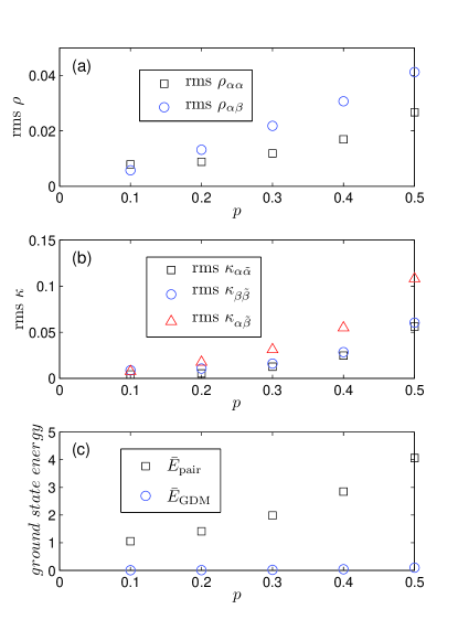
Figure 4: (Color online) Deviations of various quantities from the exact results as functions of the off-diagonal pairing strength $p$. The $360$ examples in the ensemble are divided into five subgroups according to the value of $p$. Panel (a) plots the root-mean-square deviations from the exact results of the density matrix $\rho$ by the GDM calculation within each subgroup, where black squares and blue circles are for $\rho_{\alpha\alpha}$ and $\rho_{\alpha\beta}$, respectively. Similarly panel (b) plots the root-mean-square deviations of the density matrix $\kappa$ within each subgroup, where black squares, blue circles, and red triangles are for $\kappa_{\alpha\tilde{\alpha}}$, $\kappa_{\beta\tilde{\beta}}$, and $\kappa_{\alpha\tilde{\beta}}$, respectively. In panel (c) the black squares show the average value of the pairing correlation energy $\bar{E}_{\rm{pair}}$ within each subgroup, and the blue circles show the average value of the ground state energy by the GDM calculations $\bar{E}_{\rm{GDM}}$, measured from the exact one.

At last in Fig. 4 we show the accuracy of the method depending on the off-diagonal pairing strength $p$. The $360$ examples in the ensemble are divided into five subgroups according to the value of $p$, and deviations within each subgroup of various quantities are calculated. We see that in general the errors of the GDM calculation increase with $p$. In realistic spherical nuclear shell model $p$ should be smaller than about $0.3$ based on the estimations made in the paragraph below Eq. (53). In this region the GDM theory is rather accurate.

IV Model with Zero-Range Delta Interaction

In this section we further test the theory in a semi-realistic model with the pairing Hamiltonian matrix elements calculated from the zero-range delta interaction. The model has only one species of nucleons (for example, neutrons) and the single-particle space consists of five levels: three of them ($2s_{1/2}$, $1d_{3/2}$, $1d_{5/2}$) are from the $4\hbar\omega$ major shell and two ($3s_{1/2}$, $2d_{5/2}$) are from the $6\hbar\omega$ major shell. The single-particle energies are determined by random number generator to be $\epsilon_{2s_{1/2}}=1.16$, $\epsilon_{1d_{3/2}}=2.11$, $\epsilon_{1d_{5/2}}=0.11$, $\epsilon_{3s_{1/2}}=12.98$, and $\epsilon_{2d_{5/2}}=10.37$ MeV (The gap between the $4\hbar\omega$ and $6\hbar\omega$ major shells is taken to be around $10$ MeV). The two-body pairing matrix elements [$\langle\alpha\beta;J|V|\gamma\delta;J\rangle$ with $J=0$] are calculated from the zero-range delta interaction $V(\vec{r}_{1},\vec{r}_{2})=-\lambda\delta(\vec{r}_{1}-\vec{r}_{2})$, taking the single-particle wavefunctions ($|\alpha\rangle$, $|\beta\rangle$ …) to be the harmonic oscillator ones. We perform six sets of calculations at different model parameters of the particle number $2N$ and the pairing strength $\lambda$ as listed in table 1. The unit for $\lambda$ is ${\rm{MeV}}\cdot b^{3}$, where $b=\sqrt{\hbar/(\mu\omega)}$ is the length parameter for the harmonic oscillator wavefunctions ($\mu$ is the mass of the nucleon). Values of $\lambda$ are chosen so that magnitudes of the resulting two-body pairing matrix elements are realistic. The last row of table 1 shows the average value of the pairing matrix elements of a specific form, ${\rm{mean}}[-V_{\alpha\tilde{\alpha}\tilde{\alpha}\alpha}]=-\sum_{\alpha}V_{\alpha\tilde{\alpha}\tilde{\alpha}\alpha}/(2\Omega)$, where $\alpha$ runs over the entire single-particle space whose dimension is $2\Omega$.

The results are shown in table 2. We see that in general the GDM calculation reproduces the exact density matrices accurately, except for the very small value of $\rho_{\beta\beta}$ in set5. Particularly, the abrupt change of $\kappa$ values from set3 to set4 is captured very well. The off-diagonal parts of the density matrices ($\rho_{\alpha\mu}$, $\rho_{\gamma\nu}$, $\kappa_{\alpha\tilde{\mu}}$, and $\kappa_{\gamma\tilde{\nu}}$), originating from the “off-diagonal” parts of the HFB-type pairing Hamiltonian, are always well reproduced, ranging from a less-than-one-percent effect to a few. The errors of the GDM ground state energy relative to the exact ones are shown in the last column. We see that the errors are small and consistent with the statistical estimate made within a large random ensemble for the case of a BCS-type pairing Hamiltonian in Ref. Jia_2013_2 .

V Summary

In summary, we considered the solution of the GDM pairing theory with the HFB-type Hamiltonian. In the algorithm only the one-body density matrix is computed, thus the method should be much faster than the VAPNP + HFB method in which the two-body density matrix is needed in calculating the expectation value of a two-body Hamiltonian. With the assumption that the parent and daughter nuclei were represented by pair condensates with the same pair structure, the pair-transfer amplitudes $\kappa$ could be calculated in one run together with the occupation numbers $\rho$. In contrast, the traditional variation method calculates the parent and daughter nuclei separately, each with a different pair structure.

The formalism is tested in the simple two-level model with factorizable pairing interactions, and the semi-realistic model with the zero-range delta interaction. In both cases the GDM calculation reproduces quite well the exact density matrices and ground state energy within the physical range of parameters for the realistic spherical nuclear shell model. The errors are small and consistent with the statistical estimates made within a large random ensemble for the BCS-type Hamiltonian in Ref. Jia_2013_2 . In the current form the theory is ready for the application to realistic nuclear systems.

VI Acknowledgments

Support is acknowledged from the Hujiang Foundation of China (B14004), and the startup funding for new faculty member in University of Shanghai for Science and Technology. Part of the calculations is done at the High Performance Computing Center of Michigan State University.

a

a

a

a

Table 1: Particle number $2N$ and pairing strength $\lambda$ as input parameters for the six sets of calculations. The quantity $b=\sqrt{\hbar/(\mu\omega)}$ in the unit of $\lambda$ is the length parameter for the harmonic oscillator wavefunctions. Also shown is ${\rm{mean}}[-{V}_{\alpha\tilde{\alpha}\tilde{\alpha}\alpha}]$, the average value of the pairing matrix elements of a specific form. See text for details.

	set1	set2	set3	set4	set5	set6
$N$	2	3	4	5	4	4
$\lambda/({\rm{MeV}}\cdot b^{3})$	20	20	20	20	10	40
${\rm{mean}}[-{V}_{\alpha\tilde{\alpha}\tilde{\alpha}\alpha}]/{\rm{MeV}}$	0.356	0.356	0.356	0.356	0.178	0.711

a

Table 2: Density matrices $\rho$ and $\kappa$ by the exact and GDM calculations in the original single-particle basis. For clarity each single-particle level is represented by a Greek letter as $\{\alpha,\beta,\gamma,\mu,\nu\}=\{2s_{1/2},1d_{3/2},1d_{5/2},3s_{1/2},2d_{5/2}\}$. For each set of calculation the results of density matrices $\rho$ or $\kappa$ are listed in two rows, with the top row being the exact results and the bottom row the GDM results. The last column gives the errors of the GDM ground state energy relative to the exact one, $E_{\rm{GDM}}=\langle\phi_{N}|H|\phi_{N}\rangle-E_{\rm{exact}}$.

	$\rho_{\alpha\alpha}$	$\rho_{\beta\beta}$	$\rho_{\gamma\gamma}$	$\rho_{\mu\mu}$	$\rho_{\nu\nu}$	$\rho_{\alpha\mu}$	$\rho_{\gamma\nu}$	$\kappa_{\alpha\tilde{\alpha}}$	$\kappa_{\beta\tilde{\beta}}$	$\kappa_{\gamma\tilde{\gamma}}$	$\kappa_{\mu\tilde{\mu}}$	$\kappa_{\nu\tilde{\nu}}$	$\kappa_{\alpha\tilde{\mu}}$	$\kappa_{\gamma\tilde{\nu}}$	$E_{\rm{GDM}}/{\rm{keV}}$
set1	0.0400	0.0278	0.6326	0.0007	0.0020	0.0046	0.0285	0.1972	0.1655	0.6554	0.0162	0.0275	0.0213	0.0282
	0.0536	0.0313	0.6261	0.0008	0.0016	0.0056	0.0227	0.2283	0.1760	0.6524	0.0171	0.0282	0.0224	0.0227	7.44
set2	0.0889	0.0342	0.9460	0.0009	0.0013	0.0078	0.0233	0.2910	0.1819	0.5837	0.0178	0.0265	0.0243	0.0136
	0.1086	0.0373	0.9374	0.0010	0.0011	0.0090	0.0200	0.3217	0.1919	0.5778	0.0186	0.0271	0.0253	0.0117	9.95
set3	0.9766	0.0420	0.9776	0.0030	0.0012	0.0479	0.0216	0.9418	0.1482	0.1932	0.0276	0.0163	0.0449	0.0039
	0.9423	0.0312	0.9968	0.0029	0.0007	0.0454	0.0183	0.9041	0.1762	0.2148	0.0283	0.0178	0.0423	0.0036	129
set4	0.9867	0.5254	0.9851	0.0030	0.0014	0.0478	0.0204	0.1419	0.7048	0.1455	0.0141	0.0249	0.0062	0.0024
	0.9934	0.5085	0.9947	0.0025	0.0010	0.0478	0.0189	0.1277	0.7000	0.1367	0.0138	0.0248	0.0055	0.0021	62.9
set5	0.9952	0.0078	0.9959	0.0007	0.0002	0.0231	0.0096	0.9930	0.0519	0.0576	0.0124	0.0046	0.0227	0.0005
	0.9935	0.0029	0.9999	0.0007	0.0001	0.0228	0.0089	0.9914	0.0540	0.0586	0.0127	0.0046	0.0225	0.0005	42.1
set6	0.9032	0.2134	0.8775	0.0139	0.0079	0.0990	0.0541	0.6378	0.4148	0.4880	0.0588	0.0652	0.0641	0.0255
	0.8407	0.2428	0.8795	0.0131	0.0074	0.0931	0.0471	0.5500	0.4623	0.5086	0.0587	0.0708	0.0553	0.0236	76.7

References

- (1) J. Bardeen, L. N. Cooper, and J. R. Schrieffer, Phys. Rev. 106, 162 (1957); Phys. Rev. 108, 1175 (1957).
- (2) S. T. Belyaev, K. Dan. Vidensk. Selsk. Mat. Fys. Medd. 31, (11) (1959).
- (3) A. Bohr, B. R. Mottelson, and D. Pines, Phys. Rev. 110, 936 (1958).
- (4) A. Bohr and B. Mottelson, Nuclear Structure (Benjamin, New York, 1975).
- (5) P. Ring and P. Schuck, The Nuclear Many-Body Problem (Springer-Verlag, Berlin, 1980).
- (6) K. Dietrich, H. J. Mang, and J. H. Pradal, Phys. Rev. 135, B22 (1964).
- (7) J. A. Sheikh and P. Ring, Nucl. Phys. A665, 71 (2000).
- (8) J. A. Sheikh, P. Ring, E. Lopes, and R. Rossignoli, Phys. Rev. C 66, 044318 (2002).
- (9) L. M. Robledo and G. F. Bertsch, in Fifty Years of Nuclear BCS: Pairing in Finite Systems, edited by R. A. Broglia and V. Zelevinsky (World Scientific, Singapore, 2013).
- (10) H. Flocard and N. Onishi, Annals of Physics 254, 275 (1997).
- (11) Fabian Braun and Jan von Delft, Phys. Rev. Lett. 81, 4712 (1998).
- (12) J. Dukelsky and G. Sierra, Phys. Rev. B 61, 12302 (2000).
- (13) Jan von Delft and D.C. Ralph, Physics Reports 345, 61 (2001).
- (14) M. Anguiano, J. L. Egido, and L.M. Robledo, Nucl. Phys. A696, 467 (2001).
- (15) M. Anguiano, J. L. Egido, and L.M. Robledo, Phys. Lett. B545, 62 (2002).
- (16) M. V. Stoitsov, J. Dobaczewski, R. Kirchner, W. Nazarewicz, and J. Terasaki, Phys. Rev. C 76, 014308 (2007).
- (17) J. L. Egido, P. Ring, Nucl. Phys. A383, 189 (1982); J. L. Egido, P. Ring, Nucl. Phys. A388, 19 (1982).
- (18) K. W. Schmid, F. Gruemmer, Rep. Prog. Phys. 50, 731 (1987).
- (19) L. Y. Jia, Phys. Rev. C 88, 044303 (2013).
- (20) L. Y. Jia, Phys. Rev. C 88, 064321 (2013).
- (21) S. G. Nilsson and O. Prior, Mat. Fys. Medd. Dan. Vid. Selsk 32, 16 (1961).
- (22) L. Y. Jia, arXiv:1402.1799 [nucl-th].