The approximation of almost time and band limited functions by their expansion in some orthogonal polynomials bases

Abstract.

The aim of this paper is to investigate the quality of approximation of almost time and almost band-limited functions by its expansion in three classical orthogonal polynomials bases: the Hermite, Legendre and Chebyshev bases. As a corollary, this allows us to obtain the quality of approximation in the $L^{2}-$Sobolev space by these orthogonal polynomials bases. Also, we obtain the rate of the Legendre series expansion of the prolate spheroidal wave functions. Some numerical examples are given to illustrate the different results of this work.

1. Introduction

Time-limited functions and band-limited functions play a fundamental role in signal and image processing. The time-limiting assumption is natural as a signal can only be measured over a finite duration. The band-limiting assumption is natural as well due to channel capacity limitations. It is also essential to apply sampling theory. Unfortunately, the simplest form of the uncertainty principle tells us that a signal can not be simultaneously time and band limited. A natural assumption is thus that a signal is almost time- and almost band-limited in the following sense:

Definition. Let $T,\Omega>0$ and $\varepsilon_{T},\varepsilon_{\Omega}>0$. A function $f\in L^{2}({\mathbb{R}})$ is said to be

• $\varepsilon_{T}$-almost time limited to $[-T,T]$ if

  $$\int_{|t|>T}|f(t)|^{2}\,\mathrm{d}t\leq\varepsilon_{T}^{2}{\left\|{f}\right\|}_{L^{2}({\mathbb{R}})}^{2};$$

• $\varepsilon_{\Omega}$-almost band limited to $[-\Omega,\Omega]$ if

  $$\int_{|\omega|>\Omega}|\widehat{f}(\omega)|^{2}\,\mathrm{d}\omega\leq\varepsilon_{\Omega}^{2}{\left\|{f}\right\|}_{L^{2}({\mathbb{R}})}^{2}.$$

Here and throughout this paper the Fourier transform is normalized so that, for $f\in L^{1}({\mathbb{R}})$,

$$\widehat{f}(\omega):={\mathcal{F}}[f](\omega):=\frac{1}{\sqrt{2\pi}}\int_{{\mathbb{R}}}f(t)e^{-it\omega}\,\mathrm{d}t.$$

Of course, given $f\in L^{2}({\mathbb{R}})$, for every $\varepsilon_{T},\varepsilon_{\Omega}>0$ there exist $T,\Omega>0$ such that $f$ is $\varepsilon_{T}$-almost time limited to $[-T,T]$ and $\varepsilon_{\Omega}$-almost time limited to $[-\Omega,\Omega]$. The point here is that we consider $T,\Omega,\varepsilon_{T},\varepsilon_{\Omega}$ as fixed parameters. A typical example we have in mind is that $f\in H^{s}({\mathbb{R}})$ and is time-limited to $[-T,T]$. Such an hypothesis is common in tomography, see e.g. [14], where it is required in the proof of the convergence of the filtered back-projection algorithm for approximate inversion of the Radon transform. But, if $f\in H^{s}({\mathbb{R}})$ with $s>0$, that is if

$${\left\|{f}\right\|}_{H^{s}({\mathbb{R}})}^{2}:=\int_{{\mathbb{R}}}(1+|\omega|)^{2s}|\widehat{f}(\omega)|^{2}\,\mbox{d}\omega<+\infty,$$

then

$$\int_{|\omega|>\Omega}|\widehat{f}(\omega)|^{2}\,\mbox{d}\omega \leq \int_{|\omega|>\Omega}\frac{(1+|\omega|)^{2s}}{(1+|\Omega|)^{2s}}|\widehat{f}(\omega)|^{2}\,\mbox{d}\omega$$

$$\leq \frac{{\left\|{f}\right\|}_{H^{s}({\mathbb{R}})}^{2}}{(1+|\Omega|)^{2s}}.$$

Thus $f$ is $\displaystyle\frac{1}{(1+|\Omega|)^{s}}\frac{{\left\|{f}\right\|}_{H^{s}}}{{\left\|{f}\right\|}_{L^{2}({\mathbb{R}})}}$-almost band limited to $[-\Omega,\Omega]$.

An alternative to the back projection algorithms in tomography are the Algebraic Reconstruction Techniques (that is variants of Kaczmarz algorithm, see [14]). For those algorithms to work well it is crucial to have a good representing system (basis, frame…) of the functions that one wants to reconstruct.

Thanks to the seminal work of Landau, Pollak and Slepian, the optimal orthogonal system for representing almost time and band limited functions is known. The system in questions consists of the so called prolate spheroidal wave functions, $\psi_{k}^{T}$, and has many valuable properties (see [16, 10, 11, 17, 18]). Among the most striking properties they have is that, if a function is almost time limited to $[-T,T]$ and almost band limited to $[-\Omega,\Omega]$ then it is well approximated by its projection on the first $4\Omega T$ terms of the basis:

(1.1) $$f\simeq\sum_{0\leq k<4\Omega T}{\left\langle{f,\psi_{k}^{T}}\right\rangle}\psi_{k}^{T}.$$

For more details, see [10]. This is a remarkable fact as this is exactly the heuristics given by Shannon’s sampling formula (note that to make this heuristics clearer, the functions are usually almost time-limited to $[-T/2,T/2]$ and this result is then known as the $2\Omega T$-Theorem, see [10]).

However, there is a major difficulty with prolate spheroidal wave functions that has attracted a lot of interest recently, namely the difficulty to compute them as there is no inductive nor closed form formula (see e.g. [2, 3, 4, 13, 21]). One approach is to explicitly compute the coefficients of the prolate spheroidal wave functions in terms of a basis of orthogonal polynomials like the Legendre polynomials or the Hermite functions basis. The question that then arises is that of directly approximating almost time and band limited functions by the (truncation of) their expansion in the Hermite, Legendre and Chebyshev bases. This is the question we address here.

An other motivation for this work comes from the work of the first author [8] on uncertainty principles for orthonormal bases. There, it is shown that an orthonormal basis $(e_{k})$ of $L^{2}({\mathbb{R}})$ can not have uniform time-frequency localization. Several ways of measuring localization were considered, and for most of them, the Hermite functions provided the optimal behavior. However, in one case, the proof relied on (1.1): this shows that the set of functions that are $\varepsilon_{T}$-time limited to $[-T,T]$ and $\varepsilon_{\Omega}$-band limited to $[-\Omega,\Omega]$ is almost of dimension $4\Omega T$. In particular, this set can not contain more than a fixed number of elements of an orthonormal sequence. As this proof shows, the optimal basis here consists of prolate spheroidal wave functions. As the Hermite basis is optimal for many uncertainty principles, it is thus natural to ask how far it is from optimal in this case.

Let us now be more precise and describe the main results of the paper. In Section 2, we first give a brief description of the asymptotic approximation of the Hermite functions in terms of the sine and cosine functions. Then, we use the asymptotic behaviour of the Hermite function and give an error analysis of the uniform approximation of the Hermite function projection kernel ${\displaystyle k_{n}(x,y)=\sum_{k=0}^{n}h_{k}(x)h_{k}(y)}$ by an appropriate Sinc kernel. Here, $h_{k}$ denotes the $k-$th $L^{2}$-normalized Hermite function. Then, based on the previous asymptotic approximation of the Hermite kernel, we give the quality of almost time- and band-limited functions by Hermite functions. In Section 3, we use the explicit formula for the finite Fourier transform of the Legendre polynomials in terms of the Bessel function and give the convergence rate of the Legendre series expansion of a $c-$band-limited function. Then, we extend this result to the case of almost time- and band-limited function. In Section 4, we show the results obtained for the Legendre polynomials to the case of Chebyshev polynomials. Section 5 is divided into two parts. In the first part, we first give an application of the results of Section 3 related to the convergence rate of the Legendre series expansion of the prolate spheroidal wave functions (PSWFs). Note that for a given bandwidth $c>0,$ and an integer $n\geq 0,$ the $n-$th PSWF, denoted by $\psi_{n,c}$ is a $c-$band-limited function, given as the $n-$th eigenfunction of a compact integral operator $Q_{c},$ defined on $L^{2}([-1,1])$ with the sinc kernel ${\displaystyle K_{c}(x,y)=\frac{\sin c(x-y)}{\pi(x-y)}.}$ In the second part of Section 5, we give various numerical examples that illustrate the different results of this work.

2. Approximation of almost band limited functions by Hermite functions basis.

In this section, we study the quality of approximation of band limited and almost band limited functions by the Hermite and scaled Hermite functions. For this purpose, we first need to review the asymptotic uniform approximation of the Hermite functions by the sine and cosine functions. This is the subject of the following paragraph.

2.1. Approximating Hermite functions with the WKB method.

Let $H_{n}$ be the $n$-th Hermite polynomial, that is

$$H_{n}(x)=e^{x^{2}}\frac{\mathrm{d}^{n}}{\mathrm{d}x^{n}}e^{-x^{2}}.$$

Define the Hermite functions as

$$h_{n}(x)=\alpha_{n}H_{n}(x)e^{-x^{2}/2}\quad\mbox{where }\alpha_{n}=\frac{1}{\pi^{1/4}\sqrt{2^{n}n!}}.$$

As is well known:

1. $(h_{n})_{n\geq 0}$ is an orthonormal basis of $L^{2}({\mathbb{R}})$.

2. $h_{n}$ is even if $n$ is even and odd if $n$ is odd, in particular $h_{2p}^{\prime}(0)=0$ and $h_{2p+1}(0)=0$. Further

   $$h_{2p}(0)=\frac{(-1)^{p}}{\pi^{1/4}}\sqrt{\frac{(2p-1)!!}{(2p)!!}}\quad\mbox{and}\quad h_{2p+1}^{\prime}(0)=\frac{(-1)^{p}\sqrt{4p+2}}{\pi^{1/4}}\sqrt{\frac{(2p-1)!!}{(2p)!!}}.$$

3. $h_{n}$ satisfies the differential equation $h_{n}^{\prime\prime}(x)+(2n+1-x^{2})h_{n}(x)=0$.

We will now follow the WKB method to obtain an approximation of $h_{n}$. In order to simplify notation, we will fix $n$ and drop all supscripts during the computation. Let $h=h_{n}$, $\lambda=\sqrt{2n+1}$, and define for $|x|<\lambda$

$$p(x)=\sqrt{\lambda^{2}-x^{2}},\quad\varphi(x)=\int_{0}^{x}p(t)\,\mbox{d}t\quad\mbox{and}\quad\psi_{\pm}(x)=\frac{1}{\sqrt{p(x)}}\exp\pm i\varphi(x).$$

Note that $\psi_{\pm}$ have been chosen to have

$$\psi_{+}(x)\psi_{-}^{\prime}(x)-\psi_{-}(x)\psi_{+}^{\prime}(x)=-2i$$

and

$$y^{\prime\prime}+(p^{2}-q)y=0\qquad\mbox{where }q=\frac{1}{2}\left(\frac{p^{\prime}}{p}\right)^{\prime}-\frac{1}{4}\left(\frac{p^{\prime}}{p}\right)^{2}=-\displaystyle\frac{2\lambda^{2}+3x^{2}}{4p(x)^{4}}.$$

Note that $h^{\prime\prime}(x)+p(x)h(x)=0$ so that

$$(h^{\prime}\psi_{\pm}-\psi_{\pm}^{\prime}h)^{\prime}=h^{\prime\prime}\psi_{\pm}-\psi_{\pm}^{\prime\prime}h=-qh\psi_{\pm}.$$

Let us now define

$$Q_{\pm}(x)=\int_{0}^{x}q(t)h(t)\psi_{\pm}(t)\,\mbox{d}t.$$

Integrating the previous differential equation between $0$ and $x$, we obtain the system

$$\left\{\begin{matrix}h^{\prime}(x)\psi_{+}(x)&-&h(x)\psi_{+}^{\prime}(x)&=&h^{\prime}(0)\psi_{+}(0)-h(0)\psi_{+}^{\prime}(0)&-&Q_{+}(x)\\ h^{\prime}(x)\psi_{-}(x)&-&h(x)\psi_{-}^{\prime}(x)&=&h^{\prime}(0)\psi_{-}(0)-h(0)\psi_{-}^{\prime}(0)&-&Q_{-}(x)\\ \end{matrix}\right..$$

It remains to solve this system for $h$ to obtain the principal term of $h$:

Theorem 2.1.

Let $n\geq 0$, $\lambda=\sqrt{2n+1}$. Then, for $|x|\leq\lambda$,

(2.2) $$h_{n}(x)=\sqrt{\lambda}h_{n}(0)\frac{\cos\varphi_{n}(x)}{(\lambda^{2}-x^{2})^{1/4}}+\frac{h_{n}^{\prime}(0)}{\sqrt{\lambda}}\frac{\sin\varphi_{n}(x)}{(\lambda^{2}-x^{2})^{1/4}}+E_{n}(x)$$

where

(2.3) $$\varphi_{n}(x)=\int_{0}^{x}\sqrt{\lambda^{2}-t^{2}}\,\mbox{d}t\quad\mbox{and}\quad|E_{n}(x)|\leq\frac{5}{4}\left(\frac{\lambda}{\lambda^{2}-x^{2}}\right)^{5/2}.$$

Further, if $|x|,|y|\leq T\leq\frac{\lambda}{2}$,

$$\varphi_{n}(x)=\sqrt{2n+1}x-e_{n}(x),$$

where

(2.4) $$|e_{n}(x)|\leq\frac{T^{3}}{3\lambda}\quad\mbox{and}\quad|e_{n}(x)-e_{n}(y)|\leq\frac{T^{2}}{\lambda}|x-y|,$$

while

(2.5) $$|E_{n}(x)|\leq\frac{2}{\lambda^{3}}\quad\mbox{and}\quad|E_{n}(x)-E_{n}(y)|\leq\frac{7}{\lambda^{5/2}}|x-y|.$$

Remark. One may explicitly compute $\varphi$:

$$\varphi_{n}(x)=\frac{2n+1}{2}\arcsin\frac{x}{\sqrt{2n+1}}+\frac{x}{2}\sqrt{2n+1-x^{2}}.$$

Also, $\varphi_{n}$ has a geometric interpretation: it this the area of the intersection of a disc of radius $\sqrt{2n+1}$ centered at $0$ with the strip $[0,x]\times{\mathbb{R}}^{+}$. In particular, when $x\to\sqrt{2n+1}$, $\varphi_{n}(x)\sim\frac{\pi}{4}(2n+1)$.

The result is not entirely new (e.g. [5, 6, 9, 12, 15]), except for the Lipschitz bounds of $E$. Therefore we will only sketch the proof of this theorem in Appendix A.

Using standard asymptotic of $h_{2p}(0)$ and of $h_{2p+1}^{\prime}(0)$ and the fact that $\sqrt{\lambda^{2}-x^{2}}\simeq\lambda$ when $\lambda\to\infty$, one may further simplify this result to the following:

Corollary 2.2.

Let $T\geq 2$ and let $n\geq 2T^{2}$. Then, for $|x|\leq T$, we obtain that

– if $n$ is even, $n=2p$

(2.6) $$h_{2p}(x)=\frac{(-1)^{p}}{\sqrt{\pi}p^{1/4}}\cos\varphi_{2p}(x)+\tilde{E}_{2p}(x);$$

– if $n$ is odd, $n=2p+1$

(2.7) $$h_{2p+1}(x)=\frac{(-1)^{p}}{\sqrt{\pi}p^{1/4}}\sin\varphi_{2p+1}(x)+\tilde{E}_{2p+1}(x),$$

where, for $|x|,|y|\leq T$,

(2.8) $$|\tilde{E}_{n}(x)|\leq\frac{3T^{2}}{(2n+1)^{5/4}}\quad\mbox{and}\quad|\tilde{E}_{n}(x)-\tilde{E}_{n}(y)|\leq 8\frac{T^{2}}{(2n+1)^{3/4}}|x-y|$$

To conclude, we will gather some facts about $\varphi_{n}$ that all follow from easy calculus.

Lemma 2.3.

If $|x|,|y|\leq T\leq\frac{1}{2}\sqrt{2n+1}$, then

(2.9) $$|\varphi_{n+1}(x)-\varphi_{n}(x)|\leq\frac{3T}{\sqrt{2n+1}},$$

(2.10) $$|\varphi_{n+1}(x)-\varphi_{n+1}(y)-\varphi_{n}(x)+\varphi_{n}(y)|\leq\frac{3}{\sqrt{2n+1}}|x-y|,$$

(2.11) $$|\varphi_{n+1}(x)-\varphi_{n}(x)+\varphi_{n+1}(y)-\varphi_{n}(y)|\leq\frac{5T}{\sqrt{2n+1}},$$

(2.12) $$\varphi_{n+1}(x)+\varphi_{n}(x)-\varphi_{n+1}(y)-\varphi_{n}(y)=(\sqrt{2n+1}+\sqrt{2n+3})(x-y)+\varepsilon_{n}(x,y),$$

with $\displaystyle|\varepsilon_{n}(x,y)|\leq\frac{T^{2}}{\sqrt{2n+1}}|x-y|$ and

(2.13) $$|\varphi_{n}(x)-\varphi_{n}(y)|\leq\frac{5}{4}\sqrt{2n+1}|x-y|.$$

2.2. The kernel of the projection onto the Hermite functions

As $(h_{n})_{n\geq 0}$ forms an orthonormal basis of $L^{2}({\mathbb{R}})$, every $f\in L^{2}({\mathbb{R}})$ can be written as

$$f(x)=\lim_{n\to+\infty}\sum_{k=0}^{n}{\left\langle{f,h_{k}}\right\rangle}h_{k}(x),$$

where the limit is in the $L^{2}({\mathbb{R}})$ sense. Further, for $n$ an integer, let $K_{n}f$ be the orthogonal projection of $f$ on the span of $h_{0},\ldots,h_{n}$. Then

$$K_{n}f(x)=\sum_{k=0}^{n}{\left\langle{f,h_{k}}\right\rangle}h_{k}(x)==\int_{{\mathbb{R}}}k_{n}(x,y)f(y)\,\mbox{d}y,$$

with the kernel $\displaystyle k_{n}(x,y)=\sum_{k=0}^{n}h_{k}(x)h_{k}(y)$. According to the Christoffel-Darboux Formula,

$$k_{n}(x,y)=\sqrt{\frac{n+1}{2}}\frac{h_{n+1}(x)h_{n}(y)-h_{n+1}(y)h_{n}(x)}{x-y}.$$

We will now use Corollary 2.2 to approximate this kernel:

Theorem 2.4.

Let $T\geq 2$, $n\geq 2T^{2}$ and $N=\frac{\sqrt{2n+1}+\sqrt{2n+3}}{2}$. Then, for $|x|,|y|\leq T$,

$$k_{n}(x,y)=\frac{1}{\pi}\frac{\sin N(x-y)}{x-y}+R_{n}(x,y),$$

with $|R_{n}(x,y)|\leq\displaystyle\frac{17T^{2}}{\sqrt{2n+1}}$.

Remark. The same estimate holds for $T=1$ provided $n\geq 6$. Moreover, we should mention that in practice, the actual approximation error of the kernel is much smaller than the theoretical error $R_{n}.$ See example 1 in the numerical results section that illustrate this fact.

Again, the only improvement over known results [15, 19] is in the estimate of $R_{n}$. We will therefore only sketch the proof in Appendix B.

2.3. Approximating almost time and band limited functions by Hermite functions

We can now prove the following theorem.

Theorem 2.5.

Let $\Omega_{0},T_{0}\geq 2$ and $\varepsilon_{T},\varepsilon_{\Omega}>0$. Assume that

$$\int_{|t|>T_{0}}|f(t)|^{2}\,\mathrm{d}t\leq\varepsilon_{T}^{2}{\left\|{f}\right\|}_{L^{2}({\mathbb{R}})}^{2}\quad\mbox{and}\quad\int_{|\omega|>\Omega_{0}}|\widehat{f}(\omega)|^{2}\,\mathrm{d}\omega\leq\varepsilon_{\Omega}^{2}{\left\|{f}\right\|}_{L^{2}({\mathbb{R}})}^{2}.$$

Assume that $n\geq\max(2T^{2},2\Omega^{2})$. Then, for $T\geq T_{0}$,

(2.14) $${\left\|{f-K_{n}f}\right\|}_{L^{2}([-T,T])}\leq\left(2\varepsilon_{T}+\varepsilon_{\Omega}+\frac{34T^{3}}{\sqrt{2n+1}}\right){\left\|{f}\right\|}_{L^{2}({\mathbb{R}})}$$

Proof.

We will introduce several projections. For $T,\Omega>0$, let

$$P_{T}f=\mathbf{1}_{[-T,T]}f\quad\mbox{and}\quad Q_{\Omega}f(x)={\mathcal{F}}^{-1}\bigl{[}\mathbf{1}_{[-\Omega,\Omega]}\widehat{f}](x)=\frac{1}{\pi}\int_{{\mathbb{R}}}\frac{\sin\Omega(x-y)}{x-y}f(y)\,\mbox{d}y.$$

The hypothesis on $f$ is that ${\left\|{f-P_{T}f}\right\|}_{L^{2}({\mathbb{R}})}\leq\varepsilon_{T}{\left\|{f}\right\|}_{L^{2}({\mathbb{R}})}$ for $T\geq T_{0}$ and ${\left\|{f-Q_{\Omega}f}\right\|}_{L^{2}({\mathbb{R}})}\leq\varepsilon_{\Omega}{\left\|{f}\right\|}_{L^{2}({\mathbb{R}})}$ for $\Omega\geq\Omega_{0}$. Let us also define the integral operator

$$\mathcal{R}_{n}^{T}f(x)=\int_{[-T,T]}R_{n}(x,y)f(y)\,\mbox{d}y,$$

where $R_{n}(x,y)$ are defined in Theorem 2.4. Notice that $k_{n}(x,y)=k_{n}(y,x)$ so that $R_{n}(x,y)=R_{n}(y,x)$.

It is enough to prove (2.14) for $T=T_{0}$. We may then reformulate Theorem 2.4 as following:

$$P_{T}K_{n}P_{T}f=P_{T}Q_{N}P_{T}f+P_{T}\mathcal{R}_{n}^{T}P_{T}f,$$

where $N=\frac{\sqrt{2n+1}+\sqrt{2n+3}}{2}$. Note that $N\geq\Omega_{0}$. By using (2.4), it is easy to see that

(2.15) $${\left\|{P_{T}\mathcal{R}_{n}^{T}P_{T}f}\right\|}_{L^{2}({\mathbb{R}})} \leq {\left\|{P_{T}\mathcal{R}_{n}^{T}P_{T}}\right\|}_{L^{2}({\mathbb{R}})\to L^{2}({\mathbb{R}})}{\left\|{f}\right\|}_{L^{2}({\mathbb{R}})}$$

$$\leq \|P_{T}\mathcal{R}_{n}^{T}P_{T}\|_{HS}{\left\|{f}\right\|}_{L^{2}({\mathbb{R}})}$$

$$\leq \frac{34T^{3}}{\sqrt{2n+1}}{\left\|{f}\right\|}_{L^{2}({\mathbb{R}})}.$$

Here we use the well known fact that the Hilbert-Schmidt norm of an integral operator is the $L^{2}$ norm of its kernel.

Now, using the fact that projections are contractive and $N\geq\Omega_{0}$, we have

$${\left\|{f-K_{n}f}\right\|}_{L^{2}([-T,T])} = {\left\|{P_{T}f-P_{T}K_{n}f}\right\|}_{L^{2}({\mathbb{R}})}$$

$$\leq {\left\|{P_{T}f-P_{T}K_{n}P_{T}f}\right\|}_{L^{2}({\mathbb{R}})}+{\left\|{P_{T}K_{n}(f-P_{T}f)}\right\|}_{L^{2}({\mathbb{R}})}$$

$$\leq {\left\|{P_{T}f-P_{T}Q_{N}P_{T}f+P_{T}\mathcal{R}_{n}^{T}P_{T}f}\right\|}_{L^{2}({\mathbb{R}})}+{\left\|{f-P_{T}f}\right\|}_{L^{2}({\mathbb{R}})}$$

$$\leq {\left\|{P_{T}f-P_{T}Q_{N}P_{T}f}\right\|}_{L^{2}({\mathbb{R}})}+{\left\|{P_{T}\mathcal{R}_{n}^{T}P_{T}f}\right\|}_{L^{2}({\mathbb{R}})}+{\left\|{f-P_{T}f}\right\|}_{L^{2}({\mathbb{R}})}.$$

Now, write $P_{T}Q_{N}P_{T}f=P_{T}Q_{N}f+P_{T}Q_{N}(f-P_{T}f)$, then

$${\left\|{P_{T}f-P_{T}Q_{N}P_{T}f}\right\|}_{L^{2}({\mathbb{R}})} \leq {\left\|{P_{T}f-P_{T}Q_{N}f}\right\|}_{L^{2}({\mathbb{R}})}+{\left\|{P_{T}Q_{N}(f-P_{T}f)}\right\|}_{L^{2}({\mathbb{R}})}$$

$$\leq {\left\|{f-Q_{N}f}\right\|}_{L^{2}({\mathbb{R}})}+{\left\|{f-P_{T}f}\right\|}_{L^{2}({\mathbb{R}})}.$$

Therefore,

$${\left\|{f-K_{n}f}\right\|}_{L^{2}([-T,T])} \leq {\left\|{f-Q_{N}f}\right\|}_{L^{2}({\mathbb{R}})}+\frac{34T^{3}}{\sqrt{2n+1}}{\left\|{f}\right\|}_{L^{2}({\mathbb{R}})}+2{\left\|{f-P_{T}f}\right\|}_{L^{2}({\mathbb{R}})}$$

$$\leq \left(\varepsilon_{\Omega}+\frac{34T^{3}}{\sqrt{2n+1}}+2\varepsilon_{T}\right){\left\|{f}\right\|}_{L^{2}({\mathbb{R}})},$$

since $N\geq\Omega_{0}$. ∎

Remark. The error estimate given by (2.14) is not practical due to the low decay rate of the bound of $\|\mathcal{R}_{n}^{T}\|$ given by ${\displaystyle\frac{34T^{3}}{\sqrt{2n+1}}}.$ By replacing this with a non explicit but a more realistic error estimate $\|\mathcal{R}_{n}^{T}\|_{HS},$ one gets the following error estimate which is more practical for numerical purposes,

(2.16) $${\left\|{f-K_{n}f}\right\|}_{L^{2}([-T,T])}\leq\left(\varepsilon_{\Omega}+\|\mathcal{R}_{n}^{T}\|_{HS}+2\varepsilon_{T}\right){\left\|{f}\right\|}_{L^{2}({\mathbb{R}})}.$$

2.4. Approximating almost time and band limited functions by scaled Hermite functions

For $\alpha>0$ and $f\in L^{2}({\mathbb{R}})$ we define the scaling operator $\delta_{\alpha}f(x)=\alpha^{-1/2}f(x/\alpha)$. Recall that ${\left\|{\delta_{\alpha}f}\right\|}_{L^{2}({\mathbb{R}})}={\left\|{f}\right\|}_{L^{2}({\mathbb{R}})}$ while

$${\left\|{\delta_{\alpha}f}\right\|}_{L^{2}([-A,A])}={\left\|{f}\right\|}_{L^{2}([-A/\alpha,A/\alpha A])},\ {\left\|{\delta_{\alpha}f}\right\|}_{L^{2}({\mathbb{R}}\setminus[-A,A])}={\left\|{f}\right\|}_{L^{2}({\mathbb{R}}\setminus[-A/\alpha,A/\alpha])}$$

and ${\mathcal{F}}[\delta_{\alpha}f]=\delta_{1/\alpha}{\mathcal{F}}[f]$. In particular, if $f$ is $\varepsilon_{T}$-almost time limited to $[-T,T]$ (resp. $\varepsilon_{\Omega}$-almost band limited to $[-\Omega,\Omega]$) then $\delta_{\alpha}f$ is $\varepsilon_{T}$-almost time limited to $[-T/\alpha,T/\alpha]$ (resp. $\varepsilon_{\Omega}$-almost band limited to $[-\alpha\Omega,\alpha\Omega]$).

Next, define the scaled Hermite basis $h_{k}^{\alpha}=\delta_{\alpha}h_{k}$ which is also an orthonormal basis of $L^{2}({\mathbb{R}})$ and define the corresponding orthogonal projections: for $f\in L^{2}({\mathbb{R}})$,

(2.17) $$K^{\alpha}_{n}f=\sum_{k=0}^{n}{\left\langle{f,h_{k}^{\alpha}}\right\rangle}h_{k}^{\alpha}.$$

Proposition 2.6.

Let $\alpha>0$, $T\geq 2$ and $c\geq 2/\alpha$. Assume that and

$$\int_{|t|>T}|f(t)|^{2}\,\mathrm{d}t\leq\varepsilon_{T}^{2}{\left\|{f}\right\|}_{L^{2}({\mathbb{R}})}^{2}\quad\mbox{and}\quad\int_{|\omega|>c/\alpha}|\widehat{f}(\omega)|^{2}\,\mathrm{d}\omega\leq\varepsilon_{c/\alpha}^{2}{\left\|{f}\right\|}_{L^{2}({\mathbb{R}})}^{2}.$$

Then, for $n\geq\max(2(T/\alpha)^{2},2c^{2})$, we have

(2.18) $${\left\|{f-K_{n}^{\alpha}f}\right\|}_{L^{2}([-T,T])}\leq\left(\varepsilon_{T}+\varepsilon_{c/\alpha}+\frac{34(T/\alpha)^{3}}{\sqrt{2n+1}}\right){\left\|{f}\right\|}_{L^{2}({\mathbb{R}})}.$$

Remark. The scaling with $\alpha>1$ has as effect to decrease the dependence on $T$ at the price of increasing the dependence on good frequency concentration, while taking $\alpha<1$ the gain and loss are reversed. In practice, the above dependence on $T$ is very pessimistic and $\alpha>1$ is a better choice. The most natural choice is $\alpha=T$ and $c=T\Omega$ where $\Omega$ is such that $f$ is $\varepsilon_{\Omega}$-almost band limited to $[-\Omega,\Omega]$.

Proof.

For $f\in L^{2}({\mathbb{R}})$, since $K_{n}^{\alpha}$ is contractive, we have

$${\left\|{f-K_{n}^{\alpha}f}\right\|}_{L^{2}([-T,T])} \leq {\left\|{f-K_{n}^{\alpha}P_{T}f}\right\|}_{L^{2}([-T,T])}+{\left\|{K_{n}^{\alpha}(f-P_{T}f)}\right\|}_{L^{2}([-T,T])}$$

$$\leq {\left\|{f-K_{n}^{\alpha}P_{T}f}\right\|}_{L^{2}([-T,T])}+{\left\|{f-P_{T}f}\right\|}_{L^{2}([-T,T])}$$

$$\leq {\left\|{f-K_{n}^{\alpha}P_{T}f}\right\|}_{L^{2}([-T,T])}+\varepsilon_{T}{\left\|{f}\right\|}_{L^{2}({\mathbb{R}})}.$$

Moreover,

$$K_{n}^{\alpha}P_{T}f(x) = \sum_{k=0}^{n}{\left\langle{P_{T}f,h_{k}^{\alpha}}\right\rangle}h_{k}^{\alpha}(x)=\int_{-T}^{T}f(y)\frac{1}{\alpha}\sum_{k=0}^{n}h_{k}(x/\alpha)h_{k}(y/\alpha)\,\mbox{d}y$$

$$= \int_{-T/\alpha}^{T/\alpha}f(\alpha t)\sum_{k=0}^{n}h_{k}(x/\alpha)h_{k}(t)\,\mbox{d}t.$$

From this, one easily deduces that ${\left\|{f-K_{n}^{\alpha}P_{T}f}\right\|}_{L^{2}([-T,T])}={\left\|{f_{\alpha}-K_{n}f_{\alpha}}\right\|}_{L^{2}([-\alpha T,\alpha T])}$ where $f_{\alpha}=\delta_{1/\alpha}\bigl{[}\mathbf{1}_{[-T,T]}f\bigr{]}$. Note that $f_{\alpha}$ is $0$-almost time limited to $[-T/\alpha,T/\alpha]$. Next, writing

$$\widehat{f_{\alpha}}=\delta_{\alpha}{\mathcal{F}}[\mathbf{1}_{[-T,T]}f]=\delta_{\alpha}{\mathcal{F}}[f]-\delta_{\alpha}{\mathcal{F}}[\mathbf{1}_{{\mathbb{R}}\setminus[-T,T]}f]$$

and, noting that

$${\left\|{\delta_{\alpha}{\mathcal{F}}[f]}\right\|}_{L^{2}({\mathbb{R}}\setminus[-c,c])}={\left\|{{\mathcal{F}}[f]}\right\|}_{L^{2}({\mathbb{R}}\setminus[-c/\alpha,c/\alpha])}\leq\varepsilon_{c/\alpha}{\left\|{f}\right\|}_{L^{2}({\mathbb{R}})}$$

while

$${\left\|{\delta_{\alpha}{\mathcal{F}}[\mathbf{1}_{{\mathbb{R}}\setminus[-T,T]}f]}\right\|}_{L^{2}({\mathbb{R}}\setminus[-\Omega,\Omega])} \leq {\left\|{\delta_{\alpha}{\mathcal{F}}[\mathbf{1}_{{\mathbb{R}}\setminus[-T,T]}f]}\right\|}_{L^{2}({\mathbb{R}})}$$

$$= {\left\|{\mathbf{1}_{{\mathbb{R}}\setminus[-T,T]}f}\right\|}_{L^{2}({\mathbb{R}})}\leq\varepsilon_{T}{\left\|{f}\right\|}_{L^{2}({\mathbb{R}})},$$

we get

$${\left\|{\widehat{f_{\alpha}}}\right\|}_{L^{2}({\mathbb{R}}\setminus[-c,c])}\leq\varepsilon_{c/\alpha}{\left\|{f}\right\|}_{L^{2}({\mathbb{R}})}+\varepsilon_{T}{\left\|{f}\right\|}_{L^{2}({\mathbb{R}})}.$$

It remains to apply Theorem 2.5 to complete the proof. ∎

3. Approximation of almost band limited functions in the basis of Legendre polynomials

In agreement with standard practice, we will denote by $P_{k}$ the classical Legendre polynomials, defined by the three-term recursion

$$P_{k+1}(x)=\frac{2k+1}{k+1}xP_{k}(x)-\frac{k}{k+1}P_{k-1}(x),$$

with the initial conditions

$$P_{0}(x)=1,P_{1}(x)=x.$$

These polynomials are orthogonal in $L^{2}([-1,1])$ and are normalized so that

$$P_{k}(1)=1\quad\mbox{and}\quad\int_{-1}^{1}P_{k}(x)^{2}\,\mbox{d}x=\frac{1}{k+1/2}.$$

We will denote by $\tilde{P}_{k}$ the normalized Legendre polynomial $\tilde{P}_{k}=\sqrt{k+1/2}P_{k}$ and the $\tilde{P}_{k}$’s then form an orthonormal basis of $L^{2}([-1,1])$.

In the sequel, for $c>0$, let $B_{c}$ denote the Paley-Wiener space of $c$-bandlimited functions, given by

$${\mathcal{B}}_{c}=\{f\in L^{2}(\mathbb{R});\,\,\mbox{Supp }\widehat{f}\subseteq[-c,c]\}.$$

Lemma 3.1.

Let $c>0,$ then for any $f\in{\mathcal{B}}_{c}$, and any $k\geq 0$

(3.19) $$|{\left\langle{f,P_{k}}\right\rangle}_{L^{2}(-1,1)}|\leq\frac{2}{\sqrt{2k+1}}\sqrt{\frac{e}{\pi c}}\left(\frac{ec}{2k+3}\right)^{k+1}\|f\|_{L^{2}(\mathbb{R})}.$$

Proof.

We start from the following identity relating Bessel functions of the first type to the finite Fourier transform of the Legendre polynomials, see [1]: for every $x\in{\mathbb{R}}$

(3.20) $$\int_{-1}^{1}e^{ixy}P_{k}(y)\,\mbox{d}y=2i^{k}j_{k}(x)$$

where $j_{k}$ is the spherical Bessel function defined by $j_{k}(x)=\displaystyle(-x)^{k}\left(\frac{1}{x}\frac{\mbox{d}}{\mbox{d}x}\right)^{k}\frac{\sin x}{x}$. Note that $j_{k}$ has same parity as $n$ and recall that, for $x\geq 0$, $j_{k}(x)=\displaystyle\sqrt{\frac{\pi}{2x}}J_{k+1/2}(x)$ where $J_{\alpha}$ is the Bessel function of the first kind. In particular, we have the well known bound for $x\in{\mathbb{R}}$

(3.21) $$|J_{\alpha}(x)|\leq\frac{|x|^{\alpha}}{2^{\alpha}\Gamma(\alpha+1)}\leq\frac{e^{\alpha+1}}{\sqrt{2\pi}2^{\alpha}(\alpha+1)^{\alpha+1/2}}|x|^{\alpha}$$

since $\Gamma(x)\geq\sqrt{2\pi}x^{x-1/2}e^{-x}$. From this we deduce that

(3.22) $$|j_{k}(x)|\leq\frac{e^{k+3/2}}{\sqrt{2}(2k+3)^{k+1}}|x|^{k}.$$

Now, since $f\in{\mathcal{B}}_{c}$, the Fourier inversion theorem implies that, for $x\in{\mathbb{R}}$, we have

(3.23) $$f(x)=\frac{1}{\sqrt{2\pi}}\int_{-c}^{c}\widehat{f}(\xi)e^{i\,x\,\xi}\,\mbox{d}\xi=\frac{c}{\sqrt{2\pi}}\int_{-1}^{1}\widehat{f}(c\eta)e^{i\,c\,x\,\eta}\,\mbox{d}\eta.$$

Combining (3.20) and (3.23), one gets

$${\left\langle{f,P_{k}}\right\rangle}_{L^{2}([-1,1])} = \int_{-1}^{1}f(x){P_{k}(x)}\,\mbox{d}x=\frac{c}{\sqrt{2\pi}}\int_{-1}^{1}\widehat{f}(c\eta)\left(\int_{-1}^{1}e^{-icx\eta}{P_{k}(x)}\,\mbox{d}x\right)\,\mbox{d}\eta$$

$$= i^{k}c\sqrt{\frac{2}{\pi}}\int_{-1}^{1}j_{k}(c\eta)\widehat{f}(c\eta)\,d\eta.$$

Using (3.22) together with Cauchy-Schwarz and a change of variable, one gets

$$|{\left\langle{f,P_{k}}\right\rangle}_{L^{2}([-1,1])}| \leq c^{k+1}\frac{e^{k+3/2}}{\sqrt{\pi}(2k+3)^{k+1}}\int_{-1}^{1}|\eta|^{k}|\widehat{f}(c\eta)|\,d\eta$$

$$\leq c^{k+1}\frac{e^{k+3/2}}{(2k+3)^{k+1}}\sqrt{\frac{2}{2k+1}}\sqrt{\frac{2}{\pi}}\left(\frac{1}{c}\int_{-c}^{c}|\widehat{f}(\eta)|^{2}\,d\eta\right)^{1/2}.$$

Finally, Parseval’s identity implies (3.19). ∎

Let us now introduce the following orthogonal projections on $L^{2}({\mathbb{R}})$:

$$Pf=\mathbf{1}_{(-1,1)}f,\quad Q_{c}f={\mathcal{F}}^{-1}[\mathbf{1}_{(-c,c)}{\mathcal{F}}f]\quad\mbox{and}\quad{\mathcal{L}}_{N}f=\sum_{k=0}^{N}{\left\langle{Pf,\tilde{P}_{k}}\right\rangle}\tilde{P}_{k}\mathbf{1}_{(-1,1)}.$$

Note that ${\mathcal{L}}_{N}$ is the orthogonal projection onto the subspace of $L^{2}({\mathbb{R}})$ consisting of functions of the $P(x)\mathbf{1}_{(-1,1)}$ with $P$ a polynomial of degree $\leq N$.

Theorem 3.2.

Let $c>0,$ then for any $f\in{\mathcal{B}}_{c}$, and any $N\geq\frac{ec}{2},$ we have

(3.24) $${\left\|{f-{\mathcal{L}}_{N}f}\right\|}_{L^{\infty}(-1,1)}\leq\sqrt{\frac{c}{2N+5}}\left(\frac{ec}{2N+5}\right)^{N}\|f\|_{L^{2}(\mathbb{R})}.$$

and

(3.25) $${\left\|{f-{\mathcal{L}}_{N}f}\right\|}_{L^{2}(-1,1)}\leq\sqrt{c}\left(\frac{ec}{2N+5}\right)^{N+1}\|f\|_{L^{2}(\mathbb{R})}.$$

Proof.

Note that, for $x\in(-1,1)$,

$$f(x)-{\mathcal{L}}_{N}f(x)=\sum_{k=N+1}^{+\infty}\langle f,\tilde{P}_{k}\rangle\tilde{P}_{k}(x).$$

But $\displaystyle\max\limits_{x\in(-1,1)}|\tilde{P}_{k}(x)|=|\tilde{P}_{k}(1)|=\sqrt{k+1/2}$, so that Lemma 3.1 implies

$${\left\|{f-{\mathcal{L}}_{N}f}\right\|}_{L^{\infty}(-1,1)} \leq \sum_{k=N+1}^{+\infty}(k+1/2)|\langle f,P_{k}\rangle|$$

$$\leq \sqrt{\frac{e}{\pi c}}\sum_{k=N+1}^{+\infty}\sqrt{2k+1}\left(\frac{ec}{2k+3}\right)^{k+1}\|f\|_{L^{2}(\mathbb{R})}$$

$$\leq \frac{e}{\sqrt{2N+5}}\sqrt{\frac{ec}{2\pi}}\sum_{k=N+1}^{+\infty}\left(\frac{ec}{2N+5}\right)^{k}\|f\|_{L^{2}(\mathbb{R})}$$

$$\leq \sqrt{\frac{c}{2N+5}}\left(\frac{ec}{2N+5}\right)^{N}\|f\|_{L^{2}(\mathbb{R})}.$$

If $N\geq ec/2$, we then deduce (3.24).

The proof of the $L^{2}$-bound is essentially the same:

$${\left\|{f-{\mathcal{L}}_{N}f}\right\|}_{L^{2}(-1,1)}^{2} \leq \sum_{k=N+1}^{+\infty}(k+1/2)|\langle f,P_{k}\rangle|^{2}$$

$$\leq \frac{e}{2\pi c}\sum_{k=N+1}^{+\infty}\left(\frac{ec}{2k+3}\right)^{2k+2}\|f\|_{L^{2}(\mathbb{R})}^{2}$$

$$\leq \frac{e^{2}}{2\pi}\sum_{k=N+1}^{+\infty}\left(\frac{ec}{2N+5}\right)^{2k+2}\ \|f\|_{L^{2}(\mathbb{R})}^{2}.$$

From this (3.25) easily follows when $N\geq ec/2.$ ∎

From this theorem, we simply get the following corollary:

Theorem 3.3.

Let $c>0$ and assume that $f$ is $\varepsilon_{T}$-concentrated to $(-1,1)$ and $\varepsilon_{\Omega}$-concentrated to $(-c,c)$. Then, if $N\geq ec/2$,

(3.26) $${\left\|{f-{\mathcal{L}}_{N}f}\right\|}_{L^{2}(-1,1)}\leq\left(2\varepsilon_{\Omega}+\sqrt{c}\left(\frac{ec}{2N+5}\right)^{N+1}\right){\left\|{f}\right\|}_{L^{2}({\mathbb{R}})}$$

and

(3.27) $${\left\|{f-{\mathcal{L}}_{N}f}\right\|}_{L^{2}({\mathbb{R}})}\leq\left(\varepsilon_{T}+2\varepsilon_{\Omega}+\sqrt{c}\left(\frac{ec}{2N+5}\right)^{N+1}\right){\left\|{f}\right\|}_{L^{2}({\mathbb{R}})}$$

Proof.

First

$${\left\|{f-{\mathcal{L}}_{N}f}\right\|}_{L^{2}(-1,1)} \leq {\left\|{f-Q_{c}f}\right\|}_{L^{2}(-1,1)}+{\left\|{Q_{c}f-{\mathcal{L}}_{N}Q_{c}f}\right\|}_{L^{2}(-1,1)}+{\left\|{{\mathcal{L}}_{N}(Q_{c}f-f)}\right\|}_{L^{2}(-1,1)}$$

$$\leq 2{\left\|{f-Q_{c}f}\right\|}_{L^{2}({\mathbb{R}})}+{\left\|{Q_{c}f-{\mathcal{L}}_{N}Q_{c}f}\right\|}_{L^{2}(-1,1)}.$$

But ${\left\|{f-Q_{c}f}\right\|}_{L^{2}({\mathbb{R}})}\leq\varepsilon_{\Omega}{\left\|{f}\right\|}_{L^{2}({\mathbb{R}})}$ and $Q_{c}f\in{\mathcal{B}}_{c}$ with ${\left\|{Q_{c}f}\right\|}_{L^{2}({\mathbb{R}})}\leq{\left\|{f}\right\|}_{L^{2}({\mathbb{R}})}$.

It remains to notice that

$${\left\|{f-{\mathcal{L}}_{N}f}\right\|}_{L^{2}({\mathbb{R}})}\leq{\left\|{f-P_{T}f}\right\|}_{L^{2}({\mathbb{R}})}+{\left\|{f-{\mathcal{L}}_{N}f}\right\|}_{L^{2}(-1,1)}$$

so that (3.27) follows. ∎

4. Approximation of almost band limited functions in the basis of Chebyshev polynomials

In this paragraph, we show that the basis of the Chebyshev polynomials is also well adapted for the approximation of almost band limited functions. This is essentially done by showing that the weighted finite Fourier transform of the Chebyshev polynomial is given by a formula similar to (3.20). We first recall that the classical Chebyshev polynomials $T_{k}$ are defined by the three-term recursion

$$T_{k+1}(x)=2xT_{k}(x)-T_{k-1}(x),$$

with the initial conditions

$$T_{0}(x)=1,\quad T_{1}(x)=x.$$

These polynomials are orthogonal in $L^{2}([-1,1],\,\mbox{d}\mu)$ where $\mbox{d}\mu(x)=\frac{1}{\sqrt{1-x^{2}}}\,\mbox{d}x$ and are normalized so that

(4.28) $$T_{k}(1)=1\quad\mbox{and}\quad\int_{-1}^{1}T_{n}(x)^{2}\,\mbox{d}\mu(x)=c_{k}\frac{\pi}{2}\quad\mbox{with}\quad c_{k}=\begin{cases}2&\mbox{if }k=0\\ 1&\mbox{if }k\geq 1\end{cases}$$

.

It is interesting to also note that $T_{k}(x)$ are simply given by the formula

$$T_{k}(\cos\theta)=\cos(k\theta),\quad k\in\mathbb{N},\quad\theta\in[0,\pi].$$

We will denote by $\tilde{T}_{k}$ the normalized Chebyshev polynomial $\tilde{T}_{k}=\sqrt{\frac{2}{c_{k}\pi}}T_{k}$ and the $\tilde{T}_{k}$’s then form an orthonormal basis of $L^{2}([-1,1],\,\mbox{d}\mu)$.

The following lemma gives us an explicit formula for the weighted Finite Fourier transform of $T_{k}$, that we failed to find in the literature.

Lemma 4.1.

For any $k\in\mathbb{N},$ $\widehat{T}_{k}$, the weighted finite Fourier transform of $T_{k}$ is given by

(4.29) $$\widehat{T}_{k}(x)=\int_{-1}^{1}e^{ixy}T_{k}(y)\frac{1}{\sqrt{1-y^{2}}}\,\mathrm{d}y=i^{k}\frac{\pi}{2}J_{k}(x).$$

Proof.

This results follows directly from the formula

$$\int_{-1}^{1}\frac{f(y)T_{k}(y)}{\sqrt{1-y^{2}}}\,\mathrm{d}y=\int_{0}^{\pi}f(\cos\theta)\cos k\theta\,\mbox{d}\theta$$

applied to $f(y)=e^{ixy}$ and the Poisson integral representation formula of the Bessel function. ∎

For $f\in L^{2}([-1,1],\mbox{d}\mu)$ we now define

$${\mathcal{T}}_{n}f=\sum_{k=0}^{n}{\left\langle{f,\tilde{T}_{k}}\right\rangle}\tilde{T}_{k}$$

the projection of $f$ on ${\mathbb{C}}_{n}[X]$ the subspace of $L^{2}([-1,1],\mbox{d}\mu)$ consisting of polynomials of degree $\leq n$. We can now prove the Chebyshev version of Lemma 3.1 and the approximation rate of band-limited functions by their projection on the Chebyshev orthonomal basis in $L^{2}([-1,1]\,\mbox{d}\mu)$. However, note that an $L^{2}({\mathbb{R}})$ function restricted to $[-1,1]$ need not be in $L^{2}([-1,1]\,\mbox{d}\mu)$. Therefore, its expansion in the Chebyshev system need not converge (and not even be defined). Thus, we cannot extend Theorem 3.3 to the Chebyshev setting.

Proposition 4.2.

Let $c>0,$ then for any $f\in{\mathcal{B}}_{c}$, and any $k\geq 0$

(4.30) $$|{\left\langle{f,T_{k}}\right\rangle}_{L^{2}([-1,1],\mbox{d}\mu)}|\leq\frac{1}{\sqrt{(2k+1)c}}\left(\frac{ec}{2(k+1)}\right)^{k+1}\|f\|_{L^{2}(\mathbb{R})},$$

and, if $N\geq ec/2$,

$${\left\|{f-{\mathcal{T}}_{N}f}\right\|}_{L^{2}([-1,1],\mathrm{d}\mu)}\leq\frac{e\sqrt{c}}{2(2N+3)}\left(\frac{ce}{2N+4}\right)^{N+1}\|f\|_{L^{2}(\mathbb{R})}^{2}.$$

Proof.

Since $f\in{\mathcal{B}}_{c}$, then the Fourier inversion theorem implies that, for $x\in{\mathbb{R}}$, we have

$$f(x)=\frac{1}{\sqrt{2\pi}}\int_{-c}^{c}\widehat{f}(\xi)e^{i\,x\,\xi}\,\mbox{d}\xi=\frac{c}{\sqrt{2\pi}}\int_{-1}^{1}\widehat{f}(c\eta)e^{i\,c\,x\,\eta}\,\mbox{d}\eta.$$

Combining this with (3.20), one gets

$${\left\langle{f,T_{k}}\right\rangle}_{L^{2}([-1,1],\mbox{d}\mu)} = \int_{-1}^{1}f(x)\overline{T_{k}(x)}\,\frac{\mbox{d}x}{\sqrt{1-x^{2}}}$$

$$= \frac{c}{\sqrt{2\pi}}\int_{-1}^{1}\widehat{f}(c\eta)\left(\int_{-1}^{1}e^{-icx\eta}\overline{T_{k}(x)}\,\frac{\mbox{d}x}{\sqrt{1-x^{2}}}\right)\,\mbox{d}\eta$$

$$= i^{k}\frac{c\sqrt{2\pi}}{4}\int_{-1}^{1}\frac{\pi}{2}J_{k}(x)(c\eta)\widehat{f}(c\eta)\,d\eta.$$

Using (3.21) together with Cauchy-Schwarz inequality and a change of variable, one gets

$$|{\left\langle{f,T_{k}}\right\rangle}_{L^{2}([-1,1])}| \leq c^{k+1}\frac{e^{k+1}}{2^{k+2}(k+1)^{k+1/2}}\int_{-1}^{1}|\eta|^{k}|\widehat{f}(c\eta)|\,d\eta$$

$$\leq c^{k+1/2}\frac{e^{k+1}}{2^{k+3/2}(k+1)^{k+1}}\sqrt{\frac{2}{2k+1}}\left(\int_{-c}^{c}|\widehat{f}(\eta)|^{2}\,d\eta\right)^{1/2}$$

To conclude, it suffices to use Parseval’s identity.

From the orthonormality of the $\tilde{T}_{k}$’s and this bound, we deduce that

$${\left\|{f-{\mathcal{T}}_{N}f}\right\|}_{L^{2}([-1,1],\mbox{d}\mu)}^{2} \leq \sum_{k=N+1}^{+\infty}|\langle f,\tilde{T}_{k}\rangle_{L^{2}([-1,1],\mbox{d}\mu)}|^{2}$$

$$\leq \sum_{k=N+1}^{+\infty}\frac{1}{2k+1}c^{2k+1}\frac{e^{2k+2}}{2^{2k+3}(k+1)^{2k+2}}\|f\|_{L^{2}(\mathbb{R})}^{2}$$

$$\leq \frac{1}{2N+3}\frac{e}{2N+4}\sum_{k=N+1}^{+\infty}\left(\frac{ce}{2(k+1)}\right)^{2k+1}\|f\|_{L^{2}(\mathbb{R})}^{2}$$

$$\leq \frac{e^{2}c}{4}\frac{1}{(2N+3)^{2}}\left(\frac{ec}{2N+4}\right)^{2N+4}\|f\|_{L^{2}(\mathbb{R})}^{2}$$

provided $N\geq ec/2$. ∎

5. Applications and numerical results

In the first part of this last section, we apply the quality of approximation of $c-$bandlimited functions by Legendre polynomials in the framework of prolate spheroidal wave functions (PSWFs). As a consequence, we give the convergence rate of the Flammer’s scheme, see [7] for the computation of the PSWFs.

5.1. Approximation of prolate spheroidal wave functions

For a given real number $c>0,$ called bandwidth, the Prolate spheroidal wave functions (PSWFs) denoted by $(\psi_{n,c}(\cdot))_{n\geq 0}$, are defined as the bounded eigenfunctions of the Sturm-Liouville differential operator $\mathcal{L}_{c},$ defined on $C^{2}([-1,1]),$ by

(5.31) $$\mathcal{L}_{c}(\psi)=-(1-x^{2})\frac{d^{2}\psi}{d\,x^{2}}+2x\frac{d\psi}{d\,x}+c^{2}x^{2}\psi.$$

They are also the eigenfunctions of the finite Fourier transform $\mathcal{F}_{c}$, as well as the ones of the operator $\displaystyle\mathcal{Q}_{c}=\frac{c}{2\pi}\mathcal{F}^{*}_{c}\mathcal{F}_{c},$ which are defined on $L^{2}([-1,1])$ by

(5.32) $$\mathcal{F}_{c}(f)(x)=\int_{-1}^{1}e^{i\,c\,x\,y}f(y)\,\mbox{d}y,\quad\mbox{and}\quad\mathcal{Q}_{c}(f)(x)=\int_{-1}^{1}\frac{\sin(c(x-y))}{\pi(x-y)}f(y)\,\mbox{d}y.$$

They are normalized so that their $L^{2}([-1,1])$ norm is equal to $1$ and $\psi_{n,c}(1)>0$. We call $(\chi_{n}(c))_{n\geq 0}$ the corresponding eigenvalues of $\mathcal{L}_{c}$, $\mu_{n}(c)$ the eigenvalues of $\mathcal{F}_{c}$ and $\lambda_{n}(c)$ the ones of $\mathcal{Q}_{c}$. A well known property is then that ${\left\|{\psi_{n,c}}\right\|}_{L^{2}({\mathbb{R}})}=\frac{1}{\sqrt{\lambda_{n}(c)}}$.

The crucial commuting property of $\mathcal{L}_{c}$ and $Q_{c}$ has been first observed by Slepian and co-authors [16], whose name is closely associated to all properties of PSWFs and their associated spectrum. Among their basic properties we cite their analytic extension to the whole real line and their unique properties to form an orthonormal basis of $L^{2}([-1,1])$ and an orthonormal basis of ${\mathbb{B}}_{c}$. A well known estimate for $\chi_{n}(c)$ is

(5.33) $$n(n+1)\leq\chi_{n}(c)\leq n(n+1)+c^{2}.$$

Recall that $\lambda_{n}(c)$ and $\mu_{n}(c)$ are related by $\lambda_{n}(c)=\displaystyle\frac{c}{2\pi}|\mu_{n}(c)|^{2}$. A precise asymptotic of $\lambda_{n}(c)$ has been established by Widom [20]. Recently in [3], the authors have given an explicit approximation of the $\lambda_{n}(c),$ valid for $n>2c/\pi$ that gives rise to the exact super-exponential decay rate of the sequence of these eigenvalues. But, here we want a lower bound that is valid for all $n$. According to [11],

(5.34) $$0<\lambda_{n}(c)<1\quad\mbox{and}\quad\lambda_{{\left[{\frac{2}{\pi}c}\right]}+1}<\frac{1}{2}<\lambda_{{\left[{\frac{2}{\pi}c}\right]}-1}$$

while Bonami-Karoui established the following bound, see [2]

(5.35) $$\lambda_{n}(c)\geq\frac{2}{5}\left(\frac{2c}{\pi(n+1)}\right)^{5(n+1)}\quad\mbox{for }n\geq\max\left(3,\frac{2}{\pi}c\right).$$

In Appendix C we will prove the following slight improvement of this bound:

Proposition 5.1.

Let $c$ be a real number. Then, if $\displaystyle n>\frac{2}{\pi}c$,

$$\lambda_{n}(c)\geq 7\left(1-\frac{2c}{n\pi}\right)^{2}\left(\frac{c}{7\pi n}\right)^{2n-1}.$$

If $\displaystyle n={\left[{\frac{2}{\pi}c}\right]}$, $\lambda_{n}(c)\geq\displaystyle\frac{4}{\pi+2c}$.

Since $\psi_{n,c}\in L^{2}([-1,1])$, we may expand it in the Legendre basis

$$\psi_{n,c}=\sum_{k=0}^{+\infty}{\left\langle{\psi_{n,c},\tilde{P}_{k}}\right\rangle}\tilde{P}_{k}=\sum_{k=0}^{+\infty}\left(k+\frac{1}{2}\right){\left\langle{\psi_{n,c},P_{k}}\right\rangle}P_{k}.$$

Notation : Let us write $\beta_{k}^{n}(c)=\left(k+\frac{1}{2}\right){\left\langle{\psi_{n,c},P_{k}}\right\rangle}$ so that, on $[-1,1]$,

(5.36) $$\psi_{n,c}=\sum_{k=0}^{+\infty}\beta_{k}^{n}(c)P_{k}.$$

Rokhlin, Xiao and Yarvin [21] have obtained induction formulas for the $\beta_{k}^{n}(c)$’s in order to compute the $\psi_{n,c}$’s. Let us now obtain an estimate for them:

Corollary 5.2.

With the above notation, we have

$$|\beta_{k}^{n}(c)|\leq\begin{cases}2\sqrt{\frac{e}{\pi c}}{\sqrt{2k+1}}\left(\frac{ec}{2k+3}\right)^{k+1}&\mbox{if }n\leq{\left[{\frac{2}{\pi}c}\right]}-1\\ \sqrt{\frac{e(\pi+2c)}{2\pi c}}{\sqrt{k+1/2}}\left(\frac{ec}{2k+3}\right)^{k+1}&\mbox{if }n={\left[{\frac{2}{\pi}c}\right]}\\ \sqrt{\frac{2e}{7\pi}}\frac{1}{\sqrt{c}}\left(1-\frac{2c}{n\pi}\right)^{-1}\left(\frac{7\pi n}{c}\right)^{n-1/2}{\sqrt{k+1/2}}\left(\frac{ec}{2k+3}\right)^{k+1}&\mbox{if }n\geq{\left[{\frac{2}{\pi}c}\right]}+1\end{cases}.$$

Proof.

Since $\psi_{n,c}\in{\mathcal{B}}_{c}({\mathbb{R}})$, from Lemma 3.1 we deduce that

$$|{\left\langle{\psi_{n,c},P_{k}}\right\rangle}|\leq 2\sqrt{\frac{e}{\pi c}}\frac{1}{\sqrt{2k+1}}\left(\frac{ec}{2k+3}\right)^{k+1}\|\psi_{n,c}\|_{L^{2}(\mathbb{R})}=2\sqrt{\frac{e}{\pi c}}\frac{1}{\sqrt{2k+1}}\left(\frac{ec}{2k+3}\right)^{k+1}\frac{1}{\sqrt{\lambda_{n}(c)}}$$

To conclude, it suffices to use the lower bounds of $\lambda_{n}(c)$ given by (5.34) and the previous proposition. ∎

From this, one can then easily obtain error estimates for the approximation of prolate spheroidal wave functions by the truncation of their expansion in the Legendre basis in the spirit of Theorem 3.3.

5.2. Numerical results

In this paragraph, we give several examples that illustrate the different results of this work.

Example 1. In this example, we check numerically that the actual error of the uniform approximation of the kernel ${\displaystyle k_{n}(x,y)=\sum_{k=0}^{n}h_{k}(x)h_{k}(y)}$ may be much smaller than the theoretical error given by Theorem 2.4. For this purpose, we have considered the value $T=1$ and various values of the integer $10\leq n\leq 100$. For each value of $n$, we have used a uniform discretization $\Lambda$ of the square $[-1,1]^{2}$ with equidistant 6400 nodes. Then, we have computed over these grid points, a highly accurate approximation ${\displaystyle\widetilde{E}_{n}=\sup_{x,y\in\Lambda}\left|k_{n}(x,y)-\frac{\sin N(x-y)}{\pi(x-y)}\right|}$ of the exact uniform error ${\displaystyle E_{n}=\sup_{x,y\in[-1,1]}\left|k_{n}(x,y)-\frac{\sin N(x-y)}{\pi(x-y)}\right|}$. The obtained results are given by Table 1.

$n$	10	25	50	75	100
$\widetilde{E}_{n}$	0.067	0.039	0.025	0.023	0.022

Table 1. Approximate errors $\widetilde{E}_{n}$ for various values of $n$.

Example 2. In this example, we illustrate the quality of approximation by scaled Hermite functions of a time-limited and an almost band-limited function. For this purpose, we consider the function $f(x)=1_{[-1/2,1/2]}(x)$. From the Fourier transform of $f$, one can easily check that $f\in H^{s}(\mathbb{R})$ for any $s<1/2$. Note that $f$ is $0$-concentrated in $[-1/2,1/2]$ and since $f\in H^{s}(\mathbb{R})$, $f$ is $\epsilon_{\Omega}$-band concentrated in $[-\Omega,+\Omega]$, with $\epsilon_{\Omega}<M_{s}\Omega^{-s}$ with $M_{s}$ a positive constant. We have considered the value of $c=100$ and we have used (2.17) to compute the scaled Hermite approximations $K_{n}^{c}(f)$ of $f$ with $n=40$ and $n=80$. The graphs of $f$ and its scaled Hermite approximation are given by Figure 1. In Figure 2, we have given the approximation errors $f(x)-K_{n}^{c}f(x).$
Also, to illustrate the fact that the scaled Hermite approximation outperforms the usual Hermite approximation, we have repeated the previous numerical tests without the scaling factor (this corresponds to the special case of $c=1$). Figure 3 shows the graphs of $f$ and $K_{n}f$. This clearly illustrates the out-performance of the scaled Hermite approximation, compared to the usual Hermite approximation.

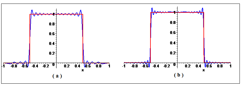
Figure 1. Graph of the approximation of $f(x)$ (red) by $K_{n}^{c}f(x)$, $c=100$ (blue) with (a) $n=40$ (b) $n=80$.

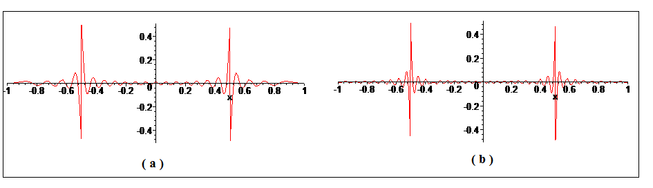
Figure 2. Graph of the approximation error $f(x)-K_{n}^{c}f(x)$, $c=100$ with (a) $n=40$ (b) $n=80$.

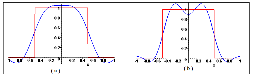
Figure 3. Graph of the approximation of $f(x)$ (red) by $K_{n}^{c}f(x)$, $c=1$ (blue) with (a) $n=40$ (b) $n=80$.

Example 3. In this example, we illustrate the decay rate of the Legendre and Chebyshev expansion coefficients of a $c$-bandlimited functions, that we have given by (3.19) and (4.30), respectively. For this purpose, we have considered the function $f\in B_{c},$ given by ${\displaystyle f_{c}(x)=\frac{\sin(cx)}{cx},\,x\in\mathbb{R}}$. Then, we have computed the different Legendre and Chebyshev expansion coefficients $l_{n}(f)={\left\langle{f,\overline{P_{n}}}\right\rangle}_{L^{2}(I)}$ and $c_{n}(f)={\left\langle{f,\overline{T_{n}}}\right\rangle}_{L^{2}(I,d\mu)}$of $f_{c},$ for the two values of $c=10$ and $c=50$. In Figure 4, we plot the graphs of the $\log(|l_{n}(f)|),\,\log(|c_{n}(f)|),\,n\geq\left[\frac{ec}{2}\right]+1$ versus the logarithm of their respective error bounds given by (3.19) and (4.30).

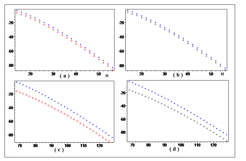
Figure 4. (a) graph of $\log(|l_{n}(f_{c})|)$, $c=10$ (in red) versus the logarithm of its bound (3.19) (in blue), (b) graph of $\log(|c_{n}(f_{c})|)$, $c=10$ (in black) versus the logarithm of its bound (4.30) (in blue); (c) and (d) same as in (a) and (b) with $c=50$.

Example 4. In this last example, we illustrate the quality of approximation by Legendre and Chebyshev polynomials in the Sobolev spaces $H^{s}(I).$ We have considered the two functions $f,g$ given by $f(x)=1_{[-1/2,1/2]}(x)$ and $g(x)=(1-|x|)1_{[-1,1]}(x).$ It is clear that $g\in H^{s}(I),\,\forall s<3/2.$ In Figure 5, we plot the graphs of the approximation error of $f$ by its corresponding projections $\mathcal{L}_{N}f$ and $\mathcal{T}_{N}f$ over the subspaces spanned by the first $N+1$ Legendre and Chebyshev polynomials, respectively, with $N=50.$ In Figure 6, we plot the graphs of $g-\mathcal{L}_{N}g$ and $g-\mathcal{T}_{N}g$ with $N=50$.

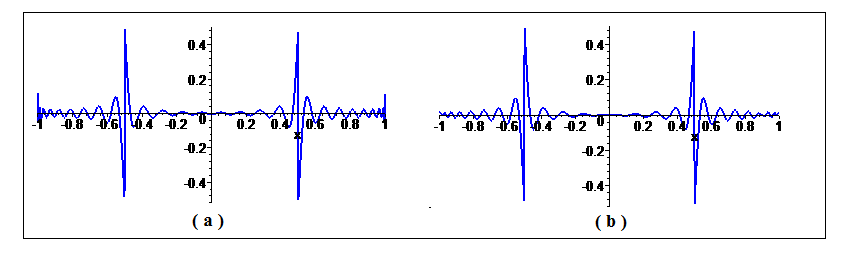
Figure 5. (a) Graphs of the errors $f(x)-\mathcal{L}_{N}f(x),$ with $N=50$ (b) same as (a) with $f(x)-\mathcal{T}_{N}f(x),$.

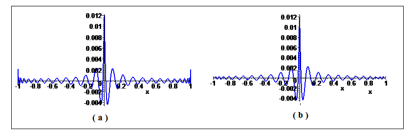
Figure 6. (a) Graphs of the errors $g(x)-\mathcal{L}_{N}g(x),$ with $N=50$ (b) same as (a) with $g(x)-\mathcal{T}_{N}g(x),$.

Appendix A Proof of Theorem 2.1

.

We will again drop the index $n$ and use the notation introduced before the statement of the theorem.

The bounds for $e(x)$ are obtained by standard calculus, we will thus omit the proof. As for $E(x)$, the computation shows

$$E(x)=\frac{1}{\sqrt{p(x)}}\int_{0}^{x}\frac{q(t)}{\sqrt{p(t)}}h(t)\sin\bigl{(}\varphi(x)-\varphi(t)\bigr{)}\,\mbox{d}t.$$

Using Cauchy-Schwarz, we obtain

$$|E(x)|\leq\frac{1}{\sqrt{p(x)}}\left(\int_{0}^{x}\frac{q(t)^{2}}{p(t)}\,\mbox{d}t\right)^{1/2}\left(\int_{0}^{x}h(t)^{2}\,\mbox{d}t\right)^{1/2}\leq\frac{1}{\sqrt{p(x)}}\left(\int_{0}^{x}\frac{25\lambda^{4}}{16p(t)^{9}}\,\mbox{d}t\right)^{1/2}$$

since ${\left\|{h_{n}}\right\|}_{2}=1$. As $|x|<\lambda$, and $p$ decreases, the estime $|E(x)|\leq\displaystyle\frac{5\lambda^{5/2}}{4p(x)^{5}}$ follows. When $|x|\leq\lambda/2$, the change of variable $y=\lambda s$ and a numerical computation shows that $|E(x)|\leq\frac{2}{\lambda^{3}}$.

Note that this bound on $E$ directly leads to a bound on $h$. For instance, if $n\geq 2$ is even, then $|h_{2n}(x)|\leq\displaystyle\frac{1}{\sqrt{p(x)}}$ for $|x|\leq\lambda/2$.

The Lipschitz bound on $E$ is a bit more subtle so let us give more details. First, we introduce some further notation:

$$\chi(x,t)=\frac{q(t)}{\sqrt{p(t)}}h(t)\sin\bigl{(}\varphi(x)-\varphi(t)\bigr{)}\quad\mbox{and}\quad\Phi(x,y)=\int_{0}^{x}\chi(y,t)\,\mbox{d}t.$$

Now, write

$$E(y)-E(x) = \left(\frac{1}{\sqrt{p(y)}}-\frac{1}{\sqrt{p(x)}}\right)\Phi(y,y)+\frac{1}{\sqrt{p(x)}}\bigl{[}\Phi(y,y)-\Phi(x,y)\bigr{]}$$

$$\frac{1}{\sqrt{p(x)}}\bigl{[}\Phi(x,y)-\Phi(x,x)\bigr{]}=E_{1}+E_{2}+E_{3}.$$

We have proved that for $|y|<\lambda/2$, $\Phi(y,y)\leq 2\lambda^{-3}$. Simple calculus then implies that $|E_{1}|\leq\displaystyle\frac{|x-y|}{\lambda^{9/2}}$ when $|x|,|y|<\lambda/2$.

Next, if $|x|,|y|\leq(1-\eta)\lambda$ one can estimate $E_{2}$ as follows:

$$|\Phi(y,y)-\Phi(x,y)| \leq \int_{x}^{y}|\chi(y,t)|\,\mbox{d}t\leq|x-y|\sup_{|t|\leq\lambda/2}\frac{q(t)}{\sqrt{p(t)}}\sup_{|t|\leq\lambda/2}|h(t)|$$

$$\leq \frac{5\lambda^{2}}{4p(y)^{5}}|x-y|.$$

Therefore, $|E_{2}|\leq\displaystyle\frac{3}{\lambda^{7/2}}|x-y|$.

Finally,

$$\Phi(x,y)-\Phi(x,x) = \int_{0}^{x}\frac{q(t)}{\sqrt{p(t)}}h(t)\Bigl{[}\sin\bigl{(}\varphi(y)-\varphi(t)\bigr{)}-\sin\bigl{(}\varphi(x)-\varphi(t)\bigr{)}\Bigr{]}\,\mbox{d}t$$

$$= 2\int_{0}^{x}\frac{q(t)}{\sqrt{p(t)}}h(t)\cos\frac{\varphi(x)+\varphi(y)-2\varphi(t)}{2}\,\mbox{d}t\sin\frac{\varphi(y)-\varphi(x)}{2}.$$

The integral is estimated in the same way as we estimated $\Phi(x,x)$, while for $\varphi$ we use the mean value theorem and the fact that $\varphi^{\prime}=p$. We, thus, get $|E_{3}|\leq\displaystyle\frac{2}{\lambda^{5/2}}|x-y|$. The estimate for $E$ follows.

Appendix B Proof of Theorem 2.4

.

For sake of simplicity, we will only prove the theorem in the case when $n$ is even and write $n=2p$. Let $\lambda=\sqrt{2n+1}$, $\mu=\sqrt{2n+3}$, $\alpha=\frac{1}{\sqrt{\pi}p^{1/4}}$, $\beta=\frac{1}{\sqrt{\pi}p^{1/4}}$, $E=(-1)^{p}\tilde{E}_{2p}$ and $F=(-1)^{p}\tilde{E}_{2p+1}$. Then, according to Corollary 2.2

$$\left\{\begin{matrix}h_{2p}(x)&=&(-1)^{p}\bigl{(}\frac{1}{\sqrt{\pi}p^{1/4}}\cos\varphi_{2p}(x)+E(x)\bigr{)}\\ h_{2p+1}(x)&=&(-1)^{p}\bigl{(}\frac{1}{\sqrt{\pi}p^{1/4}}\sin\varphi_{2p+1}(x)+F(x)\bigr{)}\end{matrix}\right..$$

Therefore, $h_{2p+1}(x)h_{2p}(y)-h_{2p+1}(y)h_{2p}(x)$ is

$$= \frac{1}{\pi p^{1/2}}\bigl{(}\sin\varphi_{2p+1}(x)\cos\varphi_{2p}(y)-\sin\varphi_{2p+1}(y)\cos\varphi_{2p}(x)\bigr{)}$$

$$+\frac{1}{\sqrt{\pi}p^{1/4}}\bigl{(}F(x)\cos\varphi_{2p}(y)-F(y)\cos\varphi_{2p}(x)\bigr{)}$$

$$+\frac{1}{\sqrt{\pi}p^{1/4}}\bigl{(}\sin\varphi_{2p+1}(x)E(y)-\sin\varphi_{2p+1}(y)E(x)\bigr{)}$$

$$+F(x)E(y)-F(y)E(x).$$

The last three terms are all of the form

$$A(x)B(y)-B(x)A(y)=\bigl{(}A(x)-A(y)\bigr{)}B(y)+\bigl{(}B(y)-B(x)\bigr{)}A(y)$$

and are thus bounded with the help of the uniform and Lipschitz bounds of $A$ and $B$ by a factor of $|x-y|$.

The first term is the principal one. Let us start by computing

$$C:=\sin\varphi_{2p+1}(x)\cos\varphi_{2p}(y) - \sin\varphi_{2p+1}(y)\cos\varphi_{2p}(x)$$

$$= \frac{1}{2}\bigl{[}\sin\bigl{(}\varphi_{2p+1}(x)+\varphi_{2p}(y)\bigr{)}-\sin\bigl{(}\varphi_{2p+1}(x)-\varphi_{2p}(y)\bigr{)}$$

$$\qquad-\sin\bigl{(}\varphi_{2p+1}(y)+\varphi_{2p}(x)\bigr{)}+\sin\bigl{(}\varphi_{2p+1}(y)-\varphi_{2p}(x)\bigr{)}\bigr{]}$$

$$= \sin\frac{\varphi_{2p+1}(x)-\varphi_{2p+1}(y)-\varphi_{2p}(x)+\varphi_{2p}(y)}{2}$$

$$\times\cos\frac{\varphi_{2p+1}(x)+\varphi_{2p+1}(y)+\varphi_{2p}(x)+\varphi_{2p}(y)}{2}$$

$$+\sin\frac{\varphi_{2p+1}(y)+\varphi_{2p}(y)-\varphi_{2p}(x)-\varphi_{2p+1}(x)}{2}$$

$$\times\cos\frac{\varphi_{2p+1}(x)-\varphi_{2p}(x)-\varphi_{2p}(y)+\varphi_{2p+1}(y)}{2}$$

$$= S_{1}C_{1}+S_{2}(C_{2}-1)+S_{2}.$$

Now, according to (2.10),

$$|S_{1}C_{1}|\leq|S_{1}|\leq\frac{|\varphi_{2p+1}(x)-\varphi_{2p+1}(y)-\varphi_{2p}(x)+\varphi_{2p}(y)|}{2}\leq\frac{3}{2\sqrt{2n+1}}|x-y|.$$

With (2.11),

$$|C_{2}-1|\leq\frac{|\varphi_{2p+1}(x)-\varphi_{2p}(x)-\varphi_{2p}(y)+\varphi_{2p+1}(y)|^{2}}{2}\leq\frac{25T^{2}}{2(2n+1)}.$$

Thus, with (2.12),

$$|S_{2}(C_{2}-1)|\leq\left(N+\frac{T^{2}}{\sqrt{2n+1}}\right)|x-y|\frac{25T^{2}}{2(2n+1)}\leq\frac{16T^{2}}{\sqrt{2n+1}}|x-y|.$$

Finally, using again Lemma 2.3, $\sin\bigl{(}N(y-x)+\varepsilon_{n}(y,x)\bigr{)}$ is

$$= \sin N(y-x)+\sin N(y-x)\bigl{(}\cos\varepsilon_{n}(y,x)-1\bigr{)}+\cos N(y-x)\sin\varepsilon_{n}(x,y)$$

$$= \sin N(y-x)+E_{2}(x,y),$$

where

$$|E_{2}(x,y)|\leq|\varepsilon_{n}(x,y)|+\frac{|\varepsilon_{n}(x,y)|^{2}}{2}\leq\frac{2T^{2}}{\sqrt{2n+1}}|x-y|.$$

It remains to group all estimates to get the result.

Appendix C Proof of Proposition 5.1

.

Recall that we want to prove that, if $\displaystyle n>\frac{2}{\pi}c$,

$$\lambda_{n}(c)\geq 7\left(1-\frac{2c}{n\pi}\right)^{2}\left(\frac{c}{7\pi n}\right)^{2n-1}.$$

If $\displaystyle n={\left[{\frac{2}{\pi}c}\right]}$, $\lambda_{n}(c)\geq\displaystyle\frac{4}{\pi+2c}$.

According to the min-max Theorem, for any $n$-dimensional subspace $V$ of $L^{2}({\mathbb{R}})$

$$\lambda_{n}(c)\geq\min_{f\in V\setminus\{0\}}\frac{{\left\langle{\mathcal{Q}_{c}f,f}\right\rangle}_{L^{2}({\mathbb{R}})}}{{\left\|{f}\right\|}_{L^{2}({\mathbb{R}})}^{2}}.$$

To show the theorem, we consider $V$ to be the space of functions that is constant on each interval of the form

$$I_{j}:=\left(-1+\frac{2j}{n},-1+\frac{2j+2}{n}\right),\quad j=0,\ldots,n-1.$$

Take $f\in V$ and write $\displaystyle f=\sum_{j=0}^{n-1}f_{j}\chi_{I_{j}}$. Then

$${\left\|{f}\right\|}_{2}^{2}=\displaystyle\frac{2}{n}\sum_{j=0}^{n-1}|f_{j}|^{2}.$$

On the other hand, write

$$\widehat{f}(\omega):={\mathcal{F}}[f](\omega):=\frac{1}{\sqrt{2\pi}}\int_{{\mathbb{R}}}f(t)e^{-it\omega}\,\mathrm{d}t$$

for the Fourier transform and note that $\mathcal{Q}_{c}(f)=\mathcal{F}^{-1}\bigl{(}\mathbf{1}_{[-c,c]}\mathcal{F}\bigr{)}$. Parseval’s Identity shows that

$${\left\langle{\mathcal{Q}_{c}f,f}\right\rangle}_{L^{2}({\mathbb{R}})}=\int_{-c}^{c}|\widehat{f}|^{2}\,d\xi.$$

But

$$\widehat{f}(\xi) = \frac{1}{\sqrt{2\pi}}\int_{-1}^{1}f(t)e^{-i\xi t}\,\mathrm{d}t=\frac{1}{\sqrt{2\pi}}\sum_{j=0}^{n-1}f_{j}\int_{-1+\frac{2j}{n}}^{-1+\frac{2j+2}{n}}e^{-i\xi t}\,\mathrm{d}t$$

$$= \frac{1}{\sqrt{2\pi}}\sum_{j=0}^{n-1}f_{j}e^{-i\xi\left(-1+\frac{2j+1}{n}\right)}\int_{-\frac{1}{n}}^{\frac{1}{n}}e^{-i\xi s}\,\mathrm{d}s$$

$$= \frac{1}{\sqrt{2\pi}}\frac{2}{n}\sum_{j=1}^{n}f_{j}e^{-2ij\frac{\xi}{n}}\,e^{i\xi\frac{n-1}{n}}\frac{\sin\frac{\xi}{n}}{\xi/n}.$$

Therefore,

(C.37) $$\int_{-c}^{c}|\widehat{f}(\xi)|^{2}\,\mathrm{d}\xi = \frac{2}{\pi n^{2}}\int_{-c}^{c}{\left|{\sum_{j=1}^{n}f_{j}e^{-2ij\frac{\xi}{n}}}\right|}^{2}{\left|{\frac{\sin\frac{\xi}{n}}{\xi/n}}\right|}^{2}\,\mbox{d}\xi$$

$$= \frac{1}{\pi n}\int_{-\frac{2c}{n}}^{\frac{2c}{n}}{\left|{\sum_{j=1}^{n}f_{j}e^{-ij\eta}}\right|}^{2}\left(\frac{\sin\eta/2}{\eta/2}\right)^{2}\,\mbox{d}\eta.$$

But, if $n>\displaystyle\frac{2}{\pi}c$ and $|\eta|<2c/n$ then $|\eta/2|<\pi/2$. Now, on $[-\pi/2,\pi/2]$, $\displaystyle{\left|{\frac{\sin t}{t}}\right|}\geq 1-\frac{2}{\pi}|t|$. Therefore $\displaystyle\left(\frac{\sin\eta/2}{\eta/2}\right)^{2}\geq\left(1-\frac{2c}{n\pi}\right)^{2}$. It follows from (C.37) that

$$\int_{-c}^{c}|\widehat{f}(\xi)|^{2}\,\mathrm{d}\xi \geq \left(1-\frac{2c}{n\pi}\right)^{2}\frac{1}{\pi n}\int_{-\frac{2c}{n}}^{\frac{2c}{n}}{\left|{\sum_{j=1}^{n}f_{j}e^{-ij\eta}}\right|}^{2}\,\mbox{d}\eta$$

$$\geq \left(1-\frac{2c}{n\pi}\right)^{2}\frac{1}{\pi n}\frac{c}{\pi n}\left(\frac{4\frac{c}{n}}{14\times 2\pi}\right)^{2(n-1)}\int_{-\pi}^{\pi}{\left|{\sum_{j=1}^{n}f_{j}e^{-ij\eta}}\right|}^{2}\,\mbox{d}\eta$$

with the help of Turan’s Lemma [Na2]. Therefore

$$\int_{-c}^{c}|\widehat{f}(\xi)|^{2}\,\mathrm{d}\xi \geq \left(1-\frac{2c}{n\pi}\right)^{2}7\frac{c}{7\pi n}\left(\frac{\frac{c}{n}}{7\pi}\right)^{2(n-1)}2\pi\frac{1}{\pi n}\sum_{j=-\frac{n+1}{2}}^{\frac{n-1}{2}}|f_{j}|^{2}$$

$$= 7\left(1-\frac{2c}{n\pi}\right)^{2}\left(\frac{c}{7\pi n}\right)^{2n-1}{\left\|{f}\right\|}_{2}^{2}.$$

The estimate of $\lambda_{n}(c)$ follows. If $n\leq\displaystyle\frac{2c}{\pi}$ we may now modify the argument starting from (C.37):

(C.38) $$\int_{-c}^{c}|\widehat{f}(\xi)|^{2}\,\mathrm{d}\xi \geq \frac{1}{\pi n}\int_{-\pi}^{\pi}{\left|{\sum_{j=1}^{n}f_{j}e^{-ij\eta}}\right|}^{2}\left(\frac{\sin\eta/2}{\eta/2}\right)^{2}\,\mbox{d}\eta$$

(C.39) $$\geq \frac{1}{\pi n}\int_{-\pi}^{\pi}{\left|{\sum_{j=1}^{n}f_{j}e^{-ij\eta}}\right|}^{2}\left(1-\frac{|\eta|}{\pi}\right)^{2}\,\mbox{d}\eta$$

since $\displaystyle{\left|{\frac{\sin t}{t}}\right|}\geq 1-\frac{2|t|}{\pi}$ on $[-\pi/2,\pi/2]$. But, for $\ell\in{\mathbb{Z}}$,

$$\int_{-\pi}^{\pi}\left(1-\frac{|\eta|}{\pi}\right)^{2}e^{-i\ell\eta}\,\mbox{d}\eta=\begin{cases}\frac{2\pi}{3}&\mbox{if }\ell=0\\ \frac{4}{\pi\ell^{2}}&\mbox{if }\ell\not=0\end{cases}.$$

Therefore, using Parseval’s equality, one gets

$$\int_{-c}^{c}|\widehat{f}(\xi)|^{2}\,\mathrm{d}\xi \geq \frac{2}{n}\frac{1}{3}\int_{-\pi}^{\pi}{\left|{\sum_{j=1}^{n}f_{j}e^{-ij\eta}}\right|}^{2}\left(1+\frac{6}{\pi^{2}}\sum_{\ell=1}^{n}\frac{\cos\ell\eta}{\ell^{2}}\right)\,\mbox{d}\eta$$

$$\geq \frac{2}{n}\frac{1}{3}\int_{-\pi}^{\pi}{\left|{\sum_{j=1}^{n}f_{j}e^{-ij\eta}}\right|}^{2}\left(1-\frac{6}{\pi^{2}}\sum_{\ell=1}^{n}\frac{1}{\ell^{2}}\right)\,\mbox{d}\eta$$

$$= \frac{2}{n}\frac{1}{2\pi}\int_{-\pi}^{\pi}{\left|{\sum_{j=1}^{n}f_{j}e^{-ij\eta}}\right|}^{2}\,\mbox{d}\eta\frac{4}{\pi}\sum_{\ell=n+1}^{\infty}\frac{1}{\ell^{2}})$$

$$= \left(\frac{4}{\pi}\sum_{\ell=n+1}^{\infty}\frac{1}{\ell^{2}}\right){\left\|{f}\right\|}^{2}\geq\frac{4}{\pi}\int_{n+1}^{\infty}\frac{\mbox{dx}}{x^{2}}{\left\|{f}\right\|}^{2}$$

$$\geq \frac{4}{\pi(n+1)}{\left\|{f}\right\|}^{2}.$$

Therefore, for $n\leq\frac{2}{\pi}c$, $\lambda_{n}(c)\geq\displaystyle\frac{4}{\pi(n+1)}\geq\frac{4}{\pi+2c}$.

References

- [1] G. E. Andrews, R. Askey and R. Roy Special Functions. Cambridge University Press, 2000.
- [2] A. Bonami & A. Karoui Uniform bounds of prolate spheroidal wave functions and eigenvalues decay. C. R. Math. Acad. Sci. Paris 352 (2014), 229-–234.
- [3] A. Bonami & A. Karoui Spectral Decay of Time and Frequency Limiting Operator, submitted for publication (2014).
- [4] J. P. Boyd Prolate spheroidal wave functions as an alternative to Chebyshev and Legendre polynomials for spectral element and pseudo-spectral algorithms. J. Comput. Phys. 199 (2004), 688–716.
- [5] M. Brannan, R. Kerman & M. L. Huang Error estimates for Dominici’s Hermite function asymptotic formula and applications. The ANZIAM Journal 50 (2009), 550–561.
- [6] D. Dominici Asymptotic analysis of the Hermite polynomials from their differential-difference equation. J. Difference Equ. Appl. 13 (2007), 1115–1128.
- [7] C. Flammer Spheroidal Wave Functions. Stanford University Press, 1956.
- [8] Ph. Jaming & A. Powell Uncertainty principles for orthonormal bases. J. Functional Analysis, 243 (2007), 611–630.
- [9] H. Koch & D. Tataru eigenfunction bounds for the Hermite operator. Duke Math. J. 128 (2005), 369-392.
- [10] H. J. Landau & H. O. Pollak Prolate spheroidal wave functions, Fourier analysis and uncertainty II. Bell System Tech. J. 40 (1961), 65–84.
- [11] H. J. Landau & H. O. Pollak Prolate spheroidal wave functions, Fourier analysis and uncertainty III: The dimension of space of essentially time- and band-limited signals, Bell Syst. Tech. J. 41 (1962) 1295–1336.
- [12] L. Larsson-Cohn -norms of Hermite polynomials and an extremization problem on Wiener chaos. J. Approx. Theory 117 (2002), 152–178.
- [13] L. W. Li, X. K. Kang & M. S. Leong Spheroidal wave functions in electromagnetic theory. Wiley-Interscience publication, 2001.
- [14] F. Natterer The mathematics of computerized tomography Classics in Applied Math. 32 SIAM, 2001.
- [Na2] F. L. Nazarov Local estimates for exponential polynomials and their applications to inequalities of the uncertainty principle type. (Russian) Algebra i Analiz 5 (1993) 3–66; translation in St. Petersburg Math. J. 5 (1994) 663–717.
- [15] G. Sansone Orthogonal Functions. Pure and Applied Math,. Interscience Publishers, Inc., New York, 1959.
- [16] D. Slepian & H. O. Pollak Prolate spheroidal wave functions, Fourier analysis and uncertainty I. Bell System Tech. J. 43 (1964), 3009–3058.
- [17] D. Slepian Prolate spheroidal wave functions, Fourier analysis and uncertainty IV: Extensions to many dimensions; Generalized prolate spheroidal wave functions. Bell System Tech. J. 40 (1961), 43–64.
- [18] D. Slepian Some comments on Fourier analysis, uncertainty and modeling. SIAM Rev. (1983), 379–393.
- [19] J. V. Uspensky On the Development of Arbitrary Functions in Series of Hermite’s and Laguerre’s Polynomials. Ann. Math. (2) 28 (1927), 593–619.
- [20] H. Widom Asymptotic behavior of the eigenvalues of certain integral equations. II. Arch. Rational Mech. Anal., 17 (1964), 215–229.
- [21] H. Xiao, V. Rokhlin & N. Yarvin Prolate spheroidal wave functions, quadrature and interpolation. Inverse Problems 17 (2001), 805–838.