Spatial accessibility of pediatric primary healthcare: Measurement and inference

Abstract

Although improving financial access is in the spotlight of the current U.S. health policy agenda, this alone does not address universal and comprehensive healthcare. Affordability is one barrier to healthcare, but others such as availability and accessibility, together defined as spatial accessibility, are equally important. In this paper, we develop a measurement and modeling framework that can be used to infer the impact of policy changes on disparities in spatial accessibility within and across different population groups. The underlying model for measuring spatial accessibility is optimization-based and accounts for constraints in the healthcare delivery system. The measurement method is complemented by statistical modeling and inference on the impact of various potential contributing factors to disparities in spatial accessibility. The emphasis of this study is on children’s accessibility to primary care pediatricians, piloted for the state of Georgia. We focus on disparities in accessibility between and within two populations: children insured by Medicaid and other children. We find that disparities in spatial accessibility to pediatric primary care in Georgia are significant, and resistant to many policy interventions, suggesting the need for major changes to the structure of Georgia’s pediatric healthcare provider network.

FLA T11Discussed in d10.1214/14-AOAS728ED, d10.1214/14-AOAS728A, d10.1214/14-AOAS728B and d10.1214/14-AOAS728C; rejoinder at r10.1214/14-AOAS728R.

T1Supported in part by the NSF Grant CMMI-0954283 and a seed grant awarded by the Healthcare System Institute and Children’s Healthcare of Atlanta.

, and T2Supported by the Harold R. and Mary Anne Nash Junior Faculty Endowment Fund.

1 Introduction

Starting in 2014, U.S. health policy will undergo a significant, albeit strongly debated, transformation through the Affordable Care Act. This bill, like many of the recent initiatives in health policy, focuses on improving financial access to health coverage for all Americans, including the 50 million uninsured. While health services can indeed be prohibitively expensive, many other factors can also limit patients’ ability to participate in the healthcare system. In addition to affordability, there are at least four other barriers to healthcare access: availability, accessibility, acceptability and accommodation [Penchansky and Thomas (1981)]. For policy makers to design effective strategies for improving all patients’ access to healthcare, it is important that they understand and consider each of these dimensions. Affordability or financial access alone does not guarantee universal and comprehensive access to healthcare.

In this paper our emphasis is on two dimensions of access, availability, or the number of local service sites from which a patient can choose, and accessibility, which considers the time and distance impediments between patient locations and service sites. These two potential barriers to healthcare are driven by differences in geographic access and are referred to as spatial accessibility in the existing literature [Joseph and Phillips (1984); Guagliardo et al. (2004); McGrail and Humphreys (2009)]. Specifically, we develop a measurement and modeling framework that can be used to infer the impact of policy changes on the equity of spatial accessibility across different population groups. Unlike existing approaches, our methods are mathematically founded using rigorous optimization and statistical methodology.

A measurement framework of spatial accessibility must evaluate the geographic variability of healthcare resources between and within communities while accounting for constraints in the healthcare delivery system. Specifically, measures of spatial accessibility need to consider the number of local physicians from which patients can choose, the congestion at service sites due to the level and nature of need of those seeking care, the distance or time impediments to these services, and the ability of patients to overcome these barriers given their mobility and socio-economic position [McGrail and Humphreys (2009); Odoki, Kerali and Santorini (2001)].

The three approaches that have dominated measures of spatial accessibility are as follows: distance/time to nearest service, population-to-provider ratios and gravity models [McGrail and Humphreys (2009)]. Simple measures such as distance to nearest service site or population-to-provider ratios are limited in their ability to capture realistic accessibility patterns because they do not take into account the trade-off between demand and supply, or patients’ decreased willingness to travel to the further sites [Khan (1992)]. To address this, researchers have attempted to refine the gravity model, which was inspired by objects’ interactions in Newtonian physics and has become widely used in econometric measurement studies to model spatial interaction [Talen and Anselin (1998)]. Recent gravity-based models account both for individuals’ decreasing willingness to travel as distances increase and for the interaction between distance traveled and number of people (congestion) at a facility.

All of these measures, including gravity-based models, suffer from one or more drawbacks. They impose artificial boundaries on individuals’ willingness to travel within catchment service areas, which can lead to over or underestimates of access depending on the distribution of the population and regional boundaries. These measures also generally double-count people and thus overestimate demand in densely populated areas, or double-count facilities and have the potential to overestimate supply in areas with a dense network of facilities. Furthermore, none of these existing methods are capable of measuring access separately for different populations while still accounting for the fact that all groups jointly contribute to congestion. Most importantly, these measures are not well equipped to account for important aspatial barriers to healthcare, including patients’ time constraints, mobility and ability to pay for services.

Mathematically more advanced methods, such as optimization models, are needed to address these shortcomings and assess the healthcare system’s sensitivity to constraints. By using an optimization model to simulate the process of patients selecting a physician, we can make assignments separately for various groups of patients and use constraints to account for aspatial barriers to healthcare. From the model’s output, we can construct multiple measures to describe various facets of accessibility, including coverage, travel cost and congestion. Using the proposed measurement model, we can also evaluate the implications of changes in the system, like increased physician participation in Medicaid.

These novel aspects in measuring spatial accessibility are essential for policy evaluation, the ultimate goal of studies of healthcare access. To further facilitate policy evaluation, we complement the measurement framework with statistical modeling and inference. First, we estimate simultaneous confidence bands [Krivobokova, Kneib and Claeskens (2010)] to test for statistical significance of the difference in accessibility for population groups identified by nongeographic factors, like insurance status. We then use space-varying coefficient regression models to estimate the association of various potential explanatory factors to accessibility [Assuncao (2003); Gelfand et al. (2003); Waller et al. (2007)]. Finally, we assess whether these associations are space varying and statistically significant with simultaneous confidence bands [Serban (2011)].

When estimating a space-varying coefficient model to make inferences on spatial accessibility, one challenge is that there are many spatially varying factors that could potentially be associated with accessibility and we must consider their effects jointly. Furthermore, these socioeconomic factors are likely highly collinear. Due to these difficulties, standard space-varying regression models are instable and computationally expensive and, therefore, we need to employ advanced computational methods such as backfitting [Buja, Hastie and Tibshirani (1989)].

Our measurement and modeling framework is applicable to different types of healthcare specialties and patient populations, and is scalable to different network densities and varying geographic domains (e.g., state vs. national). To illustrate the process of implementing this general framework to study a specific problem, in this paper we focus on children’s accessibility to primary care pediatricians. Primary care has been acknowledged as the most important form of healthcare for maintaining population health because it is “relatively inexpensive, can be more easily delivered than specialty and inpatient care, and if properly distributed is most effective in preventing disease progression on a broad scale” [Guagliardo (2004); Luo and Qi (2009)]. Pediatric primary care offers health policy makers even more opportunities, as “investments during the early years of life have the greatest potential to reduce health disparities within a generation” [Marmot et al. (2008)]. Because childhood poverty is associated with many health, economic and social problems later in life, we study the disparities in accessibility between children insured by Medicaid and other children [Drake and Rank (2009)]. We also intend to understand associations between accessibility and other factors, including income level, education, unemployment, race, segregation and healthcare infrastructure. The end goal is to design and evaluate interventions for increasing spatial accessibility in pediatric healthcare.

The remainder of the paper is organized as follows. We present the optimization model for measuring accessibility along with its application to policy interventions in Section 2. In Section 3 the measurement methodology is complemented with the analysis of potential contributing factors to disparities in accessibility using spatial modeling. The proposed framework for measurement of and inference on accessibility is investigated in detail for the state of Georgia in Section 4. We summarize our findings and conclusions of this study in Section 5. Some technical details and additional simulation studies are deferred to the supplementary material.

2 Modeling framework for measuring accessibility

Given the geographic nature of accessibility and availability, any study of these two dimensions of access requires characterizing the patient populations and the provider network at the community level. We represent communities through census tracts, which are designed to identify homogeneous groups of 2000–8000 people, although some may vary more widely in population size, particularly in urban areas. The location of each census tract $i=1,\ldots,S$ is taken to be the latitude and longitude point of its center of population, which we denote $s_{i}$. We use the Environmental Systems Research Institute’s (Esri) ArcGIS software to measure the distance $d_{ij}$ along major roads between each census tract $i=1,\ldots,S$ and each physician $j=1,\ldots,T$. The additional characteristics of communities and healthcare providers needed to study patients’ accessibility will depend on the aspatial barriers to healthcare of the patient groups under consideration.

We begin our study of accessibility by using a linear optimization model to describe patients’ interactions with the healthcare system. This model assumes a centralized planner’s perspective and assigns patients to physicians in a manner which maximizes an overall measure of welfare. While centralized models often fail to account for important aspects of individuals’ behavior, we address this shortcoming by using constraints to ensure that assignments mimic families’ likely choices given their barriers to healthcare. Because each group of patients must overcome a unique set of obstacles to obtain healthcare, different groups are unlikely to make the same decisions about physicians. To account for these differences and consider their impact on accessibility, the proposed optimization model makes assignments separately for each patient group under consideration.

2.1 Mathematical modeling of patient behavior

When considering pediatric healthcare accessibility, the decision variables are $n_{ij}$, or the number of children from census tract $i$ to assign to physician $j$. In this study, we make assignments separately for children on Medicaid and for children with other types of insurance and denote these as $n_{ij}^{M}$ and $n_{ij}^{O}$, respectively. All assignments are nonnegative and limited by each group’s population.

When making these assignments, we assume that families and policy makers strongly value children having a primary care provider and that, all else equal, families prefer to visit nearby physicians. We therefore require that a given percentage of all children are matched to a provider, and our model’s objective function minimizes the total distance patients travel to reach their pediatrician. Specifically, we make assignments that

$$\min\sum_{i=1}^{S}\sum_{j=1}^{T}d_{ij}\bigl{(}n_{ij}^{M}+n_{ij}^{O}\bigr{)}.$$

We use constraints to ensure that the model’s assignments allocate patients among physicians in a realistic manner. For a physician to remain in practice, he or she must maintain a sufficiently large number of patients. At the same time, physicians have a maximum patient capacity ($\mathrm{PC}$) based on the time they must spend with patients to provide quality care. Assignments must thus satisfy

$$\mathrm{PC}\times\mathrm{LC}\leq\sum_{i=1}^{S}\bigl{(}n_{ij}^{M}+n_{ij}^{O}\bigr{)}\leq\mathrm{PC}\qquad\mbox{for any }j=1,\ldots,T,$$

where $\mathrm{LC}$ represents the lowest level of congestion a physician can experience and remain in practice. Here, congestion refers to the ratio $\frac{\mathrm{number\ of\ patients}}{\mathrm{PC}}$. When physicians have higher congestion, patients have more difficultyscheduling appointments, spend more time in the physician’s waiting room, and experience shorter or rushed visits. Therefore, patients will likely distribute themselves evenly among their local physicians to avoid high congestion. Some families will even prefer to drive further away to experience lower congestion. To capture this behavior, we require that

$$\sum_{j\in c_{i}}\sum_{i=1}^{S}\bigl{(}n_{ij}^{M}+n_{ij}^{O}\bigr{)}\leq\mathrm{PC}\times\mathrm{CC}\times\mathrm{md}_{i}\qquad\mbox{for any census tract }c_{i}\mbox{ with }\mathrm{md}_{i}\geq 2.$$

Here $\mathrm{md}_{i}$ is the number of physicians in census track $i$ and $\mathrm{CC}$ represents the maximum congestion likely to occur at the census tract level in areas with multiple physicians.

We also use constraints to consider barriers to healthcare. Here, we focus on two obstacles especially likely to affect children on Medicaid: patients’ mobility and physicians’ willingness to accept new patients. We assume that there is a maximum distance, $\mathrm{mi}_{\mathrm{max}}$, that any family is willing or able to travel to reach their primary care physician. Because families without access to a vehicle either must walk, use public transportation or rely on others to reach a physician, they are unlikely to be able to travel as far as other patients. We therefore enforce the following constraint, which limits families without cars to physicians within a given small number ($\mathrm{mi}_{\mathrm{max}}^{\mathrm{limited}}$) of miles but allow other families to travel to any physician within $\mathrm{mi}_{\mathrm{max}}$:

$$\sum_{j=1}^{T}n_{ij}^{M}I\bigl{(}d_{ij}\geq\mathrm{mi}_{\mathrm{max}}^{\mathrm{limited}}\bigr{)} \leq \mathrm{mob}_{i}^{M}*p_{i}^{M},$$

$$\sum_{j=1}^{T}n_{ij}^{O}I\bigl{(}d_{ij}\geq\mathrm{mi}_{\mathrm{max}}^{\mathrm{limited}}\bigr{)} \leq \mathrm{mob}_{i}^{O}*p_{i}^{O}\qquad\mbox{for any }i=1,\ldots,S.$$

Here, $p_{i}^{M}$ and $p_{i}^{O}$ are the population of children in census tract $i$ on Medicaid and on other types of insurance, respectively. $\mathrm{mob}_{i}^{M}$ and $\mathrm{mob}_{i}^{O}$ denote the percentage of Medicaid and other families in census tract $i$ who own at least one vehicle. We consider Medicaid and other patients’ mobility separately to account for the correlation between income, qualification for Medicaid and car ownership.

Many physicians limit their participation in Medicaid programs due to the excessive paperwork demands or relatively low reimbursement rates [Berman et al. (2002)]. While all patients must consider the availability of physicians, Medicaid patients therefore must choose from a smaller pool of physicians. In particular, the model requires that for each physician,

$$\sum_{i=1}^{S}n_{ij}^{M}\leq\mathrm{PC}\times\mathrm{MC}_{j}\times\mathrm{pam}_{j}\qquad\mbox{for any }j=1,\ldots,T.$$

Here, $\mathrm{pam}_{j}$ is the probability that physician $j$ accepts any Medicaid patients, and $\mathrm{MC}_{j}$ is the maximum percentage of physician $j$’s caseload that he or she is willing to devote to Medicaid patients.

2.2 Evaluating policy change

While there are many policies that could conceivably improve accessibility, in this paper we consider the effect of interventions that eliminate or reduce the unique obstacles to healthcare experienced by Medicaid patients. For example, Medicaid patients’ mobility almost always improves as their rate of car ownership approaches that of other patients. To consider the effect of policies that improve Medicaid patients’ mobility through public transportation, dial a ride programs or other means, we evaluate accessibility when

$$\mathrm{mob}_{i}^{M\prime}=\mathrm{mob}_{i}^{M}+\lambda\times\bigl{(}\mathrm{mob}_{i}^{O}-\mathrm{mob}_{i}^{M}\bigr{)}\qquad\mbox{for each }\lambda=0,0.05,0.1,\ldots,1.$$

Here, $\mathrm{mob}_{i}^{M\prime}$ represents Medicaid patients’ mobility in census tract $i$’s after a simulated policy change.

To evaluate the impact of increasing physician participation in Medicaid programs, we consider two types of policies that we dub as follows: thresholding and scaling. Thresholding and scaling policies can affect values of $\mathrm{pam}$ or values of $\mathrm{MC}$. Both types of policies modify the extent of physician participation in Medicaid programs, but thresholding policies target areas where Medicaid patients are unserved while scaling policies affect regions where Medicaid patients are underserved. While it is difficult to design a policy that would exclusively have a thresholding or scaling effect, considering the types of changes separately is useful for analyzing the sources of limited accessibility for Medicaid populations, and for evaluating the likely success of interventions. These types of structural changes may be achieved through policies that increase Medicaid payment levels or promote Medicaid managed care contracts that allow physicians greater flexibility [Perloff, Kletke and Fossett (1995)].

We simulate these policies with our optimization model by changing the values of $\mathrm{pam}_{j}$ and $\mathrm{MC}$ as follows:

Thresholding:

$$\mathrm{pam}_{j}^{\prime} = \min\{\lambda,\mathrm{pam}_{j}\}\qquad\mbox{for any }\lambda=0,0.05,0.1,\ldots,1,$$

$$\mathrm{MC}_{j}^{\prime} = \min\{\lambda,\mathrm{MC}_{j}\}\qquad\mbox{for any }\lambda=0,0.05,0.1,\ldots,1.$$

Scaling:

$$\mathrm{pam}_{j}^{\prime} = \min\{\lambda\times\mathrm{pam}_{j},1\}\qquad\mbox{for any }\lambda=0.5,0.55,0.6,\ldots,1,\ldots,2,$$

$$\mathrm{MC}_{j}^{\prime} = \min\{\lambda\times\mathrm{MC}_{j},1\}\qquad\mbox{for any }\lambda=0.5,0.55,0.6,\ldots,1,\ldots,2.$$

Here, $\mathrm{pam}_{j}^{\prime}$ and $\mathrm{MC}_{j}^{\prime}$ represent the values of $\mathrm{pam}_{j}$ and $\mathrm{MC}_{j}$ after the simulated policy changes.

2.3 Measuring accessibility

After simulating patient behavior under current and policy-effected conditions, we use our models’ results to construct three measures that describe important dimensions of children’s accessibility. Under each set of conditions and for each census tract, we evaluate the following:

describing children’s ability to find physicians who will serve them and derived as follows, $C_{i}=\frac{1}{p_{i}}\sum_{j=1}^{T}(n_{ij}^{M}+n_{ij}^{O})$;

defining the average distance children must travel to reach their physician and derived as follows, $\mathit{TC}_{i}=\frac{1}{p_{i}}\sum_{j=1}^{T}d_{ij}(n_{ij}^{M}+n_{ij}^{O})+\mathrm{mi}_{\mathrm{max}}*(1-C_{i})$;

measuring the average congestion that patients experience for their physician and derived as follows, $\mathit{CG}_{i}=\frac{1}{p_{i}}[\sum_{j=1}^{T}(n_{ij}^{M}+n_{ij}^{O})\times\break\frac{\sum_{i=1}^{S}(n_{ij}^{M}+n_{ij}^{O})}{\mathrm{PC}}]+(1-C_{i})$. Here $p_{i}$ is the total child population in census tract $i$, so $p_{i}=p_{i}^{O}+p_{i}^{M}$. Note that because children who are not served by a pediatrician have the worst possible accessibility, regions where $C_{i}=0$ are assumed to experience a travel cost of $\mathrm{mi}_{\mathrm{max}}$ miles and 100% congestion. We adjust these formulas to separately evaluate Medicaid and non-Medicaid patient’s accessibility.

Evaluating these various dimensions can help policy makers determine a strategy that best suits their objectives. To estimate a policy’s impact, we consider how each group’s population-based accessibility changes as the policy is gradually implemented. The changes are evaluated for each of the three dimensions (coverage, travel cost and congestion) and at different aggregation levels (census tract variations vs. state wide). A given policy can improve accessibility for the overall population or it can improve accessibility for one group at the expense of another. Policies may reduce congestion and increase travel times or vice versa. Some policies will have a small impact in many areas, while others will have a more substantial effect on a smaller number of regions. In this research, we target policies that are (approximately) Pareto optimal in the sense that they improve some dimensions of accessibility for some groups without significantly reducing the accessibility of other populations [Marsh and Schilling (1994)].

3 The equity of healthcare accessibility

Our second primary research focus is developing a framework for understanding the equity of healthcare accessibility as it relates to geographic, demographic, socioeconomic and healthcare infrastructure variables. Following Braveman and Gruskin (2003), we define equity as the absence of systematic disparities in accessibility between different groups of people, distinguished by different levels of social advantage/disadvantage. More specifically, equity is achieved when the expectation of accessibility given potential contributing factors to inequities is (approximately) equal to the expected accessibility in the population unconditional of any contributing factor [Fleurbaey and Schokkaert (2009)]. Mathematically speaking, if $Y$ is the spatial accessibility and $X$ is the set of observed contributing factors, equity is achieved when the expectation of the conditional distribution $Y|X$ is equal to the expectation of the marginal distribution of $Y$. Practically speaking, in an equitable system, no systematic association will be found between spatial accessibility and the independent factors. We use statistical models to estimate the associative relationships between the dependent variable, accessibility and the potential contributing factors, and to test if these associations are statistically significant. Importantly, statistically significant and spatially nonrandom association patterns between a particular factor and the accessibility metric indicate potential inequities with respect to that variable.

3.1 Determining the effect of participation in Medicaid

We begin our study of inequities in accessibility by using statistical hypothesis testing to consider the association between spatial accessibility and participation in Medicaid programs. Here, we denote the $i$th census tract’s accessibility measures for the Medicaid and other population as $M(s_{i})$ and $O(s_{i})$, respectively. Because $M(\cdot)$ and $O(\cdot)$ are spatial processes that are measured for the same set of units, we can take their difference $Z(s_{i})=M(s_{i})-O(s_{i})$ for $i=1,\ldots,S$. If there is not a significant difference between these populations’ accessibilities, $Z(s)$ is approximately zero regardless of the spatial location. We translate this as a hypothesis testing problem where the null hypothesis is $H_{0}\dvtx Z=0$ across the geographic domain and the alternative hypothesis is $H_{1}\dvtx Z(s)\neq 0$ for some areas within the geographic domain. We use nonparametric methods to derive our decision rule for this test. If we reject the null hypothesis, we conclude that there are regions where accessibility for Medicaid patients differs from that of other patients. Based on this procedure, we can also create a significance map that identifies specific locations where the difference in the two populations’ accessibility is statistically different from zero. We provide details on how to proceed with this inference method in Supplementary Material A.

3.2 Determining the effect of geographic location

This type of statistical hypothesis testing can also be used to consider the association between patients’ accessibility and the location of their homes. To identify locations where accessibility is statistically significantly different than that of the overall region, we test the null hypothesis that $H_{0}\dvtx Y={\mu_{0Y}}$ across the geographic domain vs. the alternative hypothesis that $H_{1}\dvtx Y(s)\neq\mu_{0Y}$ for some areas within the geographic domain. Here, $Y(s_{i})$ is a measure of spatial accessibility for census tract $i$, and $\mu_{0Y}$ is some equity threshold. For example, in this paper $\mu_{0Y}$ is the population-weighted average of $Y(s_{i})$ across locations $i=1,\ldots,S$. While the resulting significance map identifies the most underserved locations, further interpretation of these results is challenging because setting $\mu_{0Y}$ is quite subjective. We therefore turn our focus to statistical methods that can more precisely characterize the association between a wide set of geographic and socio-economic factors and spatial accessibility.

3.3 Contributing potential factors to spatial accessibility

While there are an unlimited number of factors that could potentially affect accessibility, we focus on factors that have been previously linked to limited accessibility, especially for vulnerable populations, like Medicaid patients.

Economic and racial factors are commonly cited in the literature as predicting physician participation in Medicaid, which impacts all groups’ accessibility [Hambidge et al. (2007); Wang and Luo (2005)]. We use three factors to consider the economic climate of the census tract: the median household income, the unemployment rate and the percentage of adults who have an associate, bachelor or graduate degree. We use the percent of the population that is nonwhite to evaluate the racial composition of the tract. Some papers argue that the amount of segregation in a community has more impact on physician participation in Medicaid than race [Fiscella and Williams (2004); Williams and Mohammed (2009)]. We therefore also consider a segregation measure that compares the diversity in local neighborhoods to diversity in broader communities as suggested by Reardon et al. (2008). Further details on this segregation measure are given in Supplementary Material A.

The structure of the provider network may also affect patients’ accessibility. Because an area’s distance to hospitals and its population density affect its market size, these factors may influence where physicians choose to practice. To measure census tract $i$’s distance to hospitals, we take the average distance from $s_{i}$ to all hospitals within 25 miles, weighted by the size of the hospital as measured by its number of beds. Traditional measures of population density are estimated by dividing the population of a census tract by its land area. This type of density measure does not account for the irregular shapes and sizes of census tracts, and ignores the spatial dispersion of the population from a census tract to its neighbors. A more appropriate method is to assume that the population forms a point process with a spatially varying rate and estimate its density using nonparametric density estimation. As we describe in Supplementary Material A [Nobles, Serban and Swann (2014)], we use the classical Kernel Density Estimation (KDE) method, which is one of the most widely used methods for this purpose [Diggle (1985)] and is known to be a consistent estimator [Parzen (1962)].

In our subsequent statistical models, the independent variables will be chosen from the seven factors described in this section.

3.4 The space-varying coefficient model

One difficulty in estimating the association between accessibility and the potential explanatory factors is that these factors may vary over the geographic space systematically, that is, they may display nonrandom geographic patterns. Furthermore, the unknown relationship between accessibility and the explanatory factors may also vary with the geographic space in a nonrandom fashion. This suggests spatially varying coefficients in a regression setting. Varying coefficient regression models have been applied to longitudinal data to estimate time-dependent effects of a response variable [Fan and Zhang (2000); Hastie and Tibshirani (1993); Hoover et al. (1998); Wu and Liang (2004)] and to spatial data [Assuncao (2003); Gelfand et al. (2003); Waller et al. (2007)]. Because our spatial domain is densely sampled, we can apply this model to estimate spatial association maps between accessibility and the explanatory variables.

A second difficulty, as highlighted in the previous section, is that models which evaluate sources of inequities will include a large number of explanatory variables. To address this challenge, we employ an estimation algorithm that uses partial residual fitting or backfitting [Buja, Hastie and Tibshirani (1989)]. Furthermore, spatial collinearity among the explanatory variables leads us to view each model as an approximation to an unknown, true model and to conjecture that multiple models can capture the associative relationships to the accessibility measure. We therefore do not focus on selecting a single, best model, and instead develop a procedure for systematically evaluating multiple models, where each model includes a different set of factors that can each take a constant or nonconstant shape. We seek consistency in the statistical significance and the shape of the regression coefficients across these models to capture the essential relationships between the factors and accessibility.

3.5 Estimation

Space-varying coefficient models assume that the response variable $Y_{i}=Y(s_{i}),i=1,\ldots,S$ observed at location $s_{i}$ is explained by a set of covariates $(X_{r,i}=X_{r}(s_{i});r=1,\ldots,R)$ such that

$$\mathbb{E}[Y_{i}|X]=\beta_{1}(s_{i})X_{1,i}+\cdots+\beta_{R}(s_{i})X_{R,i},$$

where $\beta_{r}(s)$ for $r=1,\ldots,R$ are smooth coefficient functions over a geographic space $s\in{\mathcal{S}}$. For example, in our studies, the locations $\{s_{i}\}$ correspond to the population centers of the 1618 census tracts in Georgia and $\{X_{r,i};r=1,\ldots,7\}$ is the set of geographic and socioeconomic factors described in Section 3.3.

Since the regression coefficients $\beta_{r}(s)$ for $r=1,\ldots,R$ are unknown functions, we use nonparametric methods to estimate them. Specifically, we decompose

$$\beta_{r}(s)=\sum_{k=1}^{K_{r}}\theta_{rk}\phi_{k}(s),$$ (1)

where $\{\phi_{1}(s),\phi_{2}(s),\ldots\}$ is an orthogonal basis of functions in $L^{2}({\mathcal{S}})$ and $\theta_{rk},k=1,\ldots,K_{r}$ are unknown parameters. The number of basis functions used in the decomposition, $K_{r}$, controls the smoothness of the function $\beta_{r}(s)$. If $K_{r}$ is small, the estimated function is very smooth, resulting in a larger estimation bias, whereas if it is large, the estimated function is highly variable, resulting in overfitting. Therefore, the selection of $K_{r}$ is important; if we do not use an optimal value, the estimated association patterns may reveal spurious associations.

To address the challenge of selecting the $K_{r}$’s without increasing the computational effort, we estimate the space-varying coefficients using penalized splines [Ruppert, Wand and Carroll (2003)]. In penalized spline regression, $K_{r}$ is chosen to be sufficiently large to ensure a small modeling bias [Li and Ruppert (2008)], but constraints are imposed on the coefficients $\theta_{rk},k=1,\ldots,K_{r}$ through a penalty function $J(\beta_{r}(s))=J(\{\theta_{rk}\}_{k=1,\ldots,K_{r}})$ to limit the influence of $\theta_{rk},k=1,\ldots,K_{r}$ and control the smoothness of the regression coefficients. As further described in Supplementary Material B, this is equivalent to estimating the coefficients using penalized regression [Nobles, Serban and Swann (2014)].

Because of difficulties in evaluating space-varying coefficient models with many predictors, we also borrow an estimation idea that has been previously used in the generalized additive model and other fitting algorithms [Buja, Hastie and Tibshirani (1989); Hastie and Tibshirani (1990)]. These algorithms rely on partial residual fitting and are conceptually similar to the Newton Raphson algorithm that successfully fits a large number of nonlinear equations by iteratively solving one equation or parameter at a time until the solution converges. We mimic this procedure and estimate the association coefficients using the Backfitting algorithm described in Supplementary Material B [Nobles, Serban and Swann (2014)].

3.6 Inference and policy implications

To interpret our results, we first assess the significance and shape of the estimated association coefficients. Coefficients have two possible shapes: constant and nonconstant. Factors with constant shaped coefficients influence accessibility in the same manner in all locations, while factors with nonconstant shaped coefficients have an association with accessibility that varies across regions.

In regression models, hypothesis testing is the common procedure for assessing the significance and shape of the coefficients. Specifically, we are interested in the results of the following hypothesis test for each of the $r$ coefficients:

$$H_{r0}\dvtx\beta_{r}(s)=c\quad\mbox{vs.}\quad H_{r1}\dvtx\beta_{r}(s)\qquad\mbox{nonconstant},$$

where $c$ is a constant value. If the null hypothesis is not rejected, it is plausible that the corresponding coefficient is constant and further tests should be conducted to determine if this coefficient is statistically significant, that is, $c\neq 0$.

Inspired by Serban (2011), we propose identifying the shape of the coefficients using confidence bands rather than hypothesis testing. Specifically, if $\mathrm{CB}_{\alpha}$ is a $1-\alpha$ simultaneous confidence band for the coefficient $\beta_{r}(s)$, then $P(\beta_{r}(s)\in\mathrm{CB}_{\alpha},s\in{\mathcal{S}})\geq 1-\alpha$ where ${\mathcal{S}}$ is the space domain. We decide that the coefficient is not constant if there does not exist a constant plane $p(s)=c,\ \forall s$ such that $p(s)\in\mathrm{CB}_{\alpha}$.

Based on the confidence bands, we also examine the statistical significance of the coefficients and construct positive and negative significance maps. A positive (negative) significance map consists of spatial regions that have a statistically significant positive (negative) association between access and the corresponding explanatory variable. The presence of broad regions of positive or negative significance in such a map is an indication of potential inequities for the corresponding explanatory variable.

The shape and significance of socioeconomic or geographic factors’ association coefficients should be considered when policy makers design interventions to combat inequities. If a factor has a nonconstant effect on accessibility, an intervention that reduces accessibility in some areas may increase accessibility in others, and so the instrument that policy makers use should vary across locations. Furthermore, while all variables that have a nonconstant effect on accessibility have a significant impact in at least one location, there are often many areas where there is no significant relationship between the nonconstant factor and accessibility. While devising policies around constant factors is simpler, this is also not without challenges. For example, these policies should not necessarily be applied uniformly across the state because regions with large populations of the given demographic may offer policy makers more “bang for their buck.”

3.7 Model evaluation

We evaluate the full model and a large number of reduced models, which each include four or more variables. Models that perform well meet three criteria: (1) a small AIC value, (2) a small correlation between residuals and the accessibility measure and (3) a small Moran I statistic value on model residuals. The second criterion is used as a measure of how well we explain the accessibility measure with the explanatory factors included in the model. For example, Tibshirani and Knight (1999) relate this measure to the coefficient of determination. We estimate the spatial correlation between two processes similarly to Jiang (2010). The third criterion is a measure of how much spatial dependence is left in the residuals. From the large set of models considered, we selected only those that simultaneously show an improvement over all three criteria.

As mentioned earlier, because our factors are spatially collinear, we do not attempt to identify a single, best model, but instead analyze the consistency of many models’ results. To describe the relationship of a specific predictor with the accessibility measure, we focus on three characteristics of the corresponding association coefficient: its shape, its significance and the range of its values. If these properties are consistent across many models, we conclude that our models have captured the underlying relationship between this factor and accessibility. Consistency across models also suggests that the full set of factors collectively explains patterns of accessibility. Conversely, wide variations across the models’ results may indicate that there are important determinants of access that are not included in the model.

4 Pediatric accessibility in Georgia

We pilot the previous sections’ methodology on pediatric primary care for Georgia, one of the 10 worst states for many measures of child health [Kids Count National Indicators (2010)]. To implement our models, we need a broad and detailed set of data to describe the characteristics of patients and physicians in Georgia. Demographic information about Georgia’s population was acquired from many sources, including the Census Bureau. The addresses of the primary care pediatricians located in Georgia were acquired from the Centers of Medicare and Medicaid Services’ (CMS’) National Provider Identifier (NPI) Registry.

We also use data to select appropriate values for the parameters in the accessibility measurement model. Because we assume that all patients are entitled to the same level of care, some of these parameters should be constant across all patients or all physicians. For example, the U.S. Department of Health and Human Services defines Medically Underserved Areas (MUA) as regions with no primary care providers within 25 miles. To follow these guidelines, we assume that $\mathrm{mi}_{\mathrm{max}}$, or the maximum distance any patient is willing to travel, is 25 miles. While we believe that families living in rural areas may currently travel close to this distance or even slightly further to reach a pediatrician, we do not consider different maximum travel distances for various populations. Doing so would result in inequitable estimates and distort our conclusions. Similarly, we assume that $\mathrm{mi}_{\mathrm{max}}^{\mathrm{limited}}$, or the maximum distance patients without cars are willing to travel, is the same for all populations. Other parameters that should remain constant are $\mathrm{PC}$, physicians’ maximum patient capacity, $\mathrm{LC}$, the lowest level of congestion a physician can experience and remain in business, and $\mathrm{CC}$, the maximum congestion level likely to occur in census tracts with multiple physicians.

While these parameters reflect the ease and quality of patient’s access to care, other parameters describe the more basic structure of the existing healthcare provider network. Two such parameters are $\mathrm{pam}_{j}$ and $\mathrm{MC}_{j}$. These parameters describe the probability that physician $j$ accepts any Medicaid patients and the maximum percent of physician $j$’s caseload that he or she is willing to devote to Medicaid patients, respectively. These parameters will vary across physicians and our model should reflect this in order to capture accurate information about the medical services available to children enrolled in Medicaid programs. Table 1 gives further detail on the values of the parameters in our model, and a more in depth description of our data sources is provided in Supplementary Material C [Nobles, Serban and Swann (2014)].

Table 1: The variability, values and data sources for the seven parameters used in our model of accessibility

Parameter	Variable	Value(s)	Data source
$\max_{\mathrm{mi}}$	No	25	U.S. DHHS
$\max_{\mathrm{mi}}^{\mathrm{limited}}$	No	10	–
$\mathrm{PC}$	No	2500	U.S. DHHS
$\mathrm{LC}$	No	0.25	–
$\mathrm{CC}$	No	0.70	–
$\mathrm{pam}_{j}$	Yes,	$[0,1]$	Georgia Board
	by county		of Physicians
$\mathrm{MC}$	Yes,	0.74 if in public hospital	American Academy
	by practice setting	0.64 if in community health clinic	of Pediatrics
		0.32 in other setting

4.1 Implementing the accessibility measurement model given limited data

Table 1 highlights the fact that there are limited data available to describe many aspects of our accessibility model. To compensate for these shortcomings, we perform sensitivity analysis to determine if the model’s results are heavily dependent on the value of each parameter. Figures 2–5 in the supplementary material show that the population-weighted average, state-wide accessibility, is not highly sensitive to subtle changes in $\mathrm{PC}$, $\mathrm{LC}$, $\mathrm{CC}$ and $\mathrm{mi}_{\mathrm{max}}^{\mathrm{limited}}$ [Nobles, Serban and Swann (2014)]. Furthermore, as these parameters vary across reasonable levels, Medicaid and other patients’ accessibility change at similar rates. More details on these results are given in Supplementary Material D [Nobles, Serban and Swann (2014)]. Given these conclusions, we are comfortable proceeding with our assumed values for these parameters.

A second tool for addressing data limitations is a simulation study. This is an especially useful method when a parameter is expected to vary across populations and only the parameter’s (estimated) distribution over the population is available. In this case, we sample from the expected distribution to simulate the parameter value for each population or region. We then repeat this process multiple times and consider the mean and variance of the resulting accessibility measures. In some sense, this simulation algorithm uses the idea of Monte Carlo uncertainty analysis in Bayesian estimation, where the estimated distribution plays the role of the prior distribution entering in the accessibility measurement model.

An example of the application of the simulation idea is in the specification of $\mathrm{pam}_{j}$ parameter values. Realistically, this parameter will vary by physician and only takes two possible values: one if the physician participates in Medicaid programs, and zero if he does not participate in Medicaid programs. This level of detail is not present in publicly available data, which only specify the county-level percentage of physicians accepting any Medicaid patients. We use these percentages to specify the Bernoulli distribution from which we draw samples for $\mathrm{pam}_{j}$. We repeat this process twenty times and find that the variability in the resulting accessibility measures across trials is very small in most regions. This implies that subtle changes in the network of physicians participating in Medicaid programs will likely not have a significant impact on accessibility in most regions. Supplementary Material D presents figures and further discussion of these results [Nobles, Serban and Swann (2014)]. In our regression models, the dependent variables are the means of these simulated measures of accessibility.

4.2 Evaluating the current state of accessibility

Figure 1 shows the current state of accessibility for the overall population of children in Georgia. Coverage is nearly 100% in broad regions surrounding the most populated cities and towns, but is nearly 0% in many rural areas, especially in the southern portion of the state. We find that travel cost tends to be very high in these regions where coverage is low. On the other hand, in areas with high coverage, the distance families must travel to reach their pediatrician is often below 5 miles and rarely above 15 miles. Together, these observations suggest a dichotomy in these two dimensions of accessibility: either a family is served by a pediatrician located close to their home or they struggle to find any pediatrician that meets the minimum standards for accessibility.

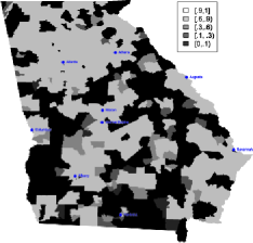
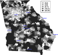
(a) Coverage	(b) Travel cost

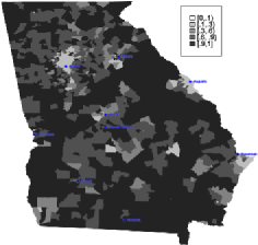
(c) Congestion

Figure 1: Estimated accessibility of children to primary care pediatricians, as measured by coverage rates, travel costs and congestion. Each measure of accessibility is derived using the proposed optimization approach. The maps show estimated accessibility in 2010 in census tracts in the state of Georgia.

With the exception of Atlanta, the state’s largest metro area, and Augusta, the location of the state’s medical school, there are only a handful of regions in the state with excellent accessibility across all three measures. Many of the rural and suburban areas that benefit from high coverage and low travel distances encounter high congestion, which highlights the importance of considering multiple dimensions of accessibility. High congestion can occur in rural areas if the region has a low supply of physicians relative to its population, or if the region is classified as a medically underserved area (MUA) and assumed to have the worst possible accessibility.

4.3 Evaluating policy interventions

Of the potential changes to the healthcare system that we consider, reductions in physicians’ participation in Medicaid programs have the most significant effect on patients’ accessibility. Table 2 and Figure 2 show that policies that reduce the number of physicians accepting Medicaid patients and policies that limit pediatricians’ Medicaid caseloads have similar impacts on Medicaid patients’ average accessibility. Both policies cause Medicaid patients’ average travel cost to increase by nearly 20%. Reducing $\mathrm{pam}$ has a slightly positive effect on Medicaid patients’ congestion, and reducing $\mathrm{MC}$ has a more substantial positive effect. One interpretation of these seemingly counterintuitive finding is that these policies reduce physicians’ total caseloads by restricting Medicaid patients’ access. Indeed, Medicaid patients’ coverage rates decrease by approximately 6 percentage points under these policies. This result also suggests that the burden of these policies may be unequally distributed among Medicaid patients, with some Medicaid patients experiencing little change in their accessibility and others finding that they now have no options for accessible medical care.

Table 2: This table shows the estimated effect of policies that reduce physicians’ participation in Medicaid programs. These polices and the interpretation of $\lambda$ are described in more detail in Section 3.2. For each policy, the first row shows the change in Georgia’s Medicaid patients’ state-wide, population-weighted average coverage rate, travel cost and congestion as one moves from the status quo to the maximum simulated reduction. The second row gives the percent change of these values

		Coverage rate	Travel cost	Congestion
Policy	$\bolds{\lambda}$	of Medicaid patients	of Medicaid patients	of Medicaid patients
$\mathrm{MC}$ scaling	$1\rightarrow 0.5$	$85.0\%\rightarrow 78.8\%$	$7.5\rightarrow 8.8$	$66.9\%\rightarrow 64.7\%$
		$(-7.2\%)$	(17.6%)	$(-3.2\%)$
$\mathrm{pam}$ scaling	$1\rightarrow 0.5$	$85.3\%\rightarrow 79.6\%$	$7.4\rightarrow 8.9$	$67.2\%\rightarrow 66.7\%$
		$(-6.7\%)$	(19.2%)	$(-0.6\%)$

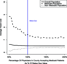
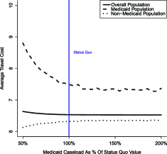
(a) Effect of changing pam	(b) Effect of changing MC

Figure 2: The impact of scaling policies on children’s state-wide, population-weighted average distance traveled to reach primary care pediatricians in Georgia. (a) shows the effects of policies that change the percentage of physicians accepting any Medicaid patients, while (b) shows the effects of policies that change the proportion of physicians’ caseloads that they are willing to devote to Medicaid patients.

Table 1 and Figures 6–8 in Supplementary Material D show that none of the initiatives designed to improve Medicaid patients’ accessibility deliver on their promise [Nobles, Serban and Swann (2014)]. The inability of these policies to create significant change in access to healthcare indicates that spatial accessibility may be limited by the current distribution of pediatricians. Among the 159 counties in Georgia, approximately $1/3$ have no pediatrician. Given this network of pediatricians, unless policies succeed in sending medical professionals to underserved areas, they are unlikely to accomplish substantial change. Examples of such policies include programs which forgive physicians’ graduate medical education loans in exchange for their practice in rural areas for a given period of time (http://gbpw.georgia.gov/loan-repayment-programs). Physicians may also be able to serve patients with limited accessibility through telemedicine initiatives [Marcin et al. (2004)]. Measuring the effects of these types of policies on accessibility is an interesting direction for future research.

4.4 Determining the effect of Medicaid participation on accessibility in Georgia

Figure 3 shows locations where one population has statistically significantly better accessibility than the other. As we would expect a priori, in many rural census tracts, other patients have significantly higher coverage and lower travel costs than Medicaid patients. Furthermore, there are no areas where Medicaid patients experience these advantages. We find that the direction of advantage is reversed for congestion, and there are many urban census tracts where Medicaid patients experience significantly lower congestion than other patients. Many physicians prefer privately insured patients to Medicaid patients and may be less likely to accept Medicaid patients if they can afford to only serve patients with private insurance. In regions where there is a high supply of physicians relative to the population, congestion is likely to be low and physicians may have greater incentive to accept all types of patients [Perloff, Kletke and Fossett (1995)]. Therefore, if Medicaid patients are able to be served by a physician, they may be more likely to experience lower congestion. Our results suggest that this theory holds true in Georgia.

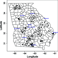
(a) Locations where other population	(b) Locations where Medicaid population
has significantly higher coverage	has significantly higher coverage
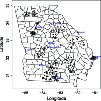
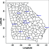
(c) Locations where other population	(d) Locations where Medicaid population
has significantly lower travel cost	has significantly lower travel cost
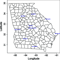
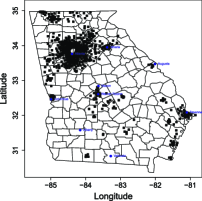
(e) Locations where other population	(f) Locations where Medicaid population
has significantly lower congestion	has significantly lower congestion

Figure 3: The points on these maps are the centroids of census tracts where there is a statistically significant difference in the accessibility of Medicaid patients and other patients.

Figure 9 in Supplementary Material D shows how these maps would change if physicians were to reduce their Medicaid caseload ($\mathrm{MC}$) by fifty percent [Nobles, Serban and Swann (2014)]. Under current conditions, there are 263 census tracts in Georgia where Medicaid patients experience statistically significantly higher travel costs than other patients. If policy changes prompt physicians to make these reductions in their Medicaid caseloads, this number would increase to 360. While this increase is considerable, there are also many communities whose access is unaffected by this shift in physicians’ attitudes. These findings further support our analysis in Section 4.3.

4.5 Factors associated with spatial accessibility in Georgia

Figure 10 in Supplementary Material D shows that accessibility is likely to be significantly higher than the population-weighted state-wide average in urban areas of Georgia, and significantly lower in rural regions of Georgia [Nobles, Serban and Swann (2014)]. This is especially true for coverage and travel cost. To determine if there are factors associated with these geographical disparities in accessibility, we apply the regression approach described in Section 3. Here, we run two sets of models: one where the dependent variable is the travel cost of the overall population and one where the dependent variable is the travel cost of the Medicaid population. The independent variables are chosen from the set of seven factors described in Section 3.3. Table 3 summarizes the results for the overall population based on the estimation of multiple models, each with four or more independent variables.

Table 3: The consistency, shape (constant vs. nonconstant), statistical significance and coefficient values observed across multiple models of the overall population’s travel cost in Georgia. These models each contain different combinations of the seven explanatory factors considered in the association analysis

Factor	Consistent	Significant	Shape	Range
Median household	Yes	Yes	Constant	[0.09, 0.37]
Income
Percent with higher education	No	Yes	Constant $\&$	$[-0.29,-0.26]$
			nonconstant	N/A
Unemployment rate	Yes	No	Constant	[0.026, 0.21]
Percent of nonwhite population	Yes	No	Constant	$[-0.18,0.63]$
Population density	Yes	Yes	Nonconstant	N/A
Distance to hospitals	No	Yes	Constant $\&$	[0.14, 0.16]
			nonconstant	N/A
Diversity ratio	Yes	Yes	Constant &	$[-0.23,-0.19]$
			nonconstant	N/A

While the results in Table 3 confirm that most factors commonly cited in the literature do indeed have a significant relationship with both populations’ spatial accessibility, there are two noteworthy exceptions: unemployment and race. We find more support for the emerging line of research which argues that the amount of racial diversity in a community is likely to be more strongly correlated with accessibility than race itself. Our diversity ratio measure is large when the amount of segregation in the immediate area is smaller than the amount of segregation in the greater surrounding region. In Georgia, this measure tends to be largest in small towns. When this measure has a constant effect on the overall population’s accessibility, the coefficient takes on a negative value, which implies that relatively diverse locations experience smaller travel costs.

Several variables have nonconstant effects on the overall population’s accessibility in some of the estimated models. Population density has a consistent nonconstant effect, while our measures of the education level, distance to hospitals and diversity ratio have constant effects in some models and nonconstant effects in others. Figure 4 shows a sample of these variables’ nonconstant association maps.

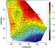
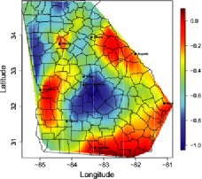
(a) Percent of population with higher education	(b) Population density measurement
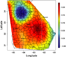
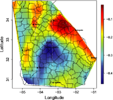
(c) Distance to hospitals measurement	(d) Diversity ratio measurement

Figure 4: Association map between the listed explanatory factor and the overall population’s travel cost to primary care pediatricians in Georgia.

While the inconsistency of these variables’ coefficients make interpretation more difficult, when these variables have a constant effect on travel cost, the direction of association is as expected: regions in Georgia with higher education levels, higher population density and smaller distances to hospitals travel shorter distances to primary care pediatricians. The median household income has a significant and positive constant association with accessibility, but our selection criteria are often superior in models where income is not included.

The consistency, significance and shape of the coefficients are identical in models of the overall population’s travel cost and in models of Medicaid patients’ travel cost. The range of the constant coefficients’ values are also very similar in the two sets of models. More detailed results are provided in Supplementary Material D [Nobles, Serban and Swann (2014)]. The consistency of these results is striking, and implies that the characteristics of vulnerable populations may not vary with insurance status.

In all of our models there is some variation in accessibility that remains unexplained. For the overall and Medicaid populations, the amount of spatial correlation in the models’ residuals ranges from $16.2\%$ to $42.7\%$, and from $34.3\%$ to $43.7\%$, respectively. There are several plausible explanations. First, researchers may have overlooked other factors that are the true drivers of accessibility. Alternatively, these factors may not identify locations where accessibility is superior to that of other regions with similar demographics, risk factors and resources. These anomalies are often the result of local community interventions. The fact that there is more unexplained variation in models of the Medicaid population’s accessibility suggests that local interventions which focus on improving Medicaid patients’ accessibility may be effective in changing the odds for these patients. While the concept of “positive deviance” has been explored in health outcomes [Pearce (2002); Walker et al. (2007)], there is little work on this with respect to accessibility and exploring this hypothesis would be an interesting direction for future research.

5 Conclusions

This paper introduces a comprehensive approach for making inferences about disparities in spatial accessibility. We develop and implement methodology for modeling accessibility that accounts for various constraints in the delivery system, including physicians’ characteristics and capacity. We simultaneously estimate multiple measures of accessibility including congestion, travel distance and coverage. By using an optimization-based approach, we can evaluate the implications of changes in the system, like those caused by policies which affect physician participation in Medicaid. Our measurement procedure is general, applicable to different types of care and scalable to varying geographic domains (e.g., state vs. national) and different network densities.

Our focus is on pediatric primary care accessibility. Using the models introduced in this paper, we find that there is a strong association between a community’s coverage rate and travel cost, but that there is more variability in congestion. The healthcare system is sensitive to reductions in physicians’ Medicaid caseload capacity, but resistant to many policies designed to improve accessibility. Population density, distance to hospitals, education and segregation levels are the factors most strongly associated with patients’ travel costs in Georgia.

One limitation of our optimization models is that the assignment solution is not unique. For example, we found five different ways to assign children to pediatricians in Georgia and satisfy our models’ constraints. Furthermore, our search was not exhaustive and there may be many more solutions. However, if two alternative solutions make small adjustments or trade-offs between immediate neighbors, the average accessibility in the community will not depend on the particular solution which is used. Indeed, we compared different solutions derived from our optimization model using statistical hypothesis testing, and we found that the difference between solutions is not statistically significant. We therefore conclude that our results will not be affected by the solution that we choose.

The precision of our results is also limited by the available data. Ideally, when implementing our models we would have data on each physician’s caseload and the extent of his or her participation in Medicaid programs. However, due to the sensitive nature of medical records and data, we only have aggregate estimates of this information. More detailed data on patient behavior, including their tolerance for congestion and the mobility of patients without access to cars, would also eliminate the need for several additional assumptions in our model. Finally, because we do not consider physicians located in neighboring states near the Georgia border, our results may suffer from edge effects. Therefore, our estimates of accessibility may be too low in census tracts close to the state line.

As mentioned throughout the paper, there are many avenues for future research related to accessibility measurement and inference. Interesting work could be done to model the effects of public transportation on patients’ accessibility, especially in urban areas. It is also important to consider the impact on accessibility of policies that would change the structure of the provider network. Furthermore, in this paper, we do not explore policies’ impact on health outcomes, like the number of emergency department visits. Addressing this question and further determining the relationship between accessibility to healthcare and health outcomes is an important extension of this work. Methods capable of evaluating the association between accessibility and a very large number of factors, including those not already highlighted by the literature, may also improve upon our regression models. Finally, studies should be done to consider accessibility in different states, for different types of healthcare and for many additional population groups. While this paper provides a basis for analyzing patients’ accessibility to healthcare, there is still much work to be done.

[id=suppA] Supplement to “Spatial accessibility of pediatric primary healthcare: Measurement and inference” [doi]10.1214/14-AOAS728SUPP .pdf aoas728_supp.pdf Supplementary Materials A, B, C and D contain four sections [Nobles, Serban and Swann (2014)]. In Supplementary Material A we describe methods that we utilized in our study but which are not essential components of our measurement and inference approach. In Supplementary Material B we give further details about the estimation of our space-varying coefficient model. In Supplementary Material C we provide additional details on the data sources we used to implement our models. In Supplementary Material D we present further results on children’s accessibility to primary care pediatricians in Georgia.

References

- Assuncao (2003) {barticle}[auto:parserefs-M02] \bauthor\bsnmAssuncao, \bfnmR. M.\binitsR. M. (\byear2003). \btitleSpace varying coefficient models for small area data. \bjournalEnvironmetrics \bvolume14 \bpages453–473. \bptokimsref\endbibitem
- Berman et al. (2002) {barticle}[auto:parserefs-M02] \bauthor\bsnmBerman, \bfnmS.\binitsS., \bauthor\bsnmDolins, \bfnmJ.\binitsJ. \betalet al. (\byear2002). \btitleFactors that influence the willingness of private primary care pediatricians to accept more Medicaid patients. \bjournalPediatrics \bvolume110 \bpages239–248. \bptokimsref\endbibitem
- Braveman and Gruskin (2003) {barticle}[auto:parserefs-M02] \bauthor\bsnmBraveman, \bfnmP.\binitsP. and \bauthor\bsnmGruskin, \bfnmS.\binitsS. (\byear2003). \btitleDefining equity in health. \bjournalJournal of Epidemiology and Community Health \bvolume57 \bpages254–258. \bptokimsref\endbibitem
- Buja, Hastie and Tibshirani (1989) {barticle}[mr] \bauthor\bsnmBuja, \bfnmAndreas\binitsA., \bauthor\bsnmHastie, \bfnmTrevor\binitsT. and \bauthor\bsnmTibshirani, \bfnmRobert\binitsR. (\byear1989). \btitleLinear smoothers and additive models. \bjournalAnn. Statist. \bvolume17 \bpages453–555. \biddoi=10.1214/aos/1176347115, issn=0090-5364, mr=0994249 \bptokimsref\endbibitem
- Diggle (1985) {barticle}[auto:parserefs-M02] \bauthor\bsnmDiggle, \bfnmP.\binitsP. (\byear1985). \btitleA Kernel method for smoothing point process data. \bjournalJ. R. Stat. Soc. Ser. C Appl. Stat. \bvolume34 \bpages138–147. \bptokimsref\endbibitem
- Drake and Rank (2009) {barticle}[auto:parserefs-M02] \bauthor\bsnmDrake, \bfnmB.\binitsB. and \bauthor\bsnmRank, \bfnmM. R.\binitsM. R. (\byear2009). \btitleThe racial divide among American children in poverty: Reassessing the importance of neighborhood. \bjournalChildren and Youth Services Review \bvolume31. \bptokimsref\endbibitem
- Fan and Zhang (2000) {barticle}[mr] \bauthor\bsnmFan, \bfnmJianqing\binitsJ. and \bauthor\bsnmZhang, \bfnmJin-Ting\binitsJ.-T. (\byear2000). \btitleTwo-step estimation of functional linear models with applications to longitudinal data. \bjournalJ. R. Stat. Soc. Ser. B Stat. Methodol. \bvolume62 \bpages303–322. \biddoi=10.1111/1467-9868.00233, issn=1369-7412, mr=1749541 \bptokimsref\endbibitem
- Fiscella and Williams (2004) {barticle}[auto:parserefs-M02] \bauthor\bsnmFiscella, \bfnmK.\binitsK. and \bauthor\bsnmWilliams, \bfnmD.\binitsD. (\byear2004). \btitleHealth disparities based on socioeconomic inequities: Implications for urban health care. \bjournalAcademic Medicine \bvolume79 \bpages1139–1147. \bptokimsref\endbibitem
- Fleurbaey and Schokkaert (2009) {barticle}[auto:parserefs-M02] \bauthor\bsnmFleurbaey, \bfnmM.\binitsM. and \bauthor\bsnmSchokkaert, \bfnmE.\binitsE. (\byear2009). \btitleUnfair inequalities in health and health care. \bjournalJournal of Health Economics \bvolume28 \bpages73–90. \bptokimsref\endbibitem
- Gelfand et al. (2003) {barticle}[mr] \bauthor\bsnmGelfand, \bfnmAlan E.\binitsA. E., \bauthor\bsnmKim, \bfnmHyon-Jung\binitsH.-J., \bauthor\bsnmSirmans, \bfnmC. F.\binitsC. F. and \bauthor\bsnmBanerjee, \bfnmSudipto\binitsS. (\byear2003). \btitleSpatial modeling with spatially varying coefficient processes. \bjournalJ. Amer. Statist. Assoc. \bvolume98 \bpages387–396. \biddoi=10.1198/016214503000170, issn=0162-1459, mr=1995715 \bptokimsref\endbibitem
- Guagliardo (2004) {barticle}[auto:parserefs-M02] \bauthor\bsnmGuagliardo, \bfnmM. F.\binitsM. F. (\byear2004). \btitleSpatial accessibility of primary care: Concepts, methods and challenges. \bjournalInternational Journal of Health Geographics \bvolume3 \bpages1–13. \bptokimsref\endbibitem
- Guagliardo et al. (2004) {barticle}[auto] \bauthor\bsnmGuagliardo, \bfnmM. F.\binitsM. F., \bauthor\bsnmRonzio, \bfnmC. R.\binitsC. R., \bauthor\bsnmCheung, \bfnmI.\binitsI., \bauthor\bsnmChacko, \bfnmE.\binitsE. and \bauthor\bsnmJoseph, \bfnmJ. G.\binitsJ. G., (\byear2004). \btitlePhysician accessibility: An urban case study of pediatric providers. \bjournalHealth Place \bvolume10 \bpages273–283. \bptokimsref\endbibitem
- Hambidge et al. (2007) {barticle}[auto:parserefs-M02] \bauthor\bsnmHambidge, \bfnmS.\binitsS., \bauthor\bsnmEmsermann, \bfnmC.\binitsC. \betalet al. (\byear2007). \btitleDisparities in pediatric preventive care in the United States. \bjournalArchives of Pediatric and Adolescent Medicine \bvolume161 \bpages30–36. \bptokimsref\endbibitem
- Hastie and Tibshirani (1990) {bbook}[mr] \bauthor\bsnmHastie, \bfnmT. J.\binitsT. J. and \bauthor\bsnmTibshirani, \bfnmR. J.\binitsR. J. (\byear1990). \btitleGeneralized Additive Models. \bseriesMonographs on Statistics and Applied Probability \bvolume43. \bpublisherChapman & Hall, \blocationLondon. \bidmr=1082147 \bptokimsref\endbibitem
- Hastie and Tibshirani (1993) {barticle}[mr] \bauthor\bsnmHastie, \bfnmTrevor\binitsT. and \bauthor\bsnmTibshirani, \bfnmRobert\binitsR. (\byear1993). \btitleVarying-coefficient models. \bjournalJ. R. Stat. Soc. Ser. B Stat. Methodol. \bvolume55 \bpages757–796. \bidissn=0035-9246, mr=1229881 \bptnotecheck related \bptokimsref\endbibitem
- Hoover et al. (1998) {barticle}[mr] \bauthor\bsnmHoover, \bfnmDonald R.\binitsD. R., \bauthor\bsnmRice, \bfnmJohn A.\binitsJ. A., \bauthor\bsnmWu, \bfnmColin O.\binitsC. O. and \bauthor\bsnmYang, \bfnmLi-Ping\binitsL.-P. (\byear1998). \btitleNonparametric smoothing estimates of time-varying coefficient models with longitudinal data. \bjournalBiometrika \bvolume85 \bpages809–822. \biddoi=10.1093/biomet/85.4.809, issn=0006-3444, mr=1666699 \bptokimsref\endbibitem
- Jiang (2010) {bmisc}[auto] \bauthor\bsnmJiang, \bfnmH.\binitsH. (\byear2010). \bhowpublishedStatistical computation and inference for functional data analysis. Ph.D. thesis, Georgia Institute of Technology, Atlanta, GA. \bptokimsref\endbibitem
- Joseph and Phillips (1984) {bbook}[auto:parserefs-M02] \bauthor\bsnmJoseph, \bfnmA.\binitsA. and \bauthor\bsnmPhillips, \bfnmD.\binitsD. (\byear1984). \btitleAccessibility and Utilization: Geographical Perspectives on Health Care Delivery. \bpublisherHarper and Row, \blocationNew York. \bptokimsref\endbibitem
- Khan (1992) {barticle}[auto:parserefs-M02] \bauthor\bsnmKhan, \bfnmA.\binitsA. (\byear1992). \btitleAn integrated approach to measuring potential spatial access to healthcare services. \bjournalSocio-Economic Planning Sciences \bvolume26 \bpages275–287. \bptokimsref\endbibitem
- Kids Count National Indicators (2010) {bmisc}[auto] \borganizationKids Count National Indicators (\byear2010). \bhowpublishedData Center, Baltimore MD. \bptokimsref\endbibitem
- Krivobokova, Kneib and Claeskens (2010) {barticle}[mr] \bauthor\bsnmKrivobokova, \bfnmTatyana\binitsT., \bauthor\bsnmKneib, \bfnmThomas\binitsT. and \bauthor\bsnmClaeskens, \bfnmGerda\binitsG. (\byear2010). \btitleSimultaneous confidence bands for penalized spline estimators. \bjournalJ. Amer. Statist. Assoc. \bvolume105 \bpages852–863. \biddoi=10.1198/jasa.2010.tm09165, issn=0162-1459, mr=2724866 \bptokimsref\endbibitem
- Li and Ruppert (2008) {barticle}[mr] \bauthor\bsnmLi, \bfnmYingxing\binitsY. and \bauthor\bsnmRuppert, \bfnmDavid\binitsD. (\byear2008). \btitleOn the asymptotics of penalized splines. \bjournalBiometrika \bvolume95 \bpages415–436. \biddoi=10.1093/biomet/asn010, issn=0006-3444, mr=2521591 \bptokimsref\endbibitem
- Luo and Qi (2009) {barticle}[pbm] \bauthor\bsnmLuo, \bfnmWei\binitsW. and \bauthor\bsnmQi, \bfnmYi\binitsY. (\byear2009). \btitleAn enhanced two-step floating catchment area (E2SFCA) method for measuring spatial accessibility to primary care physicians. \bjournalHealth Place \bvolume15 \bpages1100–1107. \biddoi=10.1016/j.healthplace.2009.06.002, issn=1353-8292, pii=S1353-8292(09)00057-4, pmid=19576837 \bptokimsref\endbibitem
- Marcin et al. (2004) {barticle}[auto:parserefs-M02] \bauthor\bsnmMarcin, \bfnmJ.\binitsJ., \bauthor\bsnmEllis, \bfnmJ.\binitsJ. \betalet al. (\byear2004). \btitleUsing telemedicine to provide pediatric subspecialty care to children with special health care needs in an underserved rural community. \bjournalPediatrics \bvolume13 \bpages1–6. \bptokimsref\endbibitem
- Marmot et al. (2008) {barticle}[auto:parserefs-M02] \bauthor\bsnmMarmot, \bfnmM.\binitsM., \bauthor\bsnmFriel, \bfnmS.\binitsS. \betalet al. (\byear2008). \btitleClosing the gap in a generation: Health equity through action on the social determinants of health. \bjournalLancet \bvolume372 \bpages1661–1669. \bptokimsref\endbibitem
- Marsh and Schilling (1994) {barticle}[auto:parserefs-M02] \bauthor\bsnmMarsh, \bfnmM. T.\binitsM. T. and \bauthor\bsnmSchilling, \bfnmD. A.\binitsD. A. (\byear1994). \btitleEquity measurement in facility location analysis: A review and framework. \bjournalEuropean J. Oper. Res. \bvolume74 \bpages1–17. \bptokimsref\endbibitem
- McGrail and Humphreys (2009) {barticle}[auto:parserefs-M02] \bauthor\bsnmMcGrail, \bfnmM. R.\binitsM. R. and \bauthor\bsnmHumphreys, \bfnmJ. S.\binitsJ. S. (\byear2009). \btitleThe index of rural access: An innovative integrated approach for measuring primary care access. \bjournalBMC Health Services Research \bvolume9. \bnoteDOI:\doiurl10.1186/1472-6963-9-124. \bptokimsref\endbibitem
- Nobles, Serban and Swann (2014) {bmisc}[author] \bauthor\bsnmNobles, \bfnmM.\binitsM., \bauthor\bsnmSerban, \bfnmN.\binitsN. and \bauthor\bsnmSwann, \bfnmJ.\binitsJ. (\byear2014). \bhowpublishedSupplement to “Spatial accessibility of pediatric primary healthcare: Measurement and inference.” DOI:\doiurl10.1214/14-AOAS728SUPP. \bptokimsref \endbibitem
- Odoki, Kerali and Santorini (2001) {barticle}[auto:parserefs-M02] \bauthor\bsnmOdoki, \bfnmJ.\binitsJ., \bauthor\bsnmKerali, \bfnmH.\binitsH. and \bauthor\bsnmSantorini, \bfnmF.\binitsF. (\byear2001). \btitleAn integrated model for quantifying accessibility-benefits in developing countries. \bjournalTransportation Research Part A: Policy and Practice \bvolume35 \bpages601–623. \bptokimsref\endbibitem
- Parzen (1962) {barticle}[mr] \bauthor\bsnmParzen, \bfnmEmanuel\binitsE. (\byear1962). \btitleOn estimation of a probability density function and mode. \bjournalAnn. Math. Statist. \bvolume33 \bpages1065–1076. \bidissn=0003-4851, mr=0143282 \bptokimsref\endbibitem
- Pearce (2002) {barticle}[auto:parserefs-M02] \bauthor\bsnmPearce, \bfnmL. D.\binitsL. D. (\byear2002). \btitleIntegrating survey and ethnographic models for systematic anomalous case analysis. \bjournalSociological Methodology \bvolume32 \bpages103–132. \bptokimsref\endbibitem
- Penchansky and Thomas (1981) {barticle}[auto:parserefs-M02] \bauthor\bsnmPenchansky, \bfnmR.\binitsR. and \bauthor\bsnmThomas, \bfnmJ. W.\binitsJ. W. (\byear1981). \btitleThe concept of access. \bjournalMed. Care \bvolume19 \bpages127–140. \bptokimsref\endbibitem
- Perloff, Kletke and Fossett (1995) {barticle}[auto:parserefs-M02] \bauthor\bsnmPerloff, \bfnmJ.\binitsJ., \bauthor\bsnmKletke, \bfnmP.\binitsP. and \bauthor\bsnmFossett, \bfnmJ.\binitsJ. (\byear1995). \btitleWhich physicians limit their Medicaid participation, and why. \bjournalHealth Services Research \bvolume30 \bpages7–25. \bptokimsref\endbibitem
- Reardon et al. (2008) {barticle}[pbm] \bauthor\bsnmReardon, \bfnmSean F.\binitsS. F., \bauthor\bsnmMatthews, \bfnmStephen A.\binitsS. A., \bauthor\bsnmO’Sullivan, \bfnmDavid\binitsD., \bauthor\bsnmLee, \bfnmBarrett A.\binitsB. A., \bauthor\bsnmFirebaugh, \bfnmGlenn\binitsG., \bauthor\bsnmFarrell, \bfnmChad R.\binitsC. R. and \bauthor\bsnmBischoff, \bfnmKendra\binitsK. (\byear2008). \btitleThe geographic scale of metropolitan racial segregation. \bjournalDemography \bvolume45 \bpages489–514. \bidissn=0070-3370, pmcid=2831394, pmid=18939658 \bptokimsref\endbibitem
- Ruppert, Wand and Carroll (2003) {bbook}[mr] \bauthor\bsnmRuppert, \bfnmDavid\binitsD., \bauthor\bsnmWand, \bfnmM. P.\binitsM. P. and \bauthor\bsnmCarroll, \bfnmR. J.\binitsR. J. (\byear2003). \btitleSemiparametric Regression. \bseriesCambridge Series in Statistical and Probabilistic Mathematics \bvolume12. \bpublisherCambridge Univ. Press, \blocationCambridge. \biddoi=10.1017/CBO9780511755453, mr=1998720 \bptokimsref\endbibitem
- Serban (2011) {barticle}[mr] \bauthor\bsnmSerban, \bfnmNicoleta\binitsN. (\byear2011). \btitleA space–time varying coefficient model: The equity of service accessibility. \bjournalAnn. Appl. Stat. \bvolume5 \bpages2024–2051. \biddoi=10.1214/11-AOAS473, issn=1932-6157, mr=2884930 \bptokimsref\endbibitem
- Talen and Anselin (1998) {barticle}[auto:parserefs-M02] \bauthor\bsnmTalen, \bfnmE.\binitsE. and \bauthor\bsnmAnselin, \bfnmL.\binitsL. (\byear1998). \btitleAssessing spatial equity: An evaluation of measures of accessibility to public playgrounds. \bjournalEnvironment and Planning B: Planning and Design \bvolume30 \bpages595. \bptokimsref\endbibitem
- Tibshirani and Knight (1999) {barticle}[mr] \bauthor\bsnmTibshirani, \bfnmRobert\binitsR. and \bauthor\bsnmKnight, \bfnmKeith\binitsK. (\byear1999). \btitleThe covariance inflation criterion for adaptive model selection. \bjournalJ. R. Stat. Soc. Ser. B Stat. Methodol. \bvolume61 \bpages529–546. \biddoi=10.1111/1467-9868.00191, issn=1369-7412, mr=1707859 \bptokimsref\endbibitem
- Walker et al. (2007) {barticle}[pbm] \bauthor\bsnmWalker, \bfnmLorraine O.\binitsL. O., \bauthor\bsnmSterling, \bfnmBobbie Sue\binitsB. S., \bauthor\bsnmHoke, \bfnmMary M.\binitsM. M. and \bauthor\bsnmDearden, \bfnmKirk A.\binitsK. A. (\byear2007). \btitleApplying the concept of positive deviance to public health data: A tool for reducing health disparities. \bjournalPublic Health Nurs. \bvolume24 \bpages571–576. \biddoi=10.1111/j.1525-1446.2007.00670.x, issn=0737-1209, pii=PHN670, pmid=17973735 \bptokimsref\endbibitem
- Waller et al. (2007) {barticle}[mr] \bauthor\bsnmWaller, \bfnmLance A.\binitsL. A., \bauthor\bsnmZhu, \bfnmLi\binitsL., \bauthor\bsnmGotway, \bfnmCarol A.\binitsC. A., \bauthor\bsnmGorman, \bfnmDennis M.\binitsD. M. and \bauthor\bsnmGruenewald, \bfnmPaul J.\binitsP. J. (\byear2007). \btitleQuantifying geographic variations in associations between alcohol distribution and violence: A comparison of geographically weighted regression and spatially varying coefficient models. \bjournalStoch. Environ. Res. Risk Assess. \bvolume21 \bpages573–588. \biddoi=10.1007/s00477-007-0139-9, issn=1436-3240, mr=2380676 \bptokimsref\endbibitem
- Wang and Luo (2005) {barticle}[pbm] \bauthor\bsnmWang, \bfnmFahui\binitsF. and \bauthor\bsnmLuo, \bfnmWei\binitsW. (\byear2005). \btitleAssessing spatial and nonspatial factors for healthcare access: Towards an integrated approach to defining health professional shortage areas. \bjournalHealth Place \bvolume11 \bpages131–146. \biddoi=10.1016/j.healthplace.2004.02.003, issn=1353-8292, pii=S1353829204000085, pmid=15629681 \bptokimsref\endbibitem
- Williams and Mohammed (2009) {barticle}[auto:parserefs-M02] \bauthor\bsnmWilliams, \bfnmD. R.\binitsD. R. and \bauthor\bsnmMohammed, \bfnmS. A.\binitsS. A. (\byear2009). \btitleDiscrimination and racial disparities in health: Evidence and needed research. \bjournalJournal of Behavioral Medicine \bvolume32 \bpages20–47. \bptokimsref\endbibitem
- Wu and Liang (2004) {barticle}[auto:parserefs-M02] \bauthor\bsnmWu, \bfnmH.\binitsH. and \bauthor\bsnmLiang, \bfnmH.\binitsH. (\byear2004). \btitleBackfitting random varying-coefficient models with timedependent smoothing covariates. \bjournalScand. J. Stat. \bvolume31 \bpages320–330. \bptokimsref\endbibitem