Unbinding transition in semi-infinite two-dimensional localized systems

Abstract

We consider a two-dimensional strongly localized system defined in a half-space and whose transfer integral in the edge can be different than in the bulk. We predict an unbinding transition, as the edge transfer integral is varied, from a phase where conduction paths are distributed across the bulk to a bound phase where propagation is mainly along the edge. At criticality the logarithm of the conductance follows the $F_{1}$ Tracy-Widom distribution. We verify numerically these predictions for both the Anderson and the Nguyen, Spivak and Shklovskii models. We also check that for a half-space, i.e., when the edge transfer integral is equal to the bulk transfer integral, the distribution of the conductance is the $F_{4}$ Tracy-Widom distribution. These findings are strong indications that random signs directed polymer models and their quantum extensions belong to the Kardar-Parisi-Zhang universality class. We have analyzed finite-size corrections at criticality and for a half-plane.

The probability distribution function of the conductance $g$ of quantum random hopping models, such as the Anderson model, has been much studied. In one dimension, it has been shown that all the cumulants of $\ln g$ scale linearly with system size Ro92 . Thus, the distribution function of $\ln g$ approaches a Gaussian form for asymptotically long systems and is fully characterized by two parameters, the mean $\langle\ln g\rangle$ and the variance $\sigma^{2}=\langle\ln^{2}g\rangle-\langle\ln g\rangle^{2}$. Both parameters are related to each other, supporting the extension of the single parameter scaling hypothesis AA79 to the distribution function of the conductance shapiro .

In two-dimensional (2D) systems, calculations of the conductance distribution function are possible in the metallic regime, thanks to the non-linear sigma model 2D , but not until now in the strongly localized regime. However, two of us have argued, and demonstrated numerically, that in that regime $L\gg\xi$, $\xi$ being the localization length, the conductance takes the form SoOr07 ; PS05

$$\ln g=-\frac{2L}{\xi}+\alpha\left(\frac{L}{\xi}\right)^{1/3}\chi$$ (1)

where $\alpha$ is a constant and $\chi$ a random variable with a Tracy-Widom (TW) cumulative distribution function (CDF). The TW distributions are CDF for the largest eigenvalues of large Gaussian random matrices TW . It was found that the random variable $\chi$ depends on the geometry of the model. For narrow leads, the TW distribution associated to the Gaussian unitary ensemble $\chi=\chi_{2}$ is the CDF $F_{2}(x)$, i.e., ${\rm Prob}(\chi_{2}<x)=F_{2}(x)=F(x)^{2}$, where $F(x)$ is defined as $F(x)=\exp\{-\frac{1}{2}\int_{x}^{+\infty}(s-x)u(s)^{2}ds\}$ and $u(x)$ is the solution of the Painlevé II equation $u^{\prime\prime}(x)=2u(x)^{3}+xu(x)$, with $u(x)\rightarrow-{\rm Ai}(x)$ as $x\rightarrow+\infty$, ${\rm Ai}(x)$ being the Airy function.

The chain of arguments leading to (1) goes as follows. It was argued by Nguyen et al. (NSS) NS85 that quantum interference effects in the localized regime are faithfully described by retaining only the shortest or forward-scattering paths. Medina and Kardar MK92 studied in detail the NSS model, focusing on its formulation as a model of directed polymers (DP) with non-positive Boltzmann weights. They found that the variance of the tunneling probability increases with distance as $L^{2/3}$ for 2D systems. This suggests that in 2D the DP with non-positive Boltzmann weights should be in the same universality class as the standard (i.e. positive weight) DP problem, well known to exhibit a wandering exponent of $2/3$. A qualitative replica argument led to the same conclusion MK92 .

In the mean-time, much progress happened in the study of growth models in the Kardar-Parisi-Zhang (KPZ) universality class KPZ . The standard DP problem belongs to this class (the KPZ height $h$ maps onto $\ln Z$ where $Z$ is the DP partition sum). Remarkably, it was found that the TW distribution arises at large time scales (i.e. long polymer length) in discrete models in the KPZ class. For example, the height in the polynuclear growth model png , the optimal energy in DP models Johansson , and the length of the longest increasing subsequence in a random permutation BD99 all follow TW distributions.

This body of facts thus led to the conjecture (1) with the $1/3$ exponent of the KPZ class, and to its numerical verification. More recently the KPZ equation and the DP problem have been solved directly in the continuum, using integrability by the Bethe Ansatz of an associated quantum boson model we ; dotsenko ; spohnKPZEdge ; corwinDP . Various boundary conditions where treated, suggesting new tests for the conjecture (1) with various lead geometries. In particular the continuum DP problem in a half-space was found we-halfspace to lead to the $F_{4}$ TW distribution, associated to the Gaussian simplectic ensemble, in agreement with earlier results for discrete models sasamotohalfspace ; BaikSymPermutations . This distribution verifies $F_{4}(x)=F(x)(E(x)^{-1}+E(x))/2$ where $E(x)=\exp\{\frac{1}{2}\int_{x}^{+\infty}u(s)ds\}$, $F(x)$ and $u(x)$ are the functions defined above. It was thus conjectured we-halfspace that in a half-space the conductance near the edge should be of the form (1) with $\chi=\chi_{4}$ of CDF given by $F_{4}$.

The aim of this paper is to study the logarithm of the conductance $\ln g$ in 2D systems in the strongly localized regime in order to (i) verify numerically the conjecture that the CDF of for a half-plane is the $F_{4}(x)$ function, and (ii) predict and analyze the transition from 2D to 1D as the hopping amplitude $t$ at the edge is increased, favoring propagation along the edge. Exactly at criticality we observe that the CDF of $\ln g$ is the TW distribution $F_{1}(x)=F(x)E(x)$ of the Gaussian orthogonal ensemble. This transition is a generalization of the unbinding transition studied for positive weight DP Kardar ; BaikSymPermutations . Remarkably, the full crossover distribution obtained there fits our data for the whole parameter range, providing a very delicate test that the random sign DP belongs to the KPZ universality class. This is all the more precious since at present no integrable system has been found to solve the NSS model.

We focus on the Anderson model on a square sample of finite size $L\times L$ described by the Hamiltonian

$$H=\sum_{i}\epsilon_{i}a_{i}^{\dagger}a_{i}+\sum_{\langle i,j\rangle}t_{i,j}a_{j}^{\dagger}a_{i}+{\rm h.c.}\;,$$ (2)

where the operator $a_{i}^{\dagger}$ ($a_{i}$) creates (destroys) an electron at site $i$ of an square lattice and $\epsilon_{i}$ is the energy of this site chosen at random $\epsilon_{i}\in[-W/2,W/2]$, with $W$ the strength of the disorder. The double sum runs over nearest neighbors. The hopping matrix element $t_{i,j}$ is taken equal to $1$ everywhere, except between the sites along one edge where is equal $t>1$ (see figure 1). The value in the bulk sets the energy scale, while the lattice constant sets the length scale. The unit of conductance is $2e^{2}/h$.

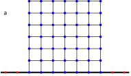
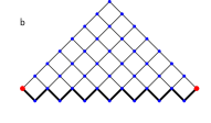
Figure 1: Scheme of the geometrical arrangements of the a) Anderson model, and the b) NSS model. Blue dots are site with random disorder energies and red dots sites on the leads, without disorder. Thin lines correspond to the bulk hopping strength equal 1, while thick lines along the edge to $t$.

For the Anderson model we have calculated the conductance through Landauer’s formula in terms of the transmission between perfect leads, arranged as schematically shown in Fig. 1a. This is obtained from the Green function, which can be calculated propagating layer by layer M85 . It is convenient to propagate along the direction perpendicular to the leads, starting from the opposite edge, so that each calculation of the bulk Green function can be used for any value of $t$.

The Green function between two sites $a$ and $b$ can be written in terms of the locator expansion

$$\langle a|G|b\rangle=\sum_{\Gamma}\prod_{i\in\Gamma}\frac{1}{E-\epsilon_{i}}\;,$$ (3)

where the sum runs over all possible paths connecting the two sites $a$ and $b$. The NSS model assumes that, in the strongly localized regime, (3) is dominated by the forward-scattering paths and only takes into account the contributions of such paths to the transmission amplitude between opposite corners of a square lattice. As we want to study a half-space, we consider a triangular sample as represented in Fig. 1b. In order to mimic the Anderson model, we choose the site disorder energy at random in the interval $\epsilon_{i}\in[-W/2,W/2]$, but if $|E-\epsilon_{i}|<1$, we set $1/|E-\epsilon_{i}|=1$, partially incorporating multiple scattering effects. We note that at least for the planar symmetry this choice of disorder does no change the universality of the problem epl .

The calculation of the quantum amplitude in the NSS model is formally similar to the calculation of the partition function of DP in a random potential

$$Z=\sum_{\Gamma}\exp\left\{-\beta\sum_{i\in\Gamma}h_{i}\right\}\;,$$ (4)

where $\beta=1/kT$, $h_{i}$ is a random site energy and $\Gamma$ runs over all possible configurations of the DP. Equations (3) and (4) are equivalent provided that we can identify $-\beta h_{i}$ with $\ln(E-\epsilon_{i})$. While in DP the disorder energies $h_{i}$ are real, in the quantum case $E-\epsilon_{i}$ does not have to be positive, implying a more general problem.

It is interesting to study first the conductance distribution of the NSS and Anderson models in a half-space and check whether the conjecture of Ref. we-halfspace , based on the exact result for the continuum DP, that the CDF of $\chi$ is the TW function $F_{4}$ is verified by our two models. In Fig. 2 we plot histograms of $\ln g$ for the NSS model as a function of $z=(\ln g-A)/B$, where $A$ and $B$ are chosen so that $z$ has the same mean and variance as $F_{4}$. The lateral dimensions are $L=2500$ (blue dots), 5000 (red dots) and 10000 (black dots), and the number of realizations is $4\times 10^{6}$. The solid line corresponds to the TW function $F_{4}^{\prime}$. We see a perfect agreement between our numerical results and the TW distribution for more than four orders of magnitude. A similar agreement is found for the Anderson model (not shown), taking into account that it corresponds to smaller system sizes.

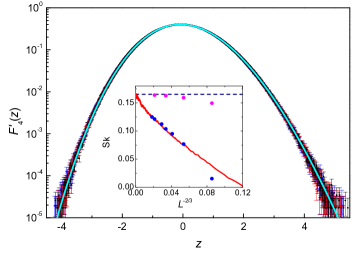
Figure 2: Histogram of $\ln g$ versus the scaled variable $z$ for three sizes and a disorder $W=10$ of the NSS model. The continuous line corresponds to $F_{4}^{\prime}(z)$. Inset: skewness vs. $L^{-2/3}$ for the NSS model (red curve) for the Anderson model with $W=10$ (blue dots) and 20 (magenta dots); the dashed line is Sk₄.

The inset of Fig. 2 we plot the skewness of $\ln g$ versus $L^{-2/3}$, which according to the discussion below is expected to be the leading order correction. The red line corresponds to the NSS model, while the dots to the Anderson model ($W=10$ blue, 20 magenta). The dashed line is Sk${}_{4}=0.165509...$ The skewness of the numerical results for both models tends to the predicted value.

We now argue theoretically that the NSS and the Anderson models exhibit a phase transition between (i) a 2D phase where conduction paths wander unboundedly in the half-space and the fluctuations of $\ln g$ at large $L$ are described by (1) with $\chi=\chi_{4}$, and (ii) a quasi-1D localized phase where the conduction paths have 1D character at large scale, and $\ln g$ has a log-normal distribution with fluctuations scaling as $L^{1/2}$, i.e. (1) still holds but with a size dependent variable $\chi\to\chi_{L}$, scaling now as $\chi_{L}\sim L^{-1/6}$. Exactly at the transition $t=t_{\rm c}$, the fluctuations of $\ln g$ at large $L$ are described by (1) with now $\chi=\chi_{1}$ distributed according to $F_{1}$. Hence the 1/3 KPZ exponent holds up to and at the transition. This transition can be described as an unbinding transition of conduction paths. In the standard DP the unbinding transition was predicted in Kardar and worked out in detail in the framework of symmetrized random permutations in BaikSymPermutations . Before using these results below, let us first give the physical picture and the scaling arguments.

In the unbound phase, $t>t_{\rm c}$, the paths wander in the 2D space, but come back from time to time to the boundary (they still feel the boundary hence the change from $F_{1}$ to $F_{4}$). Their typical transverse wandering is $L^{2/3}$. Ins the bound phase, the paths return to the wall, with a typical length $\xi_{u}$ which diverges at the transition as $\xi_{u}\sim(t-t_{\rm c})^{-3}$. Near the transition there are thus $L/\xi_{u}$ independent pieces of paths, each fluctuating as $\xi_{u}^{1/3}$ hence the variance should behave as $\overline{(\ln g)^{2}}^{c}=\xi_{u}^{2/3}(L/\xi_{u})=L/\xi_{u}^{1/3}\sim(t-t_{\rm c})L$. Far from the transition this picture predicts that the skewness should decay as Sk$\sim(L/\xi_{u})^{-1/2}$, since in the 1D phase the central limit theorem holds for $\ln g$ and all cumulants scale as $L$ i.e. $\overline{(\ln g)^{n}}^{c}\sim L$.

Let us now consider the critical scaling around the transition point BaikSymPermutations . Our prediction is that $\ln g$ always behaves as in (1) with the random variable $\chi$ having a CDF Prob$(\chi<x)={\cal F}(x,w=-c\tilde{w})$ that depends on the scaling variable $\tilde{w}=(t-t_{\rm c})L^{1/3}$, $c>0$ being an (unknown) proportionality constant. The universal crossover function ${\cal F}(x,w)$ (corresponding to $F^{\boxslash}(x,w/2)$ in Ref. BaikSymPermutations, ) satisfies

$${\cal F}(x,w)=\frac{1}{2}F(x)\big{(}(f(x,w)-g(x,w))E(x)^{-1}$$ (5)

$$+(f(x,w)+g(x,w))E(x)\big{)}$$

where the functions $f(x,w)$ and $g(x,w)$ are the ones of Baik2 and verify:

$$\partial_{w}f(x,w) = u(x)^{2}f(x,w)-(wu(x)+u^{\prime}(x))g(x,w)$$

$$\partial_{w}g(x,w) = -(wu(x)-u^{\prime}(x))f(x,w)+$$ (6)

$$(w^{2}-x-u^{2}(x))g(x,w)$$

and are subjected to the initial condition at criticality $f(x,0)=-g(x,0)=E(x)^{2}$. Then, the CDF at criticality is ${\cal F}(x,0)=F_{1}(x)$. In the limit $w\to+\infty$, one has $f\to 1$ and $g\to 0$, hence ${\cal F}(x,\infty)=F_{4}$. In the opposite limit, $w\to-\infty$ Baik2 ${\cal F}(w^{2}+y\sqrt{|w|},w)\to{\rm erf}(y)$ and one recovers Gaussian fluctuations for $\ln g$.

To study the transition and to characterize the two phases, we analyze the skewness of the distribution of $\ln g$ for the NSS model as we vary $t$. The skewness should tend to 0 in the localized phase, to Sk${}_{1}=0.293464...$ at the transition and to Sk₄ in the unbound phase. In Fig. 3 we plot the skewness as a function of size on a logarithmic scale for several values of the edge strength $t$. The upper horizontal line corresponds to the expected value of the skewness at the critical point, Sk₁, and the lower horizontal line to the limiting value in the bulk phase, Sk₄. The black curve represents the skewness at the critical value $t_{\rm c}\approx 1.613(1)$ and tends to the upper horizontal line, Sk₁. Solid curves are for $t>t_{\rm c}$ and after reaching a maximum start decreasing, eventually tending to zero. Dashed lines correspond to $t<t_{\rm c}$ and tend to Sk₄, middle horizontal line in Fig. 3.

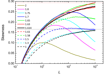
Figure 3: Skewness versus $L$ on a logarithmic scale for the values of $t$ shown in the figure. The red dashed line corresponds to Sk₁ and the dashed black horizontal line to Sk₄.

It is possible to scale the raw data for the skewness at large values of $L$ into a universal curve using as scaling variable ${\tilde{w}}=(t-t_{\rm c})L^{1/3}$. Looking at the behavior of the skewness for the critical value $t_{\rm c}$ in Fig. 3, it is clear that finite size effects are important. To take them into account we assume Sk$(t,L)\approx\mbox{Sk}(\tilde{w})f(L)$, where $f(L)$ incorporates finite size effects in a simple way $f(L)=\mbox{Sk}(t_{\rm c},L)/\mbox{Sk}_{1}$. In Fig. 4 we plot this renormalized values Sk$(\tilde{w})$ for several values of $t$. All curves are plotted for the range $200<L<10^{4}$. The black dot represents the transition point and so is equal Sk₁ and is placed at the vertical axis, $t=t_{\rm c}$. The dashed line is the theoretical prediction for the scaling function, i.e., the solution of Eqs. (6), using a value $c=0.9$ for the multiplicative constant. It presents a maximum in the localized phase well reproduced by our simulations. The blue dotted line on the right represents the limiting behavior in the bound phase, $b\tilde{w}^{-3/2}$, with the fitting parameter $b=0.55$. The overlap and the agreement with theoretical expectations is quite good, specially noting that the only free parameter to overlap all the curves is $t_{\rm c}$.

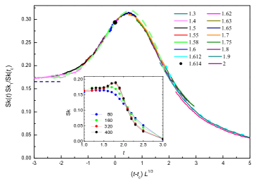
Figure 4: Skewness scaled as a function of ${\tilde{w}}=(t-t_{\rm c})L^{1/3}$ for several values of $t$. The black dot corresponds to Sk₁ at the transition and the horizontal dashed line to Sk₄. The dashed curve is the theoretical prediction for the scaling function and the dotted curve the predicted asymptotic behavior at large $\tilde{w}$. Inset: skewness as a function of $t$ for the Anderson model.

The results for the Anderson model confirm all predictions, although the maximum size that can be calculated, $L=400$, is still relatively far from the asymptotic behavior. In the inset of Fig. 4, we plot the skewness as a function of $t$ for several system sizes of the Anderson model and a disorder $W=20$. A peak around $t\approx 1.8$ develops with size, but its maximum is still far from Sk₁. This results are fully consistent with NSS for similar sizes.

It is interesting to compare the finite size corrections in our models with those for discrete growth models and experiments in the KPZ class. Consider $K_{n}$ the cumulant of $\ln g$ (here) and of the interface height $h$ (there, time being denoted as $L$) and the scaled cumulants $k_{n}=K_{n}/L^{n/3}$ which converge to constants. The finite size corrections of the $k_{n}$ where found (there in the bulk) to scale as $L^{-1/3}$ for $n=1$ and as at most $L^{-2/3}$ for all $n\geq 2$ Takeuchi ; Ferrari . We study these corrections for the NSS model. In the top panels of Fig. 5 we plot $k_{2}$ (left) and $k_{3}$ (right) versus $L^{-2/3}$ for the half-space, $t=1$. We note that $k_{3}$ follows a very good linear behavior, while $k_{2}$ shows some curvature. Based on the curvature of $k_{2}$ it is difficult to determine its leading finite size corrections exponent, but the exponent $-2/3$ produces an extrapolated value for the skewness (Sk$=0.166$) very close the the theoretical expectation, indicating that finite size corrections for the half-space are similar to those observed for bulk growth models in KPZ class. In the lower panels of Fig. 5 we plot $k_{2}$ (left) and $k_{3}$ (right) at the critical point versus $L^{-1/3}$. The smooth behavior of both curves indicate that finite size corrections exhibit a distinct and novel behavior at criticality. From the intercepts with the vertical axis of linear fits at large $L$, we obtain Sk$=0.297$, confirming that the CDF is the TW function $F_{1}$. The histograms of $\ln g$ at the critical point agree fairly well with these theoretical predictions.

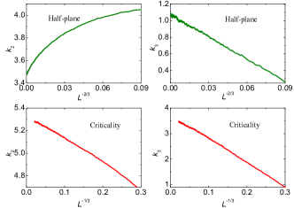
Figure 5: Leading order corrections of the second $k_{2}$ (left) and third $k_{3}$ (right) cumulants in the NSS model for a half-space versus $L^{-2/3}$ (top panels) and at the unbinding transition versus $L^{-1/3}$ (bottom panels).

We have shown that the NSS and the Anderson models in a half-plane undergo an unbinding transition as the hopping amplitude at the edge is varied. We show evidence that the analytical expressions for the conductance distribution functions and the scaling functions at the unbinding transitions in localized two-dimensional quantum systems are obtained from Eqs. (5-6). We have also studied the corresponding finite-size corrections. Similar unbinding transitions can occur in 3D systems when conduction through a surface or a line is favored. They may be relevant to the behavior of edge states.

- (1) P. J. Roberts, J. Phys.: Condens. Matter 4, 7795 (1992).
- (2) E. Abrahams, P. W. Anderson, D. C. Licciardello and T. V. Ramakrishnan, Phys. Rev. Lett. 42, 673 (1979).
- (3) B. Shapiro, Phil. Mag. B 56, 1031 (1987); A. Cohen, Y. Roth and B. Shapiro, Phys. Rev. B 38, 12125 (1988).
- (4) B. L. Altshuler, V. E. Kravtsov, I. E. Lerner in Chapter 10 in Mesoscopic Fluctuations in Solids Ed. B. L. Altshuler, P. A. Lee and R. A. Webb, Elsevier Science publishing B.V. 1991.
- (5) J. Prior, A. M. Somoza and M. Ortuño, Phys. Rev. B 72, 024206 (2005).
- (6) A. M. Somoza, M. Ortuño and J. Prior, Phys. Rev. Lett. 99, 116602 (2007).
- (7) C. A. Tracy and H. Widom, Commun. Math. Phys. 159, 151 (1994); 177, 727 (1996).
- (8) V. L. Nguyen, B. Z. Spivak and B. I. Shklovskii, Pis’ma Zh. Eksp. Teor. Fiz. 41, 35 (1985) [JETP Lett. 41, 42 (1985)]; Zh. Eksp. Teor. Fiz. 89, 11 (1985) [Sov. Phys.–JETP 62, 1021 (1985)].
- (9) E. Medina and M. Kardar, Phys. Rev. B 46, 9984 (1992); E. Medina, M. Kardar, Y. Shapir and X. R. Wang, Phys. Rev. Lett. 62, 941 (1989).
- (10) M. Kardar, G. Parisi and Y. C. Zhang, Phys. Rev. Lett. 56, 889 (1986).
- (11) M. Prähofer and H. Spohn, Phys. Rev. Lett. 84, 4882 (2000); J. Baik and E. M. Rains, J. Stat. Phys. 100, 523 (2000).
- (12) K. Johansson, Commun. Math. Phys. 209, 437 (2000).
- (13) J. Baik, P. A. Deift and K. Johansson, J. Amer. Math. soc. 12, 1119 (1999).
- (14) T. Sasamoto and H. Spohn, Phys. Rev. Lett. 104, 230602 (2010); Nucl. Phys. B 834, 523 (2010); J. Stat. Phys. 140, 209 (2010).
- (15) P. Calabrese, P. Le Doussal and A. Rosso, EPL 90, 20002 (2010). P. Calabrese and P. Le Doussal, Phys. Rev. Lett. 106, 250603 (2011) and J. Stat. Mech. P06001 (2012).
- (16) V. Dotsenko, EPL 90, 20003 (2010); J. Stat. Mech. P07010 (2010).
- (17) G. Amir, I. Corwin, J. Quastel, Comm. Pure Appl. Math 64, 466 (2011). I. Corwin, Random Matrices: Theory Appl. 01 1130001 (2012), arXiv:1106.1596.
- (18) T. Gueudre, P. Le Doussal, EPL 100 26006 (2012), arXiv:1208.5669.
- (19) T. Sasamoto, T. Imamura, J. Stat. Phys. 115 749 (2004), arXiv:cond-mat/0307011.
- (20) J. Baik, E. M. Rains in Random Matrix Models and Their Applications Eds: P. M. Bleher and A. R. Its, Cambridge Univ. Press 2001, arXiv:math/9910019.
- (21) M. Kardar, Phys. Rev. Lett. 55, 2235 (1985).
- (22) A. MacKinnon, Z. Phys. B 59, 385 (1985); J. A. Verges, Comput. Phys. Commun. 118, 71 (1999).
- (23) A. M. Somoza, M. Ortuño and J. Prior, Europhys. Lett. 70, 649 (2005).
- (24) J. Baik, arXiv:math/0504606.
- (25) K. A. Takeuchi, M. Sano, J. Stat. Phys. 147, 853 (2012), arXiv:1203.2530.
- (26) P. L. Ferrari, R. Frings, J. Stat. Phys. 144, 1123 (2011), arXiv:1104.2129.