Electrical Conductivity of an Anisotropic Quark Gluon Plasma : A Quasiparticle Approach

Abstract

The study of transport coefficients of strongly interacting matter got impetus after the discovery of perfect fluid ever created at ultrarelativistic heavy ion collision experiments. In this article, we have calculated one such coefficient viz. electrical conductivity of the quark gluon plasma (QGP) phase which exhibits a momentum anisotropy. Relativistic Boltzmann’s kinetic equation has been solved in the relaxation-time approximation to obtain the electrical conductivity. We have used the quasiparticle description to define the basic properties of QGP. We have compared our model results with the corresponding results obtained in different lattice as well as other model calculations. Furthermore, we extend our model to calculate the electrical conductivity at finite chemical potential.

PACS numbers: 12.38.Mh, 12.38.Gc, 25.75.Nq, 24.10.Pa

I Introduction

Transport coefficients are of particular interest to quantify the properties of strongly interacting matter created at relativistic heavy ion collisions (HIC) and these coefficients can be instrumental to study the critical properties of QCD medium. The fluctuations or external fields cause the system to depart from its equilibrium and a non-equilibrium system has been created for a brief time. The response of the system to such type of fluctuations or external fields is essentially described by transport coefficients eg. the shear and bulk viscosities, the speed of sound etc. In recent years a somewhat surprising result in the quark gluon plasma (QGP) story has occurred when the practitioners in this field tried to satisfy the collective flow data as obtained in collider experiments. In order to get the required collective flow in the framework of viscous hydrodynamics, the value of shear viscosity to entropy density ratio ($\eta/s$) comes out to be very small roma ; heinz ; kotun . The tiny value of $\eta/s$ indicates the discovery of most perfect fluid ever created in laboratory. This perfect fluid is described as strongly interacting quark gluon plasma lee ; guy ; shuryak ; hirano . Thus the study of various transport coefficients is a powerful tool to really understand the behaviour of the matter produced in the ultra relativistic heavy ion collision (uRHIC) experiments at RHIC and LHC.

Recently electrical conductivity has gained a lot of interest due to the strong electric field created in the collision zone of uRHIC experiments vgreco ; fraile ; greif . It has been observed that strong electric and magnetic fields are created in peripheral heavy ion collisions whose strength are roughly estimated as $eE=eB=m_{\pi}^{2}$(where $m_{\pi}$ is the mass of the pion) within proper time $1-2$ fm/c tuchin . This large electrical field can significantly affect the behaviour of the medium created in these collisions and the effect depends on the magnitude of electrical conductivity ($\sigma_{\rm{el}}$) of the medium. $\sigma_{\rm{el}}$ is responsible for the production of electric current generated by the quarks in the early stage of the collision. The value of $\sigma_{\rm{el}}$ would be of fundamental importance for the strength of Chiral Magnetic Effect fuku which is a signature of CP-violation in strong interaction. Further the electrical field in mass asymmetric collisions (e.g. $Cu$-$Au$ collisions etc.) has overall a preferred direction and thus generating a charge asymmetric flow whose strength is directly related to $\sigma_{\rm{el}}$ hongo . Furthermore, $\sigma_{\rm{el}}$ is related with the emission rate of soft photons kapusta accounting for their raising spectra turbide ; linnyk . Despite of the importance of electrical conductivity, it has been studied rarely in the literature for the QGP phase.

With the discovery of “most perfect fluid ever generated”, another important observation has been made that this fluid possesses momentum-space anisotropies in the local rest frame (LRF) strick ; strick1 . This has important implications for both dynamics and signatures of the QGP. Earlier it has been assumed a priori in the ideal hydrodynamics that the QGP is completely isotropic. However, recently dissipative hydrodynamics helps us to understand that the QGP created in ultrarelativistic heavy ion collisions has different longitudinal and transverse pressure. It has been shown heuristically in first-order Navier Stokes viscous hydrodynamics that the ratio of longitudinal pressure over the transverse pressure is: $P_{L}/P_{T}=(3\tau T-16\bar{\eta})/(3\tau T+8\bar{\eta})$, where $\bar{\eta}=\eta/s$ strick . Using the RHIC-like initial condition the value of $P_{L}/P_{T}$ comes out equal to $0.5$ and for LHC-like initial condition this ratio takes the value as $0.35$ strick . It has also been shown that there exists an anisotropy in $P_{L}$ versus $P_{T}$ in second-order Israel-Stewart viscous hydrodynamics. Several other groups who study the early-time dynamics of QCD within AdS/CFT framework have also shown the early-time pressure anisotropies and quote $P_{L}/P_{T}=0.31$ or smaller heller ; vander . In colour-glass condensate framework, the practitioners have found that the timescale for isotropization in classical Yang-Mills simulations is very long mac ; iancu . From these observations and findings one can certainly assumes that the momentum anisotropy produced in the medium created in heavy ion collisions lasts for at least $\tau\leq 2~{}fm/c$. Thus it is crucial to incorporate these momentum-space anisotropies in any phenomenological studies specifically for transport coefficients.

In this article our main motivation is to calculate the electrical conductivity of an anisotropic QGP phase using the Relativistic Boltzmann’s kinetic equation. We have used the quasiparticle description to define the basic properties of QGP since earlier we have shown that quasiparticle description provides the proper and realistic thermodynamical and transport behaviour of QGP phase pks ; pks1 . We want to provide the correct temperature dependence of $\sigma_{\rm{el}}$ since it is not yet established. Lattice calculations have obtained $\sigma_{\rm{el}}$ at few values of temperature and these estimates vary widely aamato ; ding ; aarts ; gupta . Thus it is necessary to provide a proper temperature dependence to electrical conductivity. We will also extend our calculation at finite quark chemical potential ($\mu_{q}$). This is important since there is no guidance at finite $\mu_{q}$ due to severe limitation of lattice calculations in this region. Very recently Berrehrah and collaborators have shown the variation of $\sigma_{\rm{el}}/T$ with respect to temperature at small but finite chemical potential in dynamical quasiparticle model (DQPM) berre .

Rest of the article is organized as follows : firstly we present the calculation of electrical conductivity in the isotropic case. In second subsection we introduce a momentum-space anisotropy in the distribution function of quarks and antiquarks and then derive the expression of $\sigma_{\rm{el}}$ for this anisotropic hot and/or dense QCD medium using Relativistic Boltzmann’s approach. In the third subsection we will provide a brief introduction about quasiparticle model. We further explain the importance of quasiparticle description of QGP in comparison to ideal description . Later we demonstrate results obtained in our model at zero $\mu_{q}$ and their comparison with the corresponding results obtained in lattice as well as in phenomenological calculations. We have also extended our model calculation at finite $\mu_{q}$. Finally we will give the summary and the conclusions drawn from this work.

II Description of Model

II.1 Electrical Conductivity for Isotropic System

The electric conductivity represents the response of the system to applied electric field. According to Ohm’s law, the spatial electric current (${\bf J}$) is directly proportional to the longitudinal component of the electric field ${\bf E}$ :

$${\bf J}=\sigma_{\rm{el}}{\bf E},$$ (1)

where the proportionality coefficient is known as electrical conductivity ($\sigma_{\rm{el}}$). One can write down the expression for four current ($J^{\mu}$) in a covariant form as:

$$J^{\mu}=\int\frac{d^{3}p}{(2\pi)^{3}E}p^{\mu}\{q~{}g~{}f(x,p)-{\bar{q}}~{}g~{}{\bar{f}}(x,p)\},$$ (2)

where $f(x,p)({\bar{f}(x,p)}$) and q (${\bar{q}}$) are the distribution function and electric charge for quark (anti-quark), respectively. Further $g$ is the degeneracy factor. Let us first assume the case of vanishing chemical potential i.e., $\mu_{q}=0$. In this case quark and anti-quark distribution functions will become identical, so Eq. (2) takes the following form:

$$J^{\mu}=2q_{{}_{f}}g_{{}_{f}}\int\frac{d^{3}p}{(2\pi)^{3}E}p^{\mu}f(x,p).$$ (3)

In the presence of infinitesimal external disturbance, the change in four current is :

$$\Delta J^{\mu}=2q_{{}_{f}}g_{{}_{f}}\int\frac{d^{3}p}{(2\pi)^{3}E}p^{\mu}\delta f(x,p),$$ (4)

where $\delta f$ is the change in distribution function due to external disturbance. One can obtain the $\delta f(x,p)$ by using the Relativistic Boltzmann Transport (RBT) equation, which is given by Yagi ; Cercignani :

$$p^{\mu}\partial_{\mu}f(x,p)+qF^{\alpha\beta}p_{\beta}\frac{\partial}{\partial p^{\alpha}}f(x,p)={\cal C}[f],$$ (5)

where $F^{\alpha\beta}$ is the electromagnetic field strength tensor and $C[f]$ is the collision integral, which in the relaxation-time approximation is given by :

$${\cal C}[f]\simeq-\frac{p^{\mu}u_{\mu}}{\tau}(f-f^{0}),\,\,(f-f^{0})=\delta f$$ (6)

where $\tau$ is the relaxation time and $f^{0}$ is the equilibrium distribution function. In this approximation, RBT equation becomes:

$$p^{\mu}\partial_{\mu}f(x,p)+qF^{\alpha\beta}p_{\beta}\frac{\partial}{\partial p^{\alpha}}f(x,p)=-\frac{p^{\mu}u_{\mu}}{\tau}\delta f$$ (7)

where $u^{\mu}$ is the fluid four velocity and in the local rest frame i.e., $u^{\mu}=(1,{\bf 0})$. The equilibrium quark distribution function at $\mu_{q}=0$ has the following form :

$$f^{0}(x,{\bf p};T)=\frac{1}{e^{E/T}+1},$$ (8)

where $E=\sqrt{{\bf p}^{2}+m^{2}}$.

Since we are interested only in electric field components of $F^{\alpha\beta}$, we take only two terms: $F^{0i}=-{\bf E}~{}\,\,and\,\,F^{i0}={\bf E}$. Thus the RBT equation (7) becomes:

$$-q\left(p_{0}{\bf E}\cdot\frac{\partial f^{0}}{\partial{\bf p}}-{\bf E}\cdot{\bf p}\frac{\partial f^{0}}{\partial p^{0}}\right)=-\frac{p^{0}}{\tau}\delta f,$$ (9)

where $\frac{\partial f^{0}}{\partial{\bf p}}$ can be solved by using the chain-rule and after differentiation we get the value of $\delta f$ as:

$$\delta f=q\tau\frac{{\bf E}\cdot{\bf p}}{p^{0}T}f^{0}(1-f^{0})$$ (10)

By substituting $\delta f$ in Eq. (4) we obtain the expression for $\sigma_{\rm{el}}$:

$$\sigma_{\rm{el}}^{\rm{iso}}=\frac{2}{T}\sum_{f}g_{{}_{f}}q_{{}_{f}}^{2}\int\frac{d^{3}p}{(2\pi)^{3}}\frac{{p}^{2}}{E^{2}}\tau_{{}_{f}}\times f_{{}_{f}}^{0}(1-f_{{}_{f}}^{0}),$$ (11)

where the subscript $f$ implies summation over the flavors. Here we have taken up, down and strange flavors only.

It is important to provide a connection between the calculation of electrical conductivity by thermal field theory and in Boltzmann’s kinetic approach. In an equilibrated system having volume $V$ and temperature $\beta^{-1}$, the zero frequency Green-Kubo green ; kubo formula for the electrical conductivity is given by the current-current autocorrelation

$$\sigma_{\rm{el}}=\beta V\int_{0}^{\infty}\langle j_{i}(0)j_{i}(t)\rangle dt,$$ (12)

where the repeated spatial-indices, $i$ do not imply summation. In the local rest frame of fluid, the electric current density can be read as :

$$j^{l}(t)=\frac{1}{V~{}N_{test}}\sum_{k=1}^{M}q_{k}\sum_{i=1}^{N_{k}}\left(\frac{p_{i}^{l}}{p_{i}^{0}}\right)_{t},$$ (13)

where $M$ is the number of particle-species and $N_{k}$ is the number of particles of $k$-th species. For all equivalent directions ($l$), $j_{l}(t)$ was obtained from Boltzmann Approach to Multi-parton Scatterings and then the autocorrelation function, $C(t)$ of the electric current density in equilibrium has been extracted greif . For example, the variance, $C(0)$ has been computed analytically

$$C(0)=\frac{1}{3V}\sum_{k=1}^{M}q_{k}^{2}n_{k},$$ (14)

which finally gives the expression for $\sigma_{\rm{el}}$ :

$$\sigma_{\rm{el}}=\frac{1}{3T}\sum_{k=1}^{M}q_{k}^{2}n_{k}\tau~{},$$ (15)

which is nothing but the non-relativistic Drude’s formula to calculate the $\sigma_{\rm{el}}$. Similarly one can show that the expression for $\sigma_{\rm{el}}$ obtained by solving relativistic Boltzmann kinetic equation (see Eq. (11)) can also be approximated as Drude’s formula assuming small electric field and no cross effects between heat and electrical conductivity greif .

At finite quark-chemical potential ($\mu_{q}\neq 0$), the distribution function for quark and anti-quark will be different. For quarks :

$$f^{0}_{f}(x,{\bf p};T,\mu_{q})=\frac{1}{e^{(E-\mu^{q}_{f})/T}+1},$$ (16)

and for antiquarks :

$${\bar{f}^{0}_{f}}(x,{\bf p};T,\mu_{q})=\frac{1}{e^{(E+\mu^{q}_{f})/T}+1}.$$ (17)

One can then generalize the expression for electrical conductivity in an isotropic medium for $\mu_{q}\neq 0$ as follows :

$$\sigma_{\rm{el}}^{\rm{iso}}(\mu_{q}\neq 0) = \frac{1}{T}\sum_{f}g_{f}q_{f}^{2}\int\frac{d^{3}p}{{(2\pi)}^{3}}\frac{{p}^{2}}{E^{2}}$$ (18)

$$\times \left[\tau_{{}_{f}}f_{{}_{f}}^{0}(1-f_{{}_{f}}^{0})+\tau_{\bar{{}_{f}}}{\bar{f_{{}_{f}}}^{0}}(1-{\bar{f}_{{}_{f}}^{0}})\right].$$

II.2 Electrical Conductivity for Anisotropic System $\xi\neq 0$

The introduction of an anisotropic distribution function is needed to properly describe the QGP created in heavy ion collisions dum1 ; dum2 . Partons are produced from the incoming colliding nuclei just after the collision at proper time $\tau=\tau_{0}\approx Q_{s}^{-1}$, it can be assumed that the newly produced partons follow an isotropic (but not necessary an equilibrium) momentum distribution. Here $Q_{s}$ is the gluon saturation scale. The early-time physics is mainly governed by the hard gluons with the momentum at the saturation scale which have very large occupation numbers of order $1/\alpha_{s}$ ($\alpha_{s}<<1$) gribov ; mueller ; blaiz . For $\tau>Q_{s}^{-1}$, the hard gluons would follow the straight-line trajectories and isolate themselves in beam direction as if no any interaction exists. As a result, the longitudinal expansion causes the medium to become much colder in the longitudinal direction than the transverse direction, ie. $p_{\perp}>>p_{z}\sim 1/\tau$ and a local momentum anisotropy appears.

The anisotropic distribution can be obtained by stretching or squeezing an isotropic one along a certain direction, thereby preserving a cylindrical symmetry in momentum space. In particular, the anisotropic distribution relevant for HICs can be approximated by removing particles with the large momentum component along the direction of anisotropy, ${\bf n}$ as roma1 ; roma2 :

$$f_{\rm{aniso}}({\mathbf{p}})=f_{iso}\left(\sqrt{p^{2}+\xi({\mathbf{p}}\cdot{\mathbf{n}})^{2}}\right),$$ (19)

where $f_{iso}$ is an arbitrary isotropic distribution function and $\xi$ is the anisotropic parameter and is generically defined as:

$$\xi=\frac{\langle{\bf p}_{T}^{2}\rangle}{2\langle p_{L}^{2}\rangle}-1,$$ (20)

where $p_{L}={\mathbf{p}}.{\mathbf{n}}$ and ${\mathbf{p}}_{T}={\mathbf{p}}-{\mathbf{n}}({\mathbf{p}}.{\mathbf{n}})$ are the components of momentum parallel and perpendicular to ${\mathbf{n}}$, respectively. There have been significant advances in the dynamical models used to simulate plasma evolution with the momentum-space anisotropies Martinez:2010sd-12tu ; Martinez:PRC852012 ; Ryblewski:2010bs ; Ryblewski:2012rr ; Florkowski:2010cf . Recently two of us have investigated the effects of anisotropy on the quarkonia states by the leading-anisotropic correction to the potential at T=0 lata:PRD2013 ; lata:PRD2014 .

If $f_{iso}$ is a thermal ideal-gas distribution and $\xi$ is small then $\xi$ is also related to the shear viscosity of the medium via one-dimensional Bjorken expansion in the Navier-Stokes limit asa ::

$$\xi=\frac{10}{T\tau}\frac{\eta}{s},$$ (21)

In an expanding system, non-vanishing viscosity implies finite-momentum relaxation rate and therefore an anisotropy of the particle momenta appears. For $\eta/s=0.1-0.3$ and $\tau T=1-3$, one finds that $\xi=1$.

As we have explained, hot QCD medium due to expansion and non zero viscosity, exhibits a local anisotropy in momentum space, and the quark distribution function (or Fermi-Dirac distribution function) takes the following form for $\mu_{q}=0$:

$$f_{\rm{aniso}}(x,{\bf p};T)=\frac{1}{e^{(\sqrt{{\bf p}^{2}+\xi({\bf p}.{\bf n})^{2}+m^{2}})/T}+1}.$$ (22)

For weakly anisotropic systems ($\xi<<1$), one can expand the quark distribution function as follows :

$$f_{\rm{aniso}}(x,{\bf p};T) = \frac{1}{e^{E/T}+1}-\frac{\xi}{2ET}({\bf{p\cdot n}})^{2}\frac{e^{E/T}}{(e^{E/T}+1)^{2}},$$ (23)

$$= f^{0}-\frac{\xi}{2ET}{({\bf p}\cdot{\bf n})}^{2}{f^{0}}^{2}e^{E/T},$$

where ${\bf p}$ $\equiv$ $(p\sin\theta\cos\phi,p\sin\theta\sin\phi,p\cos\theta)$ and ${\bf n}$ $\equiv$ $(\sin\alpha,0,\cos\alpha)$. $\alpha$ is the angle between ${\bf p}$ and ${\bf n}$. After substituting the anisotropic distribution function in Eq. (11), the expression of electrical conductivity in anisotropic medium system is modified as:

$$\sigma_{\rm{el}}^{\rm{aniso}}=g_{f}\frac{2~{}q_{f}^{2}}{T}\int\frac{d^{3}p}{(2\pi)^{3}}\frac{{p}^{2}}{E^{2}}\tau_{f}f_{aniso}(1-f_{aniso})$$ (24)

On neglecting the higher-order distribution function (e.g., $f_{0}^{3}$ etc.) we get the expression for electrical conductivity as:

$$\sigma_{\rm{el}}^{\rm{aniso}} = g_{f}\frac{2~{}q_{f}^{2}}{T}\int\frac{d^{3}p}{(2\pi)^{3}}\frac{{p}^{2}}{E^{2}}\tau_{f}f^{0}(1-f^{0})$$

$$- \xi g_{f}\frac{q_{f}^{2}}{T^{2}}\int\frac{d^{3}p}{(2\pi)^{3}}\frac{{p}^{2}}{E^{3}}\tau_{f}(f^{0})^{2}e^{E/T}({\bf{p\cdot n}})^{2}$$

Now using the definition of $\mathbf{p}$ and $\mathbf{n}$, and integrating over $\theta$ and $\phi$, we get the electrical conductivity in anisotropic medium, after summing over the flavours ($f$)

$$\sigma_{\rm{el}}^{\rm{aniso}}(\mu_{q}=0) = \frac{1}{\pi^{2}T}\sum_{f}g_{{}_{f}}q_{{}_{f}}^{2}\int dp\frac{{p}^{4}}{E^{2}}\tau_{{}_{f}}f_{{}_{f}}^{0}(1-f_{{}_{f}}^{0})$$ (26)

$$- \xi\frac{1}{6\pi^{2}T}\sum_{f}g_{{}_{f}}q_{{}_{f}}^{2}\int dp\frac{{p}^{6}}{E^{3}}\tau_{{}_{f}}(f_{{}_{f}}^{0})^{2}e^{E/T}$$

$$= \sigma_{\rm{el}}^{\rm{iso}}-\xi A,$$

where the anisotropic term, $A$ is given by

$$A=\frac{1}{6\pi^{2}T}\sum_{f}g_{{}_{f}}q_{{}_{f}}^{2}\int dp\frac{{p}^{6}}{E^{3}}\tau_{{}_{f}}(f_{{}_{f}}^{0})^{2}e^{E/T}$$ (27)

Like in the isotropic medium, we can generalize the electrical conductivity in an anisotropic medium for $\mu_{q}\neq 0$:

$$\sigma_{\rm{el}}^{\rm{aniso}}(\mu_{q}\neq 0) = \frac{1}{2\pi^{2}T}\sum_{f}g_{{}_{f}}q_{{}_{f}}^{2}\int dp\frac{{p}^{4}}{E^{2}}$$

$$\times \left[\tau_{{}_{f}}f_{{}_{f}}^{0}(1-f_{{}_{f}}^{0})+\tau_{\bar{{}_{f}}}{\bar{f}_{{}_{f}}^{0}}(1-{\bar{f}_{{}_{f}}^{0}})\right]$$

$$- \xi\frac{1}{12\pi^{2}T^{2}}\sum_{f}g_{{}_{f}}q_{{}_{f}}^{2}\int dp\frac{{p}^{6}}{E^{3}}$$

$$\times \left[e^{(E-\mu^{q}_{f})/T}\tau_{{}_{f}}(f_{{}_{f}}^{0})^{2}+e^{(E+\mu^{q}_{f})/T}\tau_{\bar{{}_{f}}}({\bar{f}_{{}_{f}}^{0}})^{2}\right],$$

where $f_{{}_{f}}^{0}$ and ${\bar{f}_{{}_{f}}^{0}}$ acquire the form as given in Eq. (16) and (17), respectively.

II.3 Quasiparticle Model: Effective Masses and Relaxation Times

Quasiparticles are the thermal excitations of the interacting quarks and gluons retaining the quantum numbers of the real particles, i.e., the quarks and gluons. In quasiparticle models pe.1 , QGP is described by the system of ’massive’ noninteracting quasiparticles where the mass of these quasiparticles is temperature-dependent and arises because of the interactions of quarks and gluons with the surrounding matter in the medium. The effective mass of these quasiparticles is given by pks :

$$m_{{}_{f}}^{2}=m_{0,f}^{2}+\sqrt{2}m_{0,f}m_{th,f}+m_{th,f}^{2},$$ (29)

where $m_{0,f}$ is the current mass of the flavour, $f$ and $m_{th,f}$ is the thermal mass of the flavour, $f$, which is given by

$$m_{th,f}^{2}=\frac{g^{2}(T)T^{2}}{6}\left(1+\frac{(\mu^{q}_{{f}})^{2}}{\pi^{2}T^{2}}\right).$$ (30)

Here $g^{2}$ is the QCD running coupling constant which in two-loop has following form laine ; agotiya :

$$\alpha_{S}(T,~{}\mu_{q}) = \frac{g^{2}(T,~{}\mu_{q})}{4\pi}=\frac{6\pi}{\left(33-2N_{f}\right)\ln\left(\frac{T}{\Lambda_{T}}\sqrt{1+a\frac{\mu_{q}^{2}}{T^{2}}}\right)}$$

$$\times \left(1-\frac{3\left(153-19N_{f}\right)}{\left(33-2N_{f}\right)^{2}}\frac{\ln\left(2\ln\frac{T}{\Lambda_{T}}\sqrt{1+a\frac{\mu_{q}^{2}}{T^{2}}}\right)}{\ln\left(\frac{T}{\Lambda_{T}}\sqrt{1+a\frac{\mu_{q}^{2}}{T^{2}}}\right)}\right),$$

where $\Lambda_{T}$ is the QCD scale-fixing parameter which characterizes the strength of the interaction. It originates from the lowest non-zero Matsubara modes vuo . Here parameter $a$ is equal to $\frac{1}{\pi^{2}}$.

In Eqs. (18) and (II.2), $\tau_{f}$ is the collision time for which we use the following expressions for quarks (anti-quarks) from Ref. hosoya :

$$\tau_{q(\bar{q})}=\frac{1}{15\alpha_{s}^{2}T{}log\left(\frac{1}{\alpha_{s}}\right)\left(1+0.06N_{F}^{eff}\right)},$$ (32)

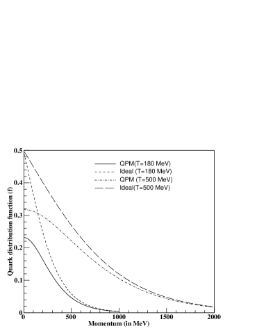
Figure 1: Variation of QPM and ideal distribution function with respect to momentum at two different temperatures. Solid and dash-dotted curve represents the light quark distribution function in QPM at $T=180$ and $500$ MeV, respectively. Similarly short-dashed and long-dashed curve shows the corresponding results in ideal description.

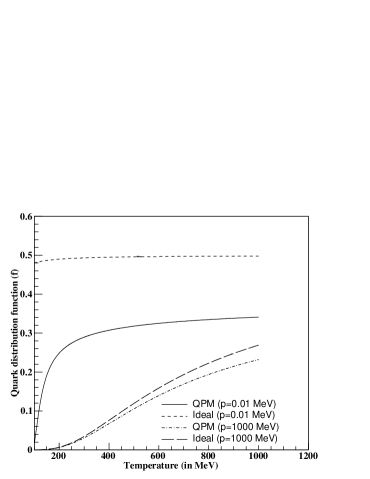
Figure 2: Variation of QPM and ideal distribution functions with respect to temperature at two different momentum.Solid and dash-dotted curve represents the light quark distribution function in QPM at $p=0.01$ and $1000$ MeV, respectively. Similarly short-dashed and long-dashed curve shows the corresponding results in ideal description.

where $N_{F}^{\rm{eff}}$ is the number of effective flavour degrees of freedom.
Before going to the electrical conductivity results, we want to just provide the difference between the ideal description (where the mass consists of only the current mass) and the quasiparticle description (where the mass consists of current mass along-with a thermally generated mass) of QGP. To understand the crucial difference between these two descriptions, it is better to plot the occupation probability or distribution function in both descriptions. In Fig. 1, we have shown the variation of QPM distribution function for light quarks ($u$ and/or $d)$ with respect to momentum at two different temperatures $T=180$ and $500$ MeV. We further compare these results with the corresponding ideal distribution functions where we use only the current mass of the quarks in the mass term and there is no any thermal contribution. We observe that at low momentum the difference between QPM and ideal description is large. The QPM occupation probability is low in comparison to ideal case and thus we can indirectly say that the number density will also be small. However, at higher momentum, both picture give the same distribution function. Similarly, Fig. 2 demonstrates the variation of QPM distribution function with respect to temperature at two different momentum $p=0.01$ MeV (low momentum) and $1000$ MeV (high momentum). We have also plotted the corresponding ideal distribution function for comparison. Here we observed that the QPM distribution function or QPM occupation probability is small in comparison to ideal case at low momentum and this difference increases as we move from higher temperatures towards lower temperature. However, at higher momentum the difference between QPM and ideal distribution function is quite insignificant over the entire temperatures range considered by us. As we know from non-relativistic Drude’s formula that the electrical conductivity is directly proportional to the number density which is nothing but the integration of distribution function over momentum space at any particular temperature. Therefore one can understand the usefulness of QPM description in describing the thermodynamical and transport properties of QGP specially near the critical temperature ($T_{c}$).

III Results and Discussions

Figure 3: Variation of ratio of electrical conductivity to temperature ($\sigma_{\rm{el}}^{\rm{aniso}}/T$) with respect to temperature at different values of anisotropy parameter $\xi=0.0,~{}0.3$ and $0.6$ and they are shown in the plot by solid, dashed and dash-dotted line, respectively. Green points are the results as obtained from dynamical quasiparticle model (DQPM) in Ref. cassing . All other symbols are the data points obtained from various lattice calculations aamato ; ding ; aarts ; gupta .

In Fig. 3, we present the variation of ratio of electrical conductivity to temperature ($\sigma_{\rm{el}}^{\rm{aniso}}/T$) with respect to temperature at $\mu_{q}=0$ for an anisotropic QGP. For weakly anisotropic system, we choose three constant values of $\xi$ as $0.0,~{}0.3$ and $0.6$, where $\xi=0.0$ represents $\sigma_{\rm{el}}/T$ in isotropic case as mentioned in Eq. (11). We have compared our model results with the corresponding results obtained in various lattice calculations  aamato ; ding ; aarts ; gupta . We further compared our model results with the $\sigma_{\rm{el}}/T$ obtained in DQPM model cassing . We observe that $\sigma_{\rm{el}}^{\rm{aniso}}/T$ increases monotonically with temperature starting from a lower value at $T=T_{c}$, where $T_{c}$ is the crossover temperature for the transition from QGP to hadron gas (HG). Further we observe that as the anisotropy increases from $0.0$ to $0.6$, the value of $\sigma_{\rm{el}}/T$ decreases for all the temperatures. $\sigma_{\rm{el}}^{\rm{aniso}}/T$ satisfies the lattice results well when the anisotropy parameter has a value equal to $0.6$. The results obtained from DQPM overestimate the value of $\sigma_{\rm{el}}/T$ as compared to the lattice as well as our model calculations. However, we cannot say at this moment the exact status of any model calculations since the lattice results are distributed over a wide range.

Figure 4: Variation of ratio of electrical conductivity to temperature ($\sigma_{\rm{el}}^{\rm{aniso}}/T$) with respect to temperature at two different values of anisotropy parameter $\xi=0.0$ and $0.6$ for quark chemical potential $\mu_{q}=0$ and $\mu_{q}=200~{}MeV$.

Fig.4 represents the variation of $\sigma_{\rm{el}}^{\rm{aniso}}/T$ with respect to temperature at quark chemical potential $\mu_{q}=200~{}MeV$ and compare them with our model results at $\mu_{q}=0~{}MeV$. Here we have shown the results for two different values of $\xi$ equal to $0.0$ and $0.6$. Solid and long-dashed curve demonstrate the $\sigma_{\rm{el}}^{\rm{aniso}}$ at $\mu_{q}=0.0$ for $\xi=0.0$ and $0.6$, respectively. Short-dashed and dash-dotted curve show the results at $\mu_{q}=200$ MeV for $\xi=0.0$ and $0.6$, respectively. At large temperatures we found that $\sigma_{\rm{el}}^{\rm{aniso}}/T$ at finite $\mu_{q}$ remains same as in the case of zero $\mu_{q}$. However, the value of $\sigma_{\rm{el}}^{\rm{aniso}}/T$ becomes large for finite $\mu_{q}$ in comparison to the value at $\mu_{q}=0~{}MeV$ as the temperature decreases below $T=4T_{c}$. This behaviour is quite consistent with the results obtained in a very recent DQPM calculations at finite $\mu_{q}$ berre .

In summary we have studied the behaviour of electrical conductivity for QGP phase in the framework of relativistic Boltzmann’s kinetic equation using relaxation time approximation. In this work we describe the QGP as a system of quasiparticles having temperature and chemical potential dependent mass along with their rest masses. Firstly we derive the expression to calculate $\sigma_{\rm{el}}$ in an isotropic medium. Later a momentum anisotropy in the distribution function of quarks and anti-quarks has been introduced and taking the leading order contribution in distribution function we have obtained $\sigma_{\rm{el}}$ in an anisotropic medium which is equal to the $\sigma_{\rm{el}}^{\rm{iso}}$ minus the correction factor due to momentum anisotropy. We have plotted $\sigma_{\rm{el}}^{\rm{aniso}}/T$ for different values of $\xi$ which is equal to $0.0,~{}0.3$ and $0.6$. We have compared our model results with the corresponding results obtained in various lattice results and found a reasonable agreement between them for certain value of $\xi$. Further, we have plotted our model expectations for $\sigma_{\rm{el}}^{\rm{aniso}}/T$ at $\mu_{q}=200~{}MeV$ and compare them with the model results obtained at zero chemical potential. Both in isotropic as well as in anisotropic case, we find the similar behaviour as observed in DQPM calculations berre i.e., increase in the value of $\sigma_{\rm{el}}/T$ with increase in quark chemical potential near $T_{c}$. At very high temperatures ($T\sim 8-10T_{c}$), the difference between $\mu_{q}=0.0$ and $\mu_{q}=200~{}MeV$ case is very small. These calculations are done in a static system when there is no any proper time dependence has been given to the anisotropy parameter. However, in realistic situation, $\xi$ varies with the proper time starting from the initial proper time up to a time when the system becomes isotropic and $\xi$ becomes zero. Thus one has to incorporate a proper time dependence to the anisotropy parameter. Work in this direction is in progress and will be presented elsewhere.

IV Acknowledgments

The authors are thankful for financial assistance from Council of Scientific and Industrial Research (No. CSR-656-PHY), Government of India.

References

- (1) P. Romatschke and U. Romatschke, Phys. Rev. Lett. 99, 172301 (2007); B. Schenke, S. Jeon and C. Gale, Phys. Rev. C 82, 014903 (2010).
- (2) U. Heinz, P.F. Kolb, Nuclear Phys. 702 (2002).
- (3) P. K. Kovtun, D. T. Son and A. O. Starinets, Phys. Rev. Lett. 94, 111601 (2005).
- (4) T.D. Lee, Nuclear Phys. 750, 1 (2005).
- (5) M. Gyulassy, L. Mclerran, Nuclear Phys. 750, 30 (2005).
- (6) E.V. Shuryak, Nuclear Phys. 750, 64 (2005).
- (7) T. Hirano, M. Gyulassy, Nuclear Phys. 769, 71 (2006).
- (8) A. Puglisi, S. Plumari and V. Greco, arXiv:1407.2259v1[hep-ph] (2014).
- (9) D. Fernandez-Fraile and A. Gomez Nicola, Phys. Rev. D 73, 045025 (2006).
- (10) M. Greif, I. Bouras, C. Greiner, Z. Xu, Phys. Rev. D 90, 094014 (2014).
- (11) K. Tuchin, Advances in High Energy Physics 2013, 490495 (2013).
- (12) K. Fukushima, D. E. Kharzeev and H. J. Warringa, Phys. Rev. D 78, 074033 (2008).
- (13) Y. Hirono, M. Hongo, T. Hirano, arXiv:1211.1114[hep-ph] (2012).
- (14) J. Kapusta, Finite-temperature field theory, Cambridge monographs on mathematical physics, Cambridge University Press (1993).
- (15) S. Turbide, R. Rapp, and C. Gale, Phys. Rev. C 69, 014903 (2004).
- (16) O. Linnyk, W. Cassing and E. Bratkovskaya, Phys. Rev. C 89, 034908 (2014).
- (17) M. Strickland, arXiv:1401.1188v1[nucl-th] (2014).
- (18) M. Strickland, Nucl. Phys. A 926, 92 (2014); arXiv: 1312.2285[hep-ph] (2013).
- (19) M. P. Heller, R. A. Janik, and P. Witaszczyk, Phys. Rev. Lett. 108, 201602 (2012).
- (20) W. vander Schee, P. Romatschke, and S. Pratt, Phys. Rev. Lett. 111, 222302 (2013).
- (21) L. D. McLerran, and R. Venugopalan, Phys. Rev. D 49, 2233 (1994).
- (22) E. Iancu and R. Venugopalan, hep-ph/0303204 (2003).
- (23) P. K. Srivastava, S. K. Tiwari and C. P. Singh, Phys. Rev. D 82, 014023 (2010).
- (24) P. K. Srivastava and C. P. Singh, Phys. Rev. D 85, 114016 (2012).
- (25) A. Amato, G. Aarts, C. Allton, P. Giudice, S. Hands, and J. Skullerud, Phys. Rev. Lett. 111, 172001 (2013).
- (26) H. -T. Ding, A. Francis, O. Kaczmarek, F. Karsch, E. Laermann, W. Soeldner, Phys. Rev. D 83, 034504 (2011).
- (27) G. Aarts, C. Allton, J. Foley, S. Hands, S. Kim, Phys. Rev. Lett. 99, 022002 (2007).
- (28) S. Gupta, Phys. Lett. B 597, 57 (2004).
- (29) H. Berrehrah, E. Bratkovskaya, W. Cassing and R. Marty, arXiv:1412.1017v1[hep-ph] (2014).
- (30) K. Yagi, T. Hatsuda, Y. Miake, Quark-Gluon Plasma: from big bang to little bang, Cambridge University Press, 2005.
- (31) C. Crecignani and G. M. Kremer, The Relativistic Boltzmann Equation: Theory and Applications, Boston; Basel; Berlin: Birkhiiuser, 2002.
- (32) M. S. Green, J. Chem. Phys. 20, 1281 (1952).
- (33) R. Kubo, J. Phys. Soc. Jpn. 12, 570 (1957).
- (34) A. Dumitru, Y. Guo and M. Strickland, Phys. Lett. B 662, 37 (2008).
- (35) A. Dumitru, Y. Guo, A. Mocsy and M. Strickland, Phys. Rev. D 79, 054019 (2009).
- (36) L. V. Gribov, E. M. Levin and M. G. Ryskin, Phys. Rept. 100, 1 (1983).
- (37) A. H. Mueller and J.-W. Qiu, Nucl. Phys. B 268, 427 (1986).
- (38) J. P. Blaizot and A. H. Mueller, Nucl. Phys. B 289, 847 (1987).
- (39) P. Romatschke and M. Strickland, Phys. Rev. D 68, 036004 (2003).
- (40) P. Romatschke and M. Strickland, Phys. Rev. D 70, 116006 (2004).
- (41) M. Martinez and M. Strickland, Nucl. Phys. A 856, 68 (2011); Nucl. Phys. A 848, 183 (2010)
- (42) M. Martinez, R. Ryblewski, and M. Strickland, Phys. Rev. C 85, 064913 (2012).
- (43) R. Ryblewski, and W. Florkowski, J. Phys. G 38, 015104 (2011); Euro. Phys. J. C 71, 1761 (2011).
- (44) R. Ryblewski, W. Florkowski, Phys. Rev. C 85, 064901 (2012);W. Florkowski, R. Ryblewski, and M. Strickland, Phys. Rev. D 86, 085023 (2012).
- (45) W. Florkowski and R. Ryblewski, Phys. Rev. C 83, 034907 (2011).
- (46) L. Thakur, N. Haque, U. Kakade, and Binoy Krishna Patra, Phys. Rev. D 88, 054022 (2013).
- (47) L. Thakur, U. Kakade, and Binoy Krishna Patra, Phys. Rev. D 89, 094020 (2014).
- (48) A. Peshier, B. Kampfer, O. P. Pavlenko and G. Soff, Phys. Lett. B 337, 235 (1994)
- (49) M. Asakawa, S. A. Bass, and B. Muller, Prog. Theor. Phys. 116, 725 (2007).
- (50) M. Laine, Y. Schroder, J. High. Energy Phys. 0503, 067 (2005).
- (51) V. Agotiya, L. Devi, U. Kakade and B. K. Patra, Int. J. Mod. Phys. A 1250009 (2012).
- (52) A. Vuorinen, arXiv:hep-ph/0402242.
- (53) A. Hosoya and K. Kajantie, Nucl. Phys. B 250, 666 (1985).
- (54) W. Cassing, O. Linnyk and T. Steinert, Phys. Rev. Lett. 110, 182301 (2013).