Abstract

Motivated by recent cosmological observations of a possibly unsuppressed primordial tensor component $r$ of inflationary perturbations, we reanalyse in detail the 5D conformal SUGRA originated natural inflation model of Ref. [1]. The model is a supersymmetric variant of 5D extra natural inflation, also based on a shift symmetry, and leads to the potential of natural inflation. Coupling the bulk fields generating the inflaton potential via a gauge coupling to the inflaton with brane SM states we necessarily obtain a very slow gauge inflaton decay rate and a very low reheating temperature $T_{r}\stackrel{{\scriptstyle<}}{{{}_{\sim}}}{\cal O}(100)$ GeV. Analysis of the required number of e-foldings (from the CMB observations) leads to values of $n_{s}$ in the lower range of present Planck 2015 results. Some related theoretical issues of the construction, along with phenomenological and cosmological implications, are also discussed.

1 Introduction

Inflation solves the problems of early cosmology in a natural way [2] and besides that produces a primordial fluctuation spectrum [3] which allows to discuss structure formation successfully. In detailed models (i) a sufficient number of $\operatorname{e}$-folds for the inflationary phase has to be produced, (ii) guided by bounds presented recently by the Planck Collaboration [4], the cosmic background radiation and a spectral index $n_{s}=0.968\pm 0.006$ should be generated. And (iii), the normalization of fluctuations has to be reproduced. Rather flat potentials for the inflaton field lead to the “slow roll” needed for (i). Such potentials appear naturally in (tree level) global supersymmetric models; higher loop corrections can be controlled, but the inclusion of supergravity easily produces an inflaton mass of the order of the Hubble scale.

In models with an extra dimension the fifth component of a $\text{U}(1)$ gauge field entering in a Wilson loop operator can act as an inflaton field of pseudo Nambu-Goldstone type which is protected against gravity corrections and avoids a transplanckian scale [6], [7], present in the original model of “natural inflation” [8]. We have presented such a model [1] based on 5D conformal SUGRA on an orbifold $\text{S}^{1}\!/\mathbb{Z}_{2}$ with a predecessor based on global supersymmetry with a chiral “radion” multiplet on a circle in the fifth dimension  [9]. We also made the interesting observation that a spectral index $n_{\text{s}}\sim 0.96$ as observed recently [different from a value very close to one usually obtained in straightforward SUSY hybrid inflation [11]], is obtained rather generically in gauge inflation. Actually, in the supersymmetric formulation we have a complex scalar field which besides the gauge inflaton $A_{5}^{1}$ contains a further “modulus” field $M^{1}$ which also might allow for successful inflation [1]. The main difference between the two inflation types is that gauge inflation leads to a large tensor to scalar ratio $r(\sim 0.12$ in [1]) whereas modulus inflation leads to very small $r(\stackrel{{\scriptstyle<}}{{{}_{\sim}}}10^{-4}$ in [1]). Recently the BICEP2 data [12] gave strong indication of a large ratio $r=0.2^{+0.07}_{-0.05}$ though recent joint analysis of BICEP2/Keck and Planck [13] gave a reduced upper bound $r\stackrel{{\scriptstyle<}}{{{}_{\sim}}}0.12$, with the likelihood curve for $r$ having a maximum for $r\simeq 0.05$. Because of this, we here consider the gauge inflation of ref. [1] again with particular emphasis on the required length of inflation. The well known $62$ $e$-folds solving the horizon problem will turn out to require a substantial expansion during the reheating period within the natural inflation scenario emerged from 5D SUGRA.

Let us present the organization of the paper and summarize some of the results. In Sec. 2 we perform a detailed analysis of natural inflation with $\cos$-type potential. For the calculation of the spectral index $n_{s}$ and the tensor to scalar ratio $r$, we use a second order approximation with respect to slow roll (SR) parameters. Since these quantities ($n_{s},r$) are determined at the point where the SR parameters are tiny, this approximation is sufficient for all practical purposes. However, near the end of the inflation, when SR breaks down, we perform an accurate numerical determination of the point via the condition $\epsilon_{H}=1$ on the Hubble slow roll parameter (see [15]-[17] for definitions). This is needed to compute, with desired precision, the number of $e$-foldings ($N_{e}^{\rm inf}$) before the end of the inflation. We carry out our analysis by using recent fresh data [4] for $n_{s}$, $N_{e}$, the amplitude of curvature perturbations and bounds for $r$ [13]. Our results are in agreement with a recent analysis of natural inflation by Freese and Kinney (see $2^{\rm nd}$ citation in [8]). For various cases we have also calculated the reheat temperature, which we use later on for contrasting with our 5D SUGRA emerged inflation scenario requiring a very low reheat temperature.

In Sec. 3 and Appendix A we shortly review our model of ref. [1] in a more self-contained way and discuss how natural inflation emerges from $5$D SUGRA. Using a superfield formulation, we do not need to go into the details of the component expressions in conformal 5D SUGRA of Fujita, Kugo and Ohashi (FKO) [18]. Indeed this emerged from our discussion [19, 20] (see also Ref. [23]) bringing the 5D conformal SUGRA formulation closer to the 4D global SUSY language [20]. We concentrate here on gauge inflation, i.e. on the case $M^{1}=0$ (stabilized moduli in the origin or a choice of initial conditions). In section 3, discussing the realization of natural inflation within 5D SUGRA, we present a new mechanism for inflaton decay, which eventually leads to the reheat of the Universe. Note that, besides a specific string theory realization [25], the inflaton decay and reheating has never been discussed before in the context of natural inflation. We show that the inflaton’s slow decay is a natural consequence of the 5D construction (with consistent UV completion), being realized by couplings of the heavy bulk supermultiplets generating the inflaton potential through their gauge coupling with brane SM states. Since the inflaton decay proceeds by 4-body decay and the decay width is strongly suppressed by the 2-nd power of the tiny $U(1)$ gauge coupling constant (of the gauge inflaton-charged fields) and a relatively small inflaton mass coupled to the intermediate bulk fields, a strong suppression of the reheat temperature $T_{r}$ comes out naturally. Our 5D SUGRA construction allows us to make an estimate $T_{r}\sim 0.34\rho_{reh}^{1/4}\sim|\lambda|^{2}\times 100$ GeV (where $\lambda\stackrel{{\scriptstyle<}}{{{}_{\sim}}}1$ is a brane Yukawa coupling). At the end of Sec. 3 we show that, by the parameters we are dealing with, preheating is excluded within the considered scenario.

Appendix A discusses the Kaluza-Klein spectrum of the fields involved, as well as the SUSY breaking effects for brane fields. We also perform a derivation of higher dimensional operators involving the inflaton $\phi_{\Theta}$ and light (MSSM) states relevant for the inflaton decay. As it turns out, the dominant decay channel is $\phi_{\Theta}\to llhh$ (with $l$ and $h$ denoting SM lepton and Higgs doublets respectively). Sec. 4 includes a discussion and concluding remarks about some related issues.

2 Natural inflation

In this section we analyse inflation with the potential of natural inflation [8] given by:

$${\cal V}={\cal V}_{0}\left(1+\cos(\alpha\phi_{\Theta})\right)~{},$$ (1)

where $\phi_{\Theta}$ is a canonically normalized real scalar field of inflation. In the concrete scenario of Ref. [1], we focus later on, the inflaton originates from a $5$D gauge superfield, while the parameters/variables of (1) are derived through the underlying 5D SUGRA. See Eqs. (24), (25), (A.17) and also the comment underneath Eq. (A.17).

The slow roll parameters (”VSR” - derived through the inflaton potential) are given by

$$\epsilon=\frac{M_{Pl}^{2}}{2}\left(\frac{{\cal V}^{\prime}}{{\cal V}}\right)^{2}=\frac{(M_{Pl}\alpha)^{2}}{2}\tan^{2}\frac{\alpha\phi_{\Theta}}{2}$$

$$\eta=M_{Pl}^{2}\frac{{\cal V}^{\prime\prime}}{{\cal V}}=\frac{(M_{Pl}\alpha)^{2}}{2}\left(\tan^{2}\frac{\alpha\phi_{\Theta}}{2}-1\right)=\epsilon-\frac{1}{2}(M_{Pl}\alpha)^{2}~{},$$

$$\xi=M_{Pl}^{4}\frac{{\cal V}^{\prime}{\cal V}^{\prime\prime\prime}}{{\cal V}^{2}}=-(M_{Pl}\alpha)^{4}\tan^{2}\frac{\alpha\phi_{\Theta}}{2}=-2(M_{Pl}\alpha)^{2}\epsilon~{},$$ (2)

where $M_{Pl}=2.4\cdot 10^{18}$ GeV is the reduced Planck mass. In order to make notations compact, for the VSR parameters we do not use the subscript ‘V’ (denoting them by $\epsilon,\eta,\xi,\cdots$). However, for HSR parameters (derived through the Hubble parameter) we use subscript ‘H’ (e.g. $\epsilon_{H},\eta_{H},\xi_{H},\cdots$), as adopted in literature [15], [17], [16]. The number of e-foldings during inflation, i.e. during exponential expansion, denoted further by $N_{e}^{\rm inf}$, is calculated as

$$N_{e}^{\rm inf}=\frac{1}{\sqrt{2}M_{Pl}}\int_{\phi_{\Theta}^{e}}^{\phi_{\Theta}^{i}}\frac{1}{\sqrt{\epsilon_{H}}}d\phi_{\Theta}~{}.$$ (3)

In this exact expression the HSR parameter $\epsilon_{H}$ (defined below), participates. The point $\phi_{\Theta}^{e}$, at which inflation ends, is determined by the condition $\epsilon_{H}=1$. The point $\phi_{\Theta}^{i}$ corresponds to the begin of the inflation. Also further, symbols with superscript or subscript ’i’ will correspond to values at the beginning of the inflation, while superscript/subscript ’e’ will indicate end of the inflation.

The observables $n_{s}$ and $r$ depend on the value of $\phi_{\Theta}^{i}$ (the point at which scales cross the horizon). This allows to determine $\phi_{\Theta}^{i}$ as follows. Via HSR parameters, the expressions for $n_{s}$ and $r$ are given by [15], [17], [16]:

$$n_{s}=1-4\epsilon_{Hi}+2\eta_{Hi}-2(1+C)\epsilon_{Hi}^{2}-\frac{1}{2}(3-5C)\epsilon_{Hi}\eta_{Hi}+\frac{1}{2}(3-C)\xi_{Hi},$$

$$r=16\epsilon_{Hi}\left(1+2C(\epsilon_{Hi}-\eta_{Hi})\right)~{},~{}~{}~{}~{}{\rm with}~{}~{}C=4(\ln 2+\gamma)-5\simeq 0.0815~{},$$ (4)

where we have limited ourself with second order corrections. The HSR parameters $\epsilon_{H},\eta_{H},\xi_{H}$ are given by:

$$\epsilon_{H}=2M_{Pl}^{2}\!\left(\!\frac{H^{\prime}}{H}\!\right)^{2}\!,~{}~{}~{}~{}~{}\eta_{H}=2M_{Pl}^{2}\!\frac{H^{\prime\prime}}{H},~{}~{}~{}~{}~{}\xi_{H}=4M_{Pl}^{4}\!\frac{H^{\prime}H^{\prime\prime\prime}}{H^{2}}~{},$$ (5)

with the Hubble parameter $H$ and it’s derivative with respect to the inflaton field. The subscript ${}^{\prime}i^{\prime}$ in (4) indicates that the parameter is defined at the point at which scales cross the horizon. As it turns out, at this scale the slow roll parameters are small and second order corrections in $n_{s}$ and $r$ are small and the approximations made in (4) are pretty accurate. Exact relations between VSR ($\epsilon,\eta,\xi,\cdots$) and HSR parameters ($\epsilon_{H},\eta_{H},\xi_{H},\cdots$) are given by [15], [17], [16]:

$$\epsilon=\epsilon_{H}\left(\frac{3-\eta_{H}}{3-\epsilon_{H}}\right)^{2},~{}~{}~{}~{}\eta=\frac{3(\epsilon_{H}+\eta_{H})-\eta_{H}^{2}-\xi_{H}}{3-\epsilon_{H}},$$

$$\xi=3\frac{3-\eta_{H}}{(3-\epsilon_{H})^{2}}\left(3\epsilon_{H}\eta_{H}+\xi_{H}(1-\eta_{H})-\frac{1}{6}\sigma_{H}\right),~{}~{}~{}~{}{\rm with}~{}~{}~{}\sigma_{H}=4M_{Pl}^{4}\epsilon_{H}\frac{H^{\rm(iv)}}{H}.$$ (6)

When the slow roll parameters are small, from (6), the HSR parameters to a good approximation can be expressed in terms of VSR parameters as

$$\epsilon_{H}\simeq\epsilon-\frac{4}{3}\epsilon^{2}+\frac{2}{3}\epsilon\eta~{},~{}~{}~{}\eta_{H}\simeq\eta-\epsilon+\frac{8}{3}\epsilon^{2}-\frac{8}{3}\epsilon\eta+\frac{1}{3}\eta^{2}+\frac{1}{3}\xi,$$

$$\xi_{H}\simeq 3\epsilon^{2}-3\epsilon\eta+\xi.$$ (7)

Using these approximations in (4), we can write $n_{s}$ and $r$ in terms of VSR parameters:

$$n_{s}=1-6\epsilon_{i}+2\eta_{i}+\frac{2}{3}(22-9C)\epsilon_{i}^{2}-(14-4C)\epsilon_{i}\eta_{i}+\frac{2}{3}\eta_{i}^{2}+\frac{1}{6}(13-3C)\xi_{i}$$

$$r=16\epsilon_{i}\left(1-(\frac{2}{3}-2C)(2\epsilon_{i}-\eta_{i})\right)~{},$$ (8)

where we have still restricted the approximations up to the second order. Applying these expressions, for the model (determining $\epsilon,\eta$ and $\xi$ as given in Eq. (2)), we arrive at:

$$n_{s}=1\!-\!\left(\!1+2\tan^{2}\frac{\alpha\phi_{\Theta}^{i}}{2}\!\right)\!(M_{Pl}\alpha)^{2}\!+\!\left(\frac{1}{6}\!+\!(1\!-\!\frac{1}{2}C)\tan^{2}\frac{\alpha\phi_{\Theta}^{i}}{2}+(\frac{1}{3}-\frac{1}{2}C)\tan^{4}\frac{\alpha\phi_{\Theta}^{i}}{2}\right)\!(M_{Pl}\alpha)^{4}~{},$$ (9)

and

$$r=8(M_{Pl}\alpha)^{2}\left(1-(\frac{1}{3}-C)(1+\tan^{2}\frac{\alpha\phi_{\Theta}^{i}}{2})(M_{Pl}\alpha)^{2}\right)\tan^{2}\frac{\alpha\phi_{\Theta}^{i}}{2}~{}.$$ (10)

From Eq. (10) we can express $\tan\frac{\alpha\phi_{\Theta}^{i}}{2}$ in terms of $r$ and $M_{Pl}\alpha$. As will turn out, the latter’s value is small, so to a good approximation we find:

$$\tan^{2}\frac{\alpha\phi_{\Theta}^{i}}{2}\simeq\frac{r}{8(M_{Pl}\alpha)^{2}}\left(\!1\!+\!(\frac{1}{3}\!-\!C)(\frac{r}{8}\!+\!(M_{Pl}\alpha)^{2})\!+\!\frac{1}{8}(\frac{1}{3}-C)^{2}(M_{Pl}\alpha)^{4}\right).$$ (11)

Plugging this into Eq. (9) for the spectral index we get:

$$n_{s}-1=\!-\frac{r}{4}\!-\!(M_{Pl}\alpha)^{2}\!\!+\!\frac{1}{6}(M_{Pl}\alpha)^{4}-\frac{r^{2}}{64}(\frac{1}{3}-\frac{3}{2}C)\!+\!\frac{r}{8}(\frac{1}{3}+\frac{3}{2}C)(M_{Pl}\alpha)^{2}\!+\!\frac{r^{2}}{128}(\frac{10}{9}-C(\frac{13}{3}-3C))(M_{Pl}\alpha)^{2}.$$ (12)

Using the recent value $n_{s}=0.968\pm 0.006$ from Planck [4]^, relation (12) provides an upper bound for the value of $M_{Pl}\alpha$:

$$M_{Pl}\alpha\stackrel{{\scriptstyle<}}{{{}_{\sim}}}0.19~{}~{}~{}({\rm obtained~{}via~{}2\sigma~{}variations~{}of}~{}n_{s})~{}.$$ (13)

This will be used as orientation for further analysis and various predictions.

So far, we have performed calculations in a regime of small slow roll parameters, determining the value of $\phi_{\Theta}^{i}$ via Eq. (11). As was mentioned, the value of $\phi_{\Theta}^{e}$ is determined from the condition $\epsilon_{H}=1$. Near this point both $\epsilon$ and $\eta$ parameters turn out to be large and instead of an expansion we need to perform numerical calculations. This will be relevant upon the calculation of the number of e-foldings $N_{e}^{\rm inf}$.

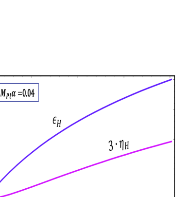
Figure 1: Dependence of $\epsilon_{H},3\eta_{H}$ and $\xi_{H}$ on the value of $\epsilon$, for $M_{Pl}\alpha=0.04$.

Since, within our model, via Eq. (2) VSR parameters are related to each other as

$$\eta=\epsilon-\frac{1}{2}(M_{Pl}\alpha)^{2}~{},~{}~{}~{}~{}\xi=-2(M_{Pl}\alpha)^{2}\epsilon,$$ (14)

the three equation in (6) can be rewritten as

$$\epsilon_{H}\left(\frac{3-\eta_{H}}{3-\epsilon_{H}}\right)^{2} = \epsilon$$

$$\frac{3(\epsilon_{H}+\eta_{H})-\eta_{H}^{2}-\xi_{H}}{3-\epsilon_{H}} = \epsilon-\frac{1}{2}(M_{Pl}\alpha)^{2}$$

$$3\frac{3-\eta_{H}}{(3-\epsilon_{H})^{2}}\left(3\epsilon_{H}\eta_{H}+\xi_{H}(1-\eta_{H})\right) = -2(M_{Pl}\alpha)^{2}\epsilon~{},$$ (15)

where $\sigma_{H}$ has been dropped because of it’s smallness. From the system of (15), for a fixed value of $M_{Pl}\alpha$, the parameters $\epsilon_{H},\eta_{H}$ and $\xi_{H}$ can be found in terms of the single parameter $\epsilon$. The dependance of these parameters on the value of $\epsilon$, for $M_{Pl}\alpha=0.04$ are shown in Fig. 1 (for different values of $M_{Pl}\alpha$ shapes of the curves are similar). We see that $\epsilon_{H}=1$ is achieved when $\epsilon=\epsilon_{e}\approx 2$ and thus, the expansion with respect to $\epsilon,\eta$ within this stage of inflation is invalid. On the other hand, the values of $\eta_{H}$ and $\xi_{H}$ remain relatively small. From the relation $2\epsilon=(M_{Pl}\alpha)^{2}\tan^{2}\frac{\alpha\phi_{\Theta}}{2}$ one derives:

$$d\phi_{\Theta}=\frac{M_{Pl}\sqrt{2}}{\sqrt{\epsilon}(2\epsilon+(M_{Pl}\alpha)^{2})}d\epsilon.$$ (16)

Using this, the integral in (3) can be rewritten as

$$N_{e}^{\rm inf}=\int_{\epsilon_{e}}^{\epsilon_{i}}\!\!\!\frac{1}{2\epsilon+(M_{Pl}\alpha)^{2}}\frac{d\epsilon}{\sqrt{\epsilon\epsilon_{H}}}~{}.$$ (17)

Having the numerical dependence $\epsilon_{H}=\epsilon_{H}(\epsilon)$ (depicted in Fig. 1), we can evaluate the integral in (17) and find $N_{e}^{\rm inf}$ for various values of $M_{Pl}\alpha$. The results are given in Fig. 2. While BICEP2/Keck and Planck [13] reported the bound $r\stackrel{{\scriptstyle<}}{{{}_{\sim}}}0.12$, upon generating the curves of Fig. 2 we also allowed larger values of $r$. Curves in Fig. 2 and also Table 1 demonstrate that, within natural inflation, with values $n_{s}\stackrel{{\scriptstyle<}}{{{}_{\sim}}}0.962$ (the previous Planck 2013 value) and $r\stackrel{{\scriptstyle>}}{{{}_{\sim}}}0.1$ or $n_{s}\stackrel{{\scriptstyle<}}{{{}_{\sim}}}0.953$ and $r\stackrel{{\scriptstyle>}}{{{}_{\sim}}}0.05$ there is an upper bound on $N_{e}^{\rm inf}$:

$$N_{e}^{\rm inf}\stackrel{{\scriptstyle<}}{{{}_{\sim}}}55.$$ (18)

Turned around this also implies that violating the bound (18), say $N_{e}^{\rm inf}\sim 60$, indicates larger $n_{s}$ and/or smaller $r$. Present Planck 2015 data seems to favor this. Bound (18) (if realized) would lead to another striking prediction and constraint.

Figure 2: Number of e-foldings. Solid lines correspond to the values of $n_{s}$ which fit with the current experimental data within $2\sigma$ error bars (with no restriction on $r$). Shaded areas correspond to the marginalized joint $68\%$ CL regions, given recently in [4] for $(n_{s},r)$ pairs, mapped by us to the $(M_{Pl}\alpha,N_{e}^{\rm inf})$ pairs for natural inflation. Gray background corresponds to the Planck TT$+$lowP, while red and blue colors represent Planck TT$+$LowP$+$BKP and Planck TT$+$LowP$+$BKP$+$BAO respectively (see Ref. [4] for an explanation of these combinations).

As discussed in Refs. [28], [5], the $N_{e}^{\rm eff}$, guaranteeing causality of fluctuations, should satisfy:

$$N_{e}^{\rm inf}=62-\ln\frac{k}{a_{0}H_{0}}-\ln\frac{10^{16}{\rm GeV}}{{\cal V}_{i}^{1/4}}+\ln\frac{{\cal V}_{i}^{1/4}}{{\cal V}_{e}^{1/4}}-\frac{4-3\gamma}{3\gamma}\ln\frac{{\cal V}_{e}^{1/4}}{\rho_{reh}^{1/4}}~{},$$ (19)

where for the scale $k$ we take $k=0.002\hskip 1.70717pt{\rm Mpc}^{-1}$, while the present horizon scale is $a_{0}H_{0}\approx 0.00033\hskip 1.70717pt{\rm Mpc}^{-1}$. The factor $\gamma$ accounts for the dynamics of the inflaton’s oscillations [29], [30] after inflation, and can be for our model approximated as $\gamma\simeq 1-\frac{1}{16}\frac{{\cal V}_{e}}{{\cal V}_{0}}$ (will turn out to be a pretty good approximation).

To reconcile the first two entries ($62-\ln\frac{k}{a_{0}H_{0}}\approx 60.2$) of Eq. (19) with the bound of Eq. (18) (see also Fig. 2), the remaining entries of Eq. (19) should be significant enough to bring $N_{e}^{\rm inf}$ down (at least) to $\approx 55$. The $3^{\rm rd}$ and $4^{\rm th}$ entries on the r.h.s. of Eq. (19) can be calculated with help of another observable - the amplitude of curvature perturbation $A_{s}$, which according to the Planck measurements [4], [5], should satisfy $A_{s}^{1/2}=4.686\times 10^{-5}$ (this value corresponds to the $\Lambda$CDM model). Generated by inflation, this parameter is given by:

$$A_{s}^{1/2}=\frac{1}{\sqrt{12}\pi}\left|\frac{{\cal V}^{3/2}}{M_{Pl}^{3}{\cal V}^{\prime}}\right|_{\phi_{\Theta}^{i}}\simeq\frac{4\sqrt{6}}{3\pi}\frac{{\cal V}_{0}^{1/2}}{M_{Pl}^{2}}\frac{M_{Pl}\alpha}{r(1+8(M_{Pl}\alpha)^{2}/r)^{1/2}}~{}.$$ (20)

$$\begin{array}[]{|c|c|c|c|c|c|c|c|c|}\hline\cr\vspace{-0.4cm}\hfil&&&&&&&&\\ \vspace{-0.4cm}\par r&M_{Pl}\alpha&\hskip 0.85358ptn_{s}&10^{4}\!\times\!\frac{dn_{s}}{d\ln k}&\hskip 0.85358ptN_{e}^{\rm inf}&\hskip 1.42262pt\frac{{\cal V}_{0}^{1/4}}{10^{16}{\rm GeV}}&\hskip 1.42262pt\frac{{\cal V}_{i}^{1/4}}{10^{16}{\rm GeV}}&\hskip 1.42262pt\frac{{\cal V}_{e}^{1/4}}{10^{16}{\rm GeV}}&\rho_{reh}^{1/4}({\rm GeV})\\ &&&&&&&&\\ \hline\cr\hline\cr&0.001&0.962&-7.1&53.62&19.8&2.01&0.53&3.14\!\cdot\!\!10^{4}\\ \vspace{-0.2cm}\hfil&0.04&0.961&-7.71&51.47&3.2&2.01&0.54&53.7\\ \vspace{-0.3cm}0.15&&&&&&&&\\ &0.055&0.959&-8.25&49.73&2.77&2.01&0.54&0.31\\ &0.065&0.958&-8.71&48.39&2.58&2.01&0.55&0.006\\ \hline\cr\hline\cr&0.04&0.967&-5.43&61.25&2.92&1.92&0.49&2.77\!\cdot\!\!10^{14}\\ &0.06&0.965&-6.06&57.92&2.45&1.92&0.5&1.39\!\cdot\!\!10^{10}\\ 0.125&0.08&0.962&-6.95&53.96&2.2&1.92&0.52&1.14\!\cdot\!\!10^{5}\\ &0.1&0.959&-8.09&49.79&2.04&1.92&0.54&0.5\\ &0.11&0.957&-8.76&47.72&2&1.92&0.55&0.001\\ \hline\cr\hline\cr&0.097&0.966&-5.53&60&1.89&1.81&0.49&9.2\!\cdot\!\!10^{12}\\ &0.1&0.965&-5.68&59.14&1.87&1.81&0.5&7.13\!\cdot\!\!10^{11}\\ 0.1&0.12&0.961&-6.79&53.58&1.79&1.82&0.52&5\!\cdot\!\!10^{4}\\ &0.135&0.957&-7.77&49.7&1.74&1.82&0.54&0.52\\ &0.143&0.955&-8.33&47.76&1.72&1.82&0.55&0.0017\\ \hline\cr\hline\cr&0.172&0.958&-4.53&59.5&1.35&1.53&0.47&4.8\!\cdot\!\!10^{12}\\ &0.19&0.952&-5.36&53.48&1.34&1.53&0.49&8.7\!\cdot\!\!10^{4}\\ \vspace{-0.3cm}\hfil&0.194&0.95&-5.55&50.93&1.34&1.53&0.49&44.8\\ \vspace{-0.3cm}0.05&&&&&&&&\\ &0.2&0.948&-5.86&50.51&1.33&1.53&0.5&13.6\\ &0.205&0.946&-6.12&49.12&1.33&1.53&0.5&0.225\\ &0.21&0.944&-6.39&47.78&1.33&1.53&0.51&0.0044\\ \hline\cr\end{array}$$

Table 1: Numerical Results for different values of $r$ and $M_{Pl}\alpha$. For all cases $A_{s}^{1/2}=4.686\times 10^{-5}.$

In order to obtain the observed value of $A_{s}^{1/2}$, for typical $r=0.12$ and $M_{Pl}\alpha\sim 0.1$ we need to have ${\cal V}_{0}^{1/4}\sim 10^{-2}M_{Pl}$. This, on the other hand, gives ${\cal V}^{1/4}_{i}\sim 0.01M_{Pl}$ and ${\cal V}_{e}^{1/4}\sim 2\cdot 10^{-3}M_{Pl}$. Using these values in (19) we see that the sum of the $3^{\rm rd}$ and $4^{\rm th}$ terms is$\approx 3.4$. Thus, the last term should be responsible for a proper reduction of $N_{e}^{\rm inf}$. Namely, during the reheating process, the universe should expand by nearly $10$ (or even more) e-foldings. This means that, for this case, the model should have a significant reheat history with $\rho_{reh}^{1/4}\sim 100$ GeV. Within the scenario of natural inflation, this has not been appreciated before. For lower $r$ and appropriate values of $M_{Pl}\alpha$ (and $n_{s}$) the reheating temperature can be big. The concise numerical results (compared to the rough evaluation below Eq. (20)) are given in Table 1, where we considered cases with $\rho_{reh}^{1/4}$ not smaller than $10^{-3}$ GeV, and $N_{e}^{\rm inf}\leq 62$. The values of the spectral index running $\frac{dn_{s}}{d\ln k}=16\epsilon_{i}\eta_{i}-24\epsilon_{i}^{2}-2\xi_{i}$ are also presented. The first three row-blocks correspond to the values of $n_{s}$ within $2\sigma$ ranges of the current experimental data. The first three cases of the bottom block correspond to the $n_{s}$ within $3\sigma$ range, while the last three lines of this block have lower values of $n_{s}$ (beyond the $3\sigma$ deviation). Since the issue for the value of $r$ is not fully settled yet, we have included moderately large values of $r$($\leq 0.15$). At the bottom block of the table we gave results for $r=0.05$, which corresponds to the peak of the $r$’s likelihood curve presented by the joint analysis of BICEP2/Keck and Planck [13]. Note that the results presented here are consistent with the analysis for natural inflation carried out before [8] (see $2^{\rm nd}$ citation of this Ref.).

Below we will show that within our scenario of natural inflation, a low reheat temperature is realized naturally.

3 Natural inflation from 5D SUGRA

In order to address the details of inflaton decay, related to the reheat temperature, we need to specify the underlying theory natural inflation emerged from. A very good candidate is a higher dimensional construction [6]. Here we present a 5D conformal SUGRA realization [1] of this idea, using the off-shell superfield formulation developed in Refs. [19], [20].

Lagrangian couplings, for the bulk ${\bf H}=(H,~{}H^{c})$ hypermultiplets’, components are:

$$e_{(4)}^{-1}{\cal L}(H)=\int d^{4}\theta(T+T^{\dagger})\left(H^{\dagger}H+H^{c\dagger}H^{c}\right)+\int d^{2}\theta\left(2H^{c}\partial_{y}H+g_{1}\Sigma_{1}(e^{{\rm i}\hat{\theta}_{1}}H^{2}-e^{-{\rm i}\hat{\theta}_{1}}H^{c2})\right)+{\rm h.c.}$$ (21)

where the odd fields $V_{i}$ are set to zero. $\Sigma_{1}$ is the $Z_{2}$ even $5^{\rm th}$ component of the 5D $U(1)$ vector supermultiplet. With the parity assignments

$$Z_{2}:~{}~{}~{}H\to H~{},~{}~{}~{}~{}~{}H^{c}\to-H^{c}~{},$$ (22)

the KK decomposition for $H$ and $H^{c}$ superfields is given by

$$H=\frac{1}{2\sqrt{\pi R}}H^{(0)}+\frac{1}{\sqrt{2\pi R}}\sum_{n=1}^{+\infty}H^{(n)}\cos\frac{ny}{R}~{},~{}~{}~{}~{}~{}H^{c}=\frac{1}{\sqrt{2\pi R}}\sum_{n=1}^{+\infty}\overline{H}^{\hskip 1.70717pt(n)}\sin\frac{ny}{R}~{}.$$ (23)

With these decompositions, and steps given in Appendix A, we can calculate the mass spectrum of KK states, their couplings to the inflaton and with these, the one loop order inflation potential (dropping higher winding modes) having the form of (1) with

$$\alpha=\pi g_{4}R,~{}~{}~{}~{}~{}~{}{\cal V}_{0}=\frac{3}{16\pi^{6}R^{4}}{\cal B}~{}~{}~{}{\rm and}~{}~{}~{}{\cal B}=1-\cos(\pi R|F_{T}|)~{}.$$ (24)

The 4D inflaton field $\phi_{\Theta}$ is related to the 5D $U(1)$ gauge field $A_{5}^{1}$ as:

$$\phi_{\Theta}=\sqrt{2\pi R}A_{5}^{1}~{}.$$ (25)

Since the model is well defined, we also can write down the inflaton coupling with the components of $H$. The latter, having a coupling with the SM fields, would insure the inflaton decay and the reheating of the Universe. In our setup, we assume that all MSSM matter and scalar superfields are introduced at the $y=0$ brane. Since $H$ is even under orbifold parity and a singlet under all SM gauge symmetries, it can couple to the MSSM states through the following brane superpotential couplings

$${\cal L}_{H-br}=\sqrt{2\pi R}\int d^{2}\theta dy\delta(y)\lambda lh_{u}H+{\rm h.c.}$$ (26)

where $l$ and $h_{u}$ are 4D $N=1$ SUSY superfields corresponding to lepton doublets and up type higgs doublet superfields respectively. In Eq. (26), without loss of generality, only one lepton doublet (out of three lepton families) is taken to couple with the $H$,

$${\cal L}_{H-br}\supset-\lambda\!\!\left((\frac{1}{\sqrt{2}}\psi_{H}^{(0)}+\sum_{n=1}^{+\infty}\psi_{H}^{(n)})(lh_{u}+\tilde{l}\tilde{h}_{u})+(\frac{1}{\sqrt{2}}H^{(0)}+\sum_{n=1}^{+\infty}H^{(n)})l\tilde{h}_{u}\right.$$

$$-\left.(\frac{1}{\sqrt{2}}F_{H}^{(0)}+\sum_{n=1}^{+\infty}F_{H}^{(n)})\tilde{l}h_{u}\right)+{\rm h.c.}$$ (27)

where $l$ now denotes the fermionic lepton doublet and $h_{u}$ an up-type higgs doublet. States $\tilde{l}$ and $\tilde{h}_{u}$ stand for their superpartners respectively. $H^{(n)}$ and $\psi_{H}^{(n)}$ in Eq. (27) indicate scalar and fermionic components of the superfield $H$.

Upon eliminating all $F$-terms and heavy fermionic and scalar states (in the $H$ and $H^{c}$ superfields), we can derive effective operators containing the inflaton linearly. As it will turn out within the model considered (see discussion in Appendix A.1), the $\tilde{l}$ states are heavier than the inflaton and operators containing $\tilde{l}$ are irrelevant for the inflaton decay. Thus, the effective operators, needed to be considered, are

$$\phi_{\Theta}\left(C_{0}(lh_{u})^{2}+C_{1}(l\tilde{h}_{u})^{2}+{\rm h.c.}\right)+C_{2}\phi_{\Theta}(l\tilde{h}_{u})(\bar{l}\bar{\tilde{h}}_{u}).$$ (28)

These terms should be responsible for the inflaton decay. Derivation and form of the $C$-coefficients are given in Appendix A.

3.1 Inflaton Decay and Reheating

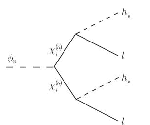
Figure 3: Diagram responsible for the inflaton’s dominant decay.

As was mentioned above and shown in Appendix A.1, the slepton states $\tilde{l}$ have masses $\frac{1}{2}|F_{T}|\sim 1/(2R)$ and thus are heavier than the inflaton. Indeed, the latter’s mass, obtained from the potential, is:

$$M_{\phi_{\Theta}}=\frac{g_{4}\sqrt{3}(1-\cos(\pi R|F_{T}|))^{1/2}}{4\pi^{2}R}\ll\frac{1}{R}~{}.$$ (29)

($g_{4}\ll 1$ for successful inflation). Thus the inflaton decay in channels containing $\tilde{l}$ is kinematically forbidden. Anticipating, we note that the preheating process by inflaton decay in heavy states is excluded within our scenario with parameters we consider (this is shown at the end of this subsection). Thus, the reheating proceeds by perturbative 4-body decay of the inflaton.

Among operators generated via exchange of heavy fermionic $\chi_{i}^{(n)}$ and scalar $S_{i}^{(n)}$ states, only those given in Eq. (28) are relevant. For calculating the decay widths (in a pretty good approximation) it is enough to have the form of the $C_{i}$ coefficients.

As shown in Appendix A, within our model $C_{2}=0$ and the corresponding operator does not play any role. Moreover, according to Eqs. (A.26) and (A.30) we have $C_{0}\sim R^{2}$ (due to a $1/m_{\psi_{H}}^{2}$) and $C_{1}\sim R^{3}$ (with $|F_{T}|\sim 1/R$, dictated from the inflation). Thus, we get an estimate for the following branching ratio

$$\frac{\Gamma(\phi_{\Theta}\to ll\tilde{h}_{u}\tilde{h}_{u})}{\Gamma(\phi_{\Theta}\to llh_{u}h_{u})}\sim\frac{|C_{1}|^{2}M_{\phi_{\Theta}}^{7}}{|C_{0}|^{2}M_{\phi_{\Theta}}^{5}}\sim(RM_{\phi_{\Theta}})^{2}\sim\frac{3g_{4}^{2}}{16\pi^{4}}\ll 1~{}.$$ (30)

This means that the inflaton decay is mainly due to the $C_{0}$ operator [see Eqs. (28 and (A.26), with gauge coupling $g_{4}$ and Yukawa coupling $\lambda$], i.e. in the channel $\phi_{\Theta}\to llh_{u}h_{u}$ (the diagram in Fig. 3. Remember: $l$ denotes the SM lepton doublet and $h_{u}$ the scalar up type higgs doublet). For simplicity we assume that the state $h_{u}$ includes the light SM higgs doublet $h$ with weight nearly equal to one, i.e. $h_{u}\stackrel{{\scriptstyle\supset}}{{{}_{\sim}}}h$.

For the decay width we get:

$$\Gamma(\phi_{\Theta})\simeq\Gamma(\phi_{\Theta}\to llh_{u}h_{u})=\frac{9}{9\cdot 2^{7}(2\pi)^{5}}|C_{0}|^{2}M_{\phi_{\Theta}}^{5}~{}.$$ (31)

The factor $9$ in the numerator accounts for the multiplicity of final states. (The final $llh_{u}h_{u}$ channel includes three combinations $e^{-}e^{-}h^{+}h^{+}$, $\nu\nu h^{0}h^{0}$, $e^{-}\nu h^{+}h^{0}$ and for each pair of identical final states a factor $2$ should be included.) The denominator factors in (31) come from the phase space integration. Using the form of $C_{0}$, given by Eq. (A.26), in expression (31), we get:

$$\Gamma(\phi_{\Theta})\simeq\frac{g_{4}^{2}|\lambda|^{4}}{2^{18}\pi}(RM_{\phi_{\Theta}})^{4}M_{\phi_{\Theta}}~{}.$$ (32)

Expressing $\rho_{reh}=\frac{\pi^{2}}{30}g_{*}T_{r}^{4}$ through the reheat temperature [33]

$$T_{r}=\left(\frac{90}{\pi^{2}g_{*}}\right)^{1/4}\!\!\sqrt{M_{Pl}\Gamma(\phi_{\Theta})}$$ (33)

($g_{*}$ is the number of relativistic degrees at temperature $T_{r}$) and using expressions (32) and (29), we get

$$\rho_{reh}^{1/4}=1.316\left(M_{Pl}\Gamma(\phi_{\Theta})\right)^{1/2}=5.85\cdot 10^{-7}M_{Pl}\frac{g_{4}^{7/2}|\lambda|^{2}}{(RM_{Pl})^{1/2}}(1-\cos(\pi R|F_{T}|))^{5/4}.$$ (34)

From this, with $RM_{Pl}\sim 10$, $R|F_{T}|\sim 1$ and $g_{4}\sim 1.5\cdot 10^{-3}$ we obtain $\rho_{reh}^{1/4}\sim|\lambda|^{2}\times 100$ GeV.

$$\begin{array}[]{|c|c|c|c|c|c|c|}\hline\cr\vspace{-0.4cm}\hfil&&&&&&\\ \vspace{-0.4cm}\par(r,~{}n_{s})&M_{Pl}\alpha&\hskip 1.42262pt\frac{{\cal V}_{0}^{1/4}}{10^{16}{\rm GeV}}&\hskip 0.85358ptR|F_{T}|&\hskip 0.85358ptRM_{Pl}&\hskip 1.42262ptg_{4}&\hskip 1.42262pt\frac{\rho_{reh}^{1/4}}{|\lambda|^{2}}({\rm GeV})\\ &&&&&&\\ \hline\cr\hline\cr\vspace{-0.3cm}\hfil&&&0.75&10.1&1.26\!\cdot\!10^{-3}&60.5\\ \vspace{-0.3cm}(0.15,0.961)&0.04&3.2&&&&\\ &&&0.9&10.5&1.22\!\cdot\!10^{-3}&62.6\\ \hline\cr\hline\cr\vspace{-0.3cm}\hfil&&&0.5&10.2&1.71\!\cdot\!10^{-3}&90.6\\ \vspace{-0.3cm}(0.15,0.959)&0.055&2.77&&&&\\ &&&0.9&12.1&1.45\!\cdot\!10^{-3}&107\\ \hline\cr\hline\cr\vspace{-0.3cm}\hfil&&&0.5&11&1.88\!\cdot\!10^{-3}&122\\ \vspace{-0.3cm}(0.15,0.958)&0.065&2.58&&&&\\ &&&0.9&13&1.6\!\cdot\!10^{-3}&145\\ \hline\cr\hline\cr\vspace{-0.3cm}\hfil&&&0.5&13.9&2.29\!\cdot\!10^{-3}&216\\ \vspace{-0.3cm}(0.125,0.959)&0.1&2.04&&&&\\ &&&0.9&16.4&1.94\!\cdot\!10^{-3}&255\\ \hline\cr\hline\cr\vspace{-0.3cm}\hfil&&&0.5&16.3&2.64\!\cdot\!10^{-3}&327\\ \vspace{-0.3cm}(0.1,~{}0.957)&0.135&1.74&&&&\\ &&&0.9&19.3&2.23\!\cdot\!10^{-3}&386\\ \hline\cr\hline\cr\vspace{-0.3cm}\hfil&&&0.5&21&2.91\!\cdot\!10^{-3}&409\\ \vspace{-0.3cm}(0.05,~{}0.95)&0.194&1.34&&&&\\ &&&0.9&25&2.45\!\cdot\!10^{-3}&483\\ \hline\cr\hline\cr\vspace{-0.3cm}\hfil&&&0.5&21.3&3\!\cdot\!10^{-3}&442\\ \vspace{-0.3cm}(0.05,0.948)&0.2&1.33&&&&\\ &&&0.9&25.2&2.53\!\cdot\!10^{-3}&522\\ \hline\cr\hline\cr\vspace{-0.3cm}\hfil&&&0.2&14.1&4.74\!\cdot\!10^{-3}&346\\ \vspace{-0.3cm}(0.05,0.944)&0.21&1.33&&&&\\ &&&0.9&25.2&2.65\!\cdot\!10^{-3}&619\\ \hline\cr\end{array}$$

Table 2: Values of $RM_{Pl}$, $g_{4}$ and $\rho_{reh}^{1/4}$ for different cases of successfull inflation.

Our 5D SUGRA construction allows more accurate estimates, because some of the parameters are related to each other. For instance, from (24) we have

$$R\simeq\frac{0.118}{{\cal V}_{0}^{1/4}}(1-\cos(\pi R|F_{T}|))^{1/4}~{},$$ (35)

$$g_{4}=\frac{\alpha}{\pi R}~{}.$$ (36)

From (35) we see that in order to have $RM_{Pl}\stackrel{{\scriptstyle>}}{{{}_{\sim}}}10$ we need ${\cal V}_{0}^{1/4}\stackrel{{\scriptstyle<}}{{{}_{\sim}}}3.4\cdot 10^{16}$ GeV. The latter value suites well with most of the values of ${\cal V}_{0}^{1/4}$ given in Table 1 (calculated from the inflation potential). At the same time, we see from (35) that $|F_{T}|$ can not be suppressed and should be $|F_{T}|\sim 1/R$. Using Eqs. (35) and (36) in (34), we obtain

$$\rho_{reh}^{1/4}=5.45\cdot 10^{-5}M_{Pl}(\alpha M_{Pl})^{7/2}\left(\frac{{\cal V}_{0}^{1/4}}{M_{Pl}}\right)^{\!\!4}|\lambda|^{2}(1-\cos(\pi R|F_{T}|))^{1/4}.$$ (37)

This expression is useful to find the maximal value of $\rho_{reh}^{1/4}$. Using the pairs of $(\alpha M_{Pl},{\cal V}_{0})$ given in Table 1, from Eq. (37) it turns out that $\rho_{reh}^{1/4}\stackrel{{\scriptstyle<}}{{{}_{\sim}}}|\lambda|^{2}\times 619$ GeV. This is an upper bound on the reheating energy density obtained within our 5D SUGRA scenario. In Table 2 we give the values of $RM_{Pl}$, $g_{4}$ and $\rho_{reh}^{1/4}$ for various cases. Input values of ${\cal V}_{0}^{1/4}$ and $M_{Pl}\alpha$ were taken from Table 1, which correspond to successful inflation. Also, we have selected the values of $R|F_{T}|$ in such a way as to get $RM_{Pl}\stackrel{{\scriptstyle>}}{{{}_{\sim}}}10$. We see that within $2\sigma$ deviations of $n_{s}$ we have $\rho_{reh}^{1/4}\stackrel{{\scriptstyle<}}{{{}_{\sim}}}|\lambda|^{2}\times 386$ GeV, corresponding to reheat temperatures $T_{r}\stackrel{{\scriptstyle<}}{{{}_{\sim}}}|\lambda|^{2}\times 130$ GeV. These values can be easily reconciled with those low values of $\rho_{reh}^{1/4}$, given in Table 1, by natural selection of the brane Yukawa coupling $\lambda$ in a range $1/300\stackrel{{\scriptstyle<}}{{{}_{\sim}}}\lambda\stackrel{{\scriptstyle<}}{{{}_{\sim}}}1$.

Excluding Preheating

Since in the presented 5D SUGRA scenario the inflaton has direct couplings with heavy KK states of $H$ and $H^{c}$ superfields, we need to make sure that after inflation, during the inflaton oscillation there is no production of these heavy states and no reheat is anticipated by the preheating process. Below we show that indeed, within our model preheating does not take place.

Starting from the fermionic KK states (which turned out to dominate in reheating), their masses are given by Eq. (A.16). with $\langle M^{1}\rangle=0$ and shift of the inflaton around the vacuum

$$g_{1}A_{5}^{1}=g_{1}\langle A_{5}^{1}\rangle+g_{1}\hat{A}_{5}^{1}=\frac{1}{R}+g_{4}\hat{\phi}_{\Theta}~{}$$ (38)

for fermion masses we get

$$m_{\chi_{1}}^{(n)}=\frac{1}{2}\left|\frac{2n+1}{R}+g_{4}\hat{\phi}_{\Theta}\right|~{},~{}~{}~{}~{}m_{\chi_{2}}^{(n)}=\frac{1}{2}\left|\frac{2n-1}{R}-g_{4}\hat{\phi}_{\Theta}\right|~{}.$$ (39)

The $\hat{\phi}_{\Theta}$ is the quantum part oscillating around the potential’s minimum (after the end of inflation) and finally relaxing to $\hat{\phi}_{\Theta}=0$. Our aim is to see if either of the masses in (39) become zero during inflaton damped oscillation. As was shown in Ref. [34], this is the criterion for the fermionic preheating.

The amplitude of $\hat{\phi}_{\Theta}$ has a well defined value at the end of the inflation when slow roll breaks down, i.e. at the point $\epsilon=\epsilon_{f}\simeq 2$. With $\epsilon=\frac{1}{2}(M_{Pl}\alpha)^{2}\cot^{2}(\pi Rg_{4}\hat{\phi}_{\Theta}/2)$, for times $t>t_{f}$ we have

$$|g_{4}\hat{\phi}_{\Theta}^{f}|=\frac{1}{R}\frac{2}{\pi}{\rm ArcTan}\left(\frac{M_{Pl}\alpha}{\sqrt{2\epsilon_{f}}}\right)\simeq\frac{1}{R}\frac{M_{Pl}\alpha}{\pi}~{}.$$ (40)

On the other hand, from our Table 2 we have $M_{Pl}\alpha\stackrel{{\scriptstyle<}}{{{}_{\sim}}}0.2$. Using this in (40), we get

$$|g_{4}\hat{\phi}_{\Theta}^{f}|\stackrel{{\scriptstyle<}}{{{}_{\sim}}}\frac{0.064}{R}.$$ (41)

The kinetic energy of the oscillation is still at most comparable at the end of inflation and there is also damping. Thus, Eq. (41) is a good estimate for the maximal amplitude of $\hat{\phi}_{\Theta}$. With this bound, we can see that the term $g_{4}\hat{\phi}_{\Theta}$ in Eq. (39) will not be able to nullify fermion masses during inflaton oscillations. This fact, as was shown in Ref. [34], prevents KK fermion production and no fermionic preheating takes place.

Now we turn to the scalar KK states. With Eqs. (A.10), (38) and $\langle M^{1}\rangle=0$ for the scalar masses we get

$$(m_{1,2}^{(n)})^{2}\!=\frac{1}{4}\!\left(\frac{2n+1}{R}\pm|F_{T}|+g_{4}\hat{\phi}_{\Theta}\right)^{2},~{}~{}~{}~{}~{}~{}(m_{3,4}^{(n)})^{2}\!=\frac{1}{4}\!\left(\frac{2n-1}{R}\mp|F_{T}|-g_{4}\hat{\phi}_{\Theta}\right)^{2}~{}.$$ (42)

Therefore, with Eq. (41) and the values of $|F_{T}|$ given in Table 2, we see that masses in (42) never cross zero and for the positively defined mass² of the $S_{i}$ states we have

$$(m_{i}^{(n)})^{2}\stackrel{{\scriptstyle>}}{{{}_{\sim}}}\left(\frac{0.036}{R}\right)^{2}\gg 10^{4}\times(M_{\phi_{\Theta}})^{2}~{},$$ (43)

where the inflaton mass $M_{\phi_{\Theta}}\sim 10^{13}$ GeV. Therefore, all modes from the scalar KK tower are much heavier (by a factor $>100$) than the inflaton mass for any time during the inflaton’s oscillation. As was shown in Refs. [33], [35] for these conditions the amplification and/or production of the scalar modes never happens. This excludes preheating also via the scalar production. Within our scenario this result is insured by the gauge symmetry, because the inflaton in the heavy KK states’ masses contributes in the combination $g_{4}\hat{\phi}_{\Theta}$ [see e.g. Eqs. (39) and (42)].

Thus, we finally conclude that within our scenario reheating occurs by the perturbative inflaton four-body decays discussed at the beginning of Sec. 3.1

4 Discussion and Concluding Remarks

In the effective action of our 5D conformal SUGRA model the $5$-th component ($\Sigma_{1}$) of a $U(1)$ vector supermultiplet couples to a charged hypermultiplet $(H,H^{c})$. This, due to a fixed compactification radius $R$ leads to the potential of natural inflation for the CP odd part of $\Sigma_{1}$, neglecting the suppressed higher winding modes. We analysed this potential like in [8] putting emphasis on the potential of inflation and the number of e-folds of perturbations leaving the horizon. This we compared with the number of e-folds required by a causal connection between the observed universe background fluctuations and by the size of observed curvature perturbations. For a large tensor component $r\stackrel{{\scriptstyle>}}{{{}_{\sim}}}0.1$ and $n_{s}\stackrel{{\scriptstyle<}}{{{}_{\sim}}}0.962$ or $r\stackrel{{\scriptstyle>}}{{{}_{\sim}}}0.05$ and $n_{s}\stackrel{{\scriptstyle<}}{{{}_{\sim}}}0.953$ close to the lower bound of present Planck 2015 data a small $N_{e}^{\rm inf}\stackrel{{\scriptstyle<}}{{{}_{\sim}}}55$ results. This requires a small reheating temperature. We inspected the decay of the gauge inflaton to the light MSSM fields living on a brane. These decays are mediated by the bulk hypermultiplet $H$. The very same $H$ hypermultiplet, together with it’s $SU(2)_{R}$ partner $H^{c}$, generates the inflation potential. The $H$ is assumed to have superpotential Yukawa couplings to brane fields with a Yukawa strength $\lambda\stackrel{{\scriptstyle<}}{{{}_{\sim}}}1$. Due to a very small gauge coupling and to a relatively light inflaton this led to a suppressed decay width and reheat temperature $T_{r}\sim|\lambda|^{2}\times 100$ GeV. Within the considered scenario the dominant 4-body decays of the inflaton are mediated by fermionic components $\psi_{H}$ (of $H$) with $llhh$ final states (two lepton and two higgs doublets’ components). Other channels are either kinematically forbidden due to heavy sleptons $\tilde{l}$ gaining large masses through the large $F_{T}$ term, a case of split SUSY, or are suppressed (due to the small inflaton mass $M_{\phi_{\Theta}}\ll 1/R$) by an additional small factor $(RM_{\phi_{\Theta}})^{2}$. Therefore, a similar mechanism can be realized also for extranatural inflation [6] without supersymmetry with a bulk fermionic $\psi_{H}$ generating the inflation potential and brane Yukawa coupling $\lambda lh\psi_{H}$. Within our model (as shown in Appendix A), due to specific bulk couplings and degeneracy, the lepton number is conserved and neutrinos stay massless (and this remains true for extra natural inflation). The situation can be changed by introducing a brane Majorana mass term $\frac{1}{2}M_{br}HH$ and it is inviting to exploit such a possibility. Since this is not directly related to inflation, on one side, and trying to keep the calculus simple on the other side, we have not pursued this possibility in this paper and reserved it for future studies.

The model of [1], reanalyzed here in more detail, is by no means complete. A concrete mechanism for radion stabilization like in Ref. [24] has to be presented and the breaking of 4D SUSY has to be worked out in more detail. Here and in [1] we concentrated on the aspects that our model originates in a very straightforward way from 5D conformal SUGRA -which can be also interpreted as a result of M-theory [20] - and that the inflaton is related to a gauge field. If the new BICEP2 data, advertising large tensorial fluctuations, will turn out not to be mainly dust effects and if in the future, the value of $r$ turns out to be unsuppressed (i.e. $r\stackrel{{\scriptstyle>}}{{{}_{\sim}}}0.05$ or so) and if $n_{s}$ will not remain very close to the presently favored higher values, then some form of natural inflation derived from 5D gauge inflation would be indeed a suitable and attractive candidate for inflationary model building. If further findings will indicate a really small value of $r$, then as an alternative, the ’modulus’ inflation of[1] should be pursued. This would mean that the inflaton is the real part of the $\Sigma_{1}$ chiral supermultiplet scalar component. Also, a more general two field inflation [10] from complex $\Sigma_{1}$ could get into focus again.

Acknowledgments

We thank Arthur Hebecker and Valeria Pettorino for discussions. Research of Z.T. is partially supported by Shota Rustaveli National Science Foundation (Contracts No. 31/89 and No. DI/12/6-200/13).

Appendix A KK spectrum and the inflaton effective couplings

First let us discuss the emergence of the non zero $F_{T}$ term of the $T$ radion superfield. This can be easily understood by the effective 4D SUGRA description developed in [20]. The 4D supergravity action is given by [38]

$${\cal L}_{D}^{(4D)}+{\cal L}_{F}^{(4D)}~{}~{}~{}~{}~{}~{}~{}~{}{\rm with}$$

$${\cal L}_{D}^{(4D)}=-3\int\!\!\!d^{4}\theta\,e^{-{\cal K}/3}\phi^{+}\phi,~{}~{}~{}~{}~{}~{}~{}~{}~{}~{}~{}~{}~{}{\cal L}_{F}^{(4D)}=\int\!\!\!d^{2}\theta\phi^{3}\,W+\frac{1}{4}\int\!\!\!d^{2}\theta f_{IJ}{{\cal W}}^{\alpha I}{{\cal W}}_{\alpha}^{J}+{\rm h.c.}$$ (A.1)

where ${\cal K}$ and $W(\Phi)$ are the Kähler potential and the superpotential respectively, while $f_{IJ}(\Phi)$ is the gauge kinetic function. $\phi$ is the 4D compensator chiral superfield. Being a 4D effective theory, (A.1) would include zero modes of the 5D supermultiplets and the brane fields as well. Therefore, for the bulk states the form of (A.1) will be dictated by the $5D$ construction [20]. For instance, the 4D compensator $\phi$ is related with the 5D compensator as $\phi=\sqrt{2\pi R}\kappa_{5}^{-\frac{1}{3}}h^{\frac{2}{3}}$. From (A.1) we find the expressions for the F-terms:

$$F^{I}=-M_{P}e^{{\cal K}/3}{\cal K}^{I{\bar{J}}}D_{\bar{J}}{\bar{W}},~{}~{}~{}~{}F_{\phi}=M_{P}^{2}e^{{\cal K}/3}\left({\bar{W}}-\frac{1}{3}{\cal K}^{I{\bar{J}}}{\cal K}_{I}D_{\bar{J}}{\bar{W}}\right).$$ (A.2)

where $I$ runs over all scalars. By plugging Eq. (A.2) back in to (A.1), one derives the $F$-term scalar potential (by setting $\phi=M_{P}$ and going to the 4D Einstein-frame, rescaling the metric $g_{\mu\nu}\to e^{{\cal K}/3}g_{\mu\nu}$):

$$V_{F}=M_{P}^{4}\,e^{\cal K}\left({\cal K}^{I{\bar{J}}}D_{I}WD_{\bar{J}}{\bar{W}}-3|W|^{2}\right),~{}~{}~{}{\rm with}~{}~{}~{}D_{I}\equiv\partial_{I}+{\cal K}_{I}~{}.$$ (A.3)

For the $T$ modulus (the radion) the Kähler potential is ${\cal K}=-3\ln(T+T^{\dagger})$. For the time being we take $W=$const. for the superpotential. With these, it is easy to check that we get a flat potential $V_{F}=0$ with $F_{\phi}=0$ and $F_{T}=M_{P}W^{*}$. Thus, we have fixed a non zero $F_{T}$ which plays a crucial role for the generation of the inflaton potential. This is enough for performing a calculation of the KK spectrum and the 1-loop inflaton potential. We will come back to the SUSY breaking at the end, upon discussion of the superpartners’ spectrum from the MSSM brane fields.

Any bulk state transforming non trivially under $SU(2)_{R}$ feels $F_{T}$ SUSY breaking. This happens of course with the bulk hypers described by the terms in (21). With the parametrization

$$F_{T}=-|F_{T}|e^{i\alpha}~{},~{}~{}~{}~{}{\rm with}~{}~{}~{}~{}\alpha={\rm Arg}(F_{T})+\pi~{},$$ (A.4)

setting the scalar component of $T$ to one, and making a phase redefinition of the scalar components $H,H^{c}$:

$$H\to e^{-i(\hat{\theta}_{1}+\alpha)/2}H~{},~{}~{}~{}~{}~{}H^{c}\to e^{i(\hat{\theta}_{1}-\alpha)/2}H^{c}~{},$$ (A.5)

the couplings in (21) give the potential:

$$V(H)=2\left|\partial_{5}H-\frac{g_{1}}{2}(M^{1}-\frac{{\rm i}\Theta}{2\pi R})H^{c}-\frac{1}{2}|F_{T}|H^{c*}\right|^{2}+2\left|\partial_{5}H^{c}-\frac{g_{1}}{2}(M^{1}-\frac{{\rm i}\Theta}{2\pi R})H+\frac{1}{2}|F_{T}|H^{*}\right|^{2}+$$

$$\frac{1}{2}g_{1}M^{1}|F_{T}|(H^{2}-H^{c2})+\frac{1}{2}g_{1}M^{1}|F_{T}|(H^{*2}-H^{c*2})~{}.$$ (A.6)

With the decomposition of Eq. (23) and integrating along the fifth dimension $\int_{0}^{2\pi R}dy{\cal L}^{(5)}$ we obtain

$$V(H^{(n)})=\left|g_{1}\Sigma_{1}H^{(0)}-\frac{1}{2}|F_{T}|H^{(0)*}\right|^{2}+\sum_{n=1}^{+\infty}\left|\frac{n}{R}H^{(n)}\!+g_{1}\Sigma_{1}\overline{H}^{(n)}+\frac{1}{2}|F_{T}|\overline{H}^{(n)*}\right|^{2}+$$

$$\sum_{n=1}^{+\infty}\left|\frac{n}{R}\overline{H}^{(n)}\!-g_{1}\Sigma_{1}H^{(n)}+\frac{1}{2}|F_{T}|H^{(n)*}\right|^{2}\!+\frac{1}{4}g_{1}M^{1}|F_{T}|\left(\sum_{n=0}^{+\infty}(H^{(n)})^{2}-\sum_{n=1}^{+\infty}(\overline{H}^{(n)})^{2}+{\rm h.c.}\right)$$ (A.7)

$$H^{(0)}=\frac{1}{\sqrt{2}}(S^{(0)}_{1}+iS^{(0)}_{2})$$

$${\rm for}~{}~{}~{}n=1,\cdots,+\infty~{},~{}~{}~{}~{}~{}~{}\left(\!\!\begin{array}[]{c}{\rm Re}H^{(n)}\\ {\rm Im}H^{(n)}\\ {\rm Re}\overline{H}^{(n)}\\ {\rm Im}\overline{H}^{(n)}\\ \end{array}\!\!\right)\!\!=\!\frac{1}{2\sqrt{2}}\left(\!\begin{array}[]{cccc}1&1&\!\!\!-1&\!\!\!-1\\ \!\!\!-1&1&1&\!\!\!-1\\ 1&\!\!\!-1&1&\!\!\!-1\\ 1&1&1&1\\ \end{array}\!\right)\!\!\left(\!\!\begin{array}[]{c}S^{(n)}_{1}\\ S^{(n)}_{2}\\ S^{(n)}_{3}\\ S^{(n)}_{4}\\ \end{array}\!\!\right)~{},$$ (A.8)

( where $S^{(n)}_{i}$ are real scalars) and the potential mass terms will get diagonal and canonical forms:

$$V(S^{(n)})=\frac{1}{2}(m_{1}^{(0)})^{2}(S^{(0)}_{1})^{2}+\frac{1}{2}(m_{2}^{(0)})^{2}(S^{(0)}_{2})^{2}+\frac{1}{2}\sum_{i=1}^{4}\sum_{n=1}^{+\infty}(m_{i}^{(n)})^{2}(S^{(n)}_{i})^{2}~{},$$ (A.9)

with

$$(m_{1}^{(0)})^{2}=\frac{1}{4}(g_{1}A_{5}^{1}+|F_{T}|)^{2}+\frac{1}{4}(g_{1}M^{1})^{2}~{},~{}~{}~{}(m_{2}^{(0)})^{2}=\frac{1}{4}(g_{1}A_{5}^{1}-|F_{T}|)^{2}+\frac{1}{4}(g_{1}M^{1})^{2}~{},$$

$${\rm for}~{}~{}~{}n=1,\cdots,+\infty~{}~{}:~{}~{}~{}~{}(m_{1,2}^{(n)})^{2}\!=\frac{1}{4}\!\left(\frac{2n}{R}+g_{1}A_{5}^{1}\pm|F_{T}|\right)^{2}\!\!\!+\frac{1}{4}(g_{1}M^{1})^{2},$$

$$\hskip 184.9429pt~{}~{}~{}~{}~{}(m_{3,4}^{(n)})^{2}\!=\frac{1}{4}\!\left(\frac{2n}{R}-g_{1}A_{5}^{1}\mp|F_{T}|\right)^{2}\!\!\!+\frac{1}{4}(g_{1}M^{1})^{2}~{}.$$ (A.10)

As for the spectrum of the fermionic components of the $H,H^{c}$ superfields, with the phase redefinition

$$\psi_{H}\to e^{-i\hat{\theta}_{1}/2}\psi_{H}~{},~{}~{}~{}~{}~{}\psi_{H^{c}}\to e^{i\hat{\theta}_{1}/2}\psi_{H^{c}}~{},~{}~{}$$ (A.11)

from Eq. (21) we get the couplings

$${\cal L}_{\psi}^{(5)}\supset-2\psi_{H^{c}}\partial_{y}\psi_{H}-\frac{1}{2}g_{1}(M^{1}-iA_{5}^{1})(\psi_{H}\psi_{H}-\psi_{H^{c}}\psi_{H^{c}})+{\rm h.c.}$$ (A.12)

With the mode expansion of Eq. (23) and integration over the fifth dimension $\int_{0}^{2\pi R}dy{\cal L}_{\psi}^{(5)}={\cal L}_{\psi}^{(4)}$, from (A.12) we get terms

$${\cal L}_{\psi}^{(4)}\supset-\sum_{n=1}^{+\infty}\frac{n}{R}\psi_{\overline{H}}^{(n)}\psi_{H}^{(n)}-\frac{1}{4}g_{1}(M^{1}-iA_{5}^{1})\left(\sum_{n=0}^{+\infty}\psi_{H}^{(n)}\psi_{H}^{(n)}-\sum_{n=1}^{+\infty}\psi_{\overline{H}}^{(n)}\psi_{\overline{H}}^{(n)}\right)+{\rm h.c.}$$ (A.13)

Now, with the substitution

$$\psi_{H}^{(0)}=e^{i\omega_{0}}\chi_{1}^{(0)}~{},~{}~{}~{}~{}~{}{\rm with}~{}~{}~{}~{}\omega_{0}=-\frac{1}{2}{\rm Arg}(M^{1}-iA_{5}^{1})~{},~{}~{}$$

$${\rm for}~{}~{}~{}n=1,\cdots,+\infty:~{}~{}~{}\psi_{H}^{(n)}\!=\!\frac{1}{\sqrt{2}}\!\left(\!e^{i\omega_{n}}\chi_{1}^{(n)}\!+\!e^{i\overline{\omega}_{n}}\chi_{2}^{(n)}\!\right),~{}~{}~{}\psi_{\overline{H}}^{(n)}\!=\!\frac{i}{\sqrt{2}}\!\left(\!-e^{i\omega_{n}}\chi_{1}^{(n)}\!+\!e^{i\overline{\omega}_{n}}\chi_{2}^{(n)}\!\right),$$

$$~{}~{}~{}~{}~{}~{}~{}~{}~{}~{}~{}{\rm with}~{}~{}~{}~{}\omega_{n}=\!-\frac{1}{2}{\rm Arg}\!\left(\!g_{1}M^{1}\!-i(g_{1}A_{5}^{1}+\frac{2n}{R})\!\right)~{},~{}~{}\overline{\omega}_{n}=\!-\frac{1}{2}{\rm Arg}\!\left(\!g_{1}M^{1}\!-i(g_{1}A_{5}^{1}-\frac{2n}{R})\!\right)~{},$$ (A.14)

from Eq. (A.13) we will get diagonal and canonically normalized mass terms:

$${\cal L}_{\psi}^{(4)}\supset-\frac{1}{2}\sum_{n=0}^{+\infty}m_{\chi_{1}}^{(n)}\chi_{1}^{(n)}\chi_{1}^{(n)}-\frac{1}{2}\sum_{n=1}^{+\infty}m_{\chi_{2}}^{(n)}\chi_{2}^{(n)}\chi_{2}^{(n)}+{\rm h.c.}$$ (A.15)

with

$$m_{\chi_{1}}^{(n)}=\frac{1}{2}\left|g_{1}M^{1}\!-i(g_{1}A_{5}^{1}+\frac{2n}{R})\right|~{},~{}~{}~{}~{}m_{\chi_{2}}^{(n)}=\frac{1}{2}\left|g_{1}M^{1}\!-i(g_{1}A_{5}^{1}-\frac{2n}{R})\right|~{}.$$ (A.16)

With this spectrum, integrating out the corresponding KK states (including zero modes) leads to the 1-loop effective potential [1], [9]:

$${\cal V}^{\rm eff}(\phi_{\Theta})=\frac{3}{16\pi^{6}R^{4}}\sum_{k=1}^{\infty}\frac{1}{k^{5}}\left(1-\cos(\pi kR|F_{T}|)\right)\cdot\cos(\pi kg_{4}R\phi_{\Theta})\times$$

$$e^{-\pi kg_{4}R|\phi_{M}|}\left(1+\pi kg_{4}R|\phi_{M}|+\frac{1}{3}(\pi kg_{4}R|\phi_{M}|)^{2}\right)~{},$$ (A.17)

written in terms of canonically normalized 4D scalar fields $\phi_{\Theta}=\sqrt{2\pi R}A_{5}^{1}$, $\phi_{M}=\sqrt{2\pi R}M^{1}$ and dimensionless 4D gauge coupling $g_{4}=g_{1}/\sqrt{2\pi R}$. In (A.17) summation is performed with $k$ winding modes. The dominant contribution comes from $k=1$ [36]. With this leading term, the minimum of the potential is achieved for $g_{4}R\langle\phi_{\Theta}\rangle=g_{1}R\langle A_{5}^{1}\rangle=1$ and $\langle\phi_{M}\rangle=0$. Further, we assume that the modulus $\phi_{M}$ (i.e. $M^{1}$) is sitting in its minimum and study only the motion of $\phi_{\Theta}$’s quantum part as the inflaton. We add to the potential (A.17) a constant term in such a way as to set the ground state vacuum energy to be zero (usual fine tuning of 4D cosmological constant). With these, the inflaton potential (part with $k=1$) gets the form of Eq. (1) with the parametrization given in Eq. (24).

Further, we work out the effective couplings of the inflaton with the MSSM states. For this purpose, in couplings (A.9), (A.16) (and in any relevant term) we make the substitution

$$g_{1}A_{5}^{1}\to g_{1}\langle A_{5}^{1}\rangle+g_{1}A_{5}^{1}=\frac{1}{R}+g_{4}\phi_{\Theta}~{}$$ (A.18)

and put $\langle M^{1}\rangle=0$. With this, we obtain the linear couplings of the inflaton with the heavy $S_{i}$ states:

$${\cal L}_{\phi_{\Theta}SS}=-\frac{1}{2}g_{4}\phi_{\Theta}\left(\sum_{n=0}^{+\infty}[m_{1}^{(n)}(S^{(n)}_{1})^{2}+m_{2}^{(n)}(S^{(n)}_{2})^{2}]-\sum_{n=1}^{+\infty}[m_{3}^{(n)}(S^{(n)}_{3})^{2}+m_{4}^{(n)}(S^{(n)}_{4})^{2}]\right)~{},$$

$${\rm with}~{}~{}~{}~{}~{}~{}m_{1,2}^{(n)}=\frac{1}{2}\left(\frac{2n+1}{R}\pm|F_{T}|\right)~{},~{}~{}~{}~{}~{}m_{3,4}^{(n)}=\frac{1}{2}\left(\frac{2n-1}{R}\mp|F_{T}|\right)~{}.$$ (A.19)

At the same time, with (A.18) from (A.14) we have $\omega_{n}=-\overline{\omega}_{n}=\pi/4$, and Eq. (A.15) gives inflaton couplings with heavy $\chi_{i}$ states:

$${\cal L}_{\phi_{\Theta}\chi\chi}=\frac{1}{4}g_{4}\phi_{\Theta}\left(\sum_{n=0}^{+\infty}\chi_{1}^{(n)}\chi_{1}^{(n)}-\sum_{n=1}^{+\infty}\chi_{2}^{(n)}\chi_{2}^{(n)}\right)+{\rm h.c.}$$ (A.20)

Furthermore, we derive couplings of $S_{i}$ and $\chi_{i}$ states with the corresponding components of the brane superfields $l,h_{u}$. As shown in Appendix A.1, the $\tilde{l}$ states are heavy. Because of this, they will not be relevant for the inflaton decay and we will omit any term containing the $\tilde{l}$. From the part of Eq. (27) involving $\psi_{H}$ states we obtain

$${\cal L}_{\chi lh_{u}}\supset-\frac{\lambda e^{i(\pi-2\hat{\theta}_{1})/4}}{\sqrt{2}}\left(\sum_{n=0}^{+\infty}\chi_{1}^{(n)}-i\sum_{n=1}^{+\infty}\chi_{2}^{(n)}\right)lh_{u}+{\rm h.c.}$$ (A.21)

On the other hand, making (A.5) phase redefinitions, the part of Eq. (27) involving $H$ gives:

$${\cal L}_{Hlh_{u}}\supset-\frac{\lambda e^{-i(\hat{\theta}_{1}+\alpha)/2}}{\sqrt{2}}\left(H^{(0)}+\sqrt{2}\sum_{n=1}^{+\infty}H^{(n)}\right)l\tilde{h}_{u}+{\rm h.c.}$$ (A.22)

From Eq. (A.22) we get $S_{i}l\tilde{h}_{u}$ type couplings:

$${\cal L}_{Slh_{u}}\supset\!-\frac{\lambda}{2}e^{-i(\hat{\theta}_{1}+\alpha)/2}\!\left(\!S^{(0)}_{1}\!+iS^{(0)}_{2}+e^{-i\pi/4}\!\sum_{n=1}^{+\infty}(S^{(n)}_{1}\!+iS^{(n)}_{2}\!-S^{(n)}_{3}\!-iS^{(n)}_{4})\!\right)\!l\tilde{h}_{u}+{\rm h.c.}$$ (A.23)

Now, we integrate out the heavy $\chi_{i}$ and $S_{i}$ states, in order to obtain effective operators. Starting with the integration of the fermionic modes, at relatively low energies, we can ignore kinetic terms for the $\chi_{i}$ states. With this, via equations of motions $\frac{\delta{\cal L}}{\delta{\chi_{1}}^{(n)}}=\frac{\delta{\cal L}}{\delta{\chi_{2}}^{(n)}}=0$, we can solve ${\chi_{1,2}}^{(n)}$ and plug them back into the Lagrangian. Doing so [using couplings of Eqs. (A.15), (A.20) and (A.21)] and keeping terms up to the first power of $\phi_{\Theta}$, we obtain:

$$\frac{i\lambda^{2}}{4}e^{-i\hat{\theta}_{1}}\!\left(\sum_{n=0}^{+\infty}\left(\frac{1}{m_{\chi_{1}}^{(n)}}-\frac{1}{m_{\chi_{2}}^{(n+1)}}\right)\!+\frac{1}{2}g_{4}\phi_{\Theta}\sum_{n=0}^{+\infty}\left(\frac{1}{(m_{\chi_{1}}^{(n)})^{2}}+\frac{1}{(m_{\chi_{2}}^{(n+1)})^{2}}\right)\!\right)\!(lh_{u})^{2}+{\rm h.c.}$$ (A.24)

With $\langle M^{1}\rangle=0,g_{1}\langle A_{5}^{1}\rangle=1/R$, from (A.16) we have $m_{\chi_{1}}^{(n)}=m_{\chi_{2}}^{(n+1)}=(2n+1)/(2R)$. Using this in (A.24), we see that the first sum-term (coefficient in front of $d=5$ operator) cancels out, i.e. no $d=5$ lepton number violating operator emerges. This is understandable, because the whole theory has $U(1)$ gauge symmetry and the lepton number is a residual global symmetry (with $\langle M^{1}\rangle=0$) at $d=5$ level. Thus, from Eq. (A.25) we obtain

$${\cal L}^{d=6}_{(\chi)}=\frac{i\lambda^{2}}{4}e^{-i\hat{\theta}_{1}}\left(\sum_{n=0}^{+\infty}\frac{1}{(m_{\chi_{1}}^{(n)})^{2}}\right)g_{4}\phi_{\Theta}(lh_{u})^{2}+{\rm h.c.}$$ (A.25)

where subscript $(\chi)$ indicates that this $d=6$ operator is obtained through the integration of the heavy $\chi_{i}$ states. The sum in (A.25) is well convergent because $\sum_{n=0}^{+\infty}\frac{1}{(2n+1)^{2}}=\frac{\pi^{2}}{8}$. It turns out that a $\phi_{\Theta}(lh_{u})^{2}$ type operator emerges only via integration of the $\chi_{i}$ states. Taking into account these, comparing Eq. (A.25) and (28) we have

$$C_{0}=\frac{1}{8}g_{4}i\lambda^{2}e^{-i\hat{\theta}_{1}}(\pi R)^{2}~{}.$$ (A.26)

Next, by integrating out heavy $S_{i}$ states, the $\phi_{\Theta}(l\tilde{h}_{u})^{2}$ and $\phi_{\Theta}(l\tilde{h}_{u})(\bar{l}\bar{\tilde{h}}_{u})$ type dimension $7$ operators will be

$$C_{1}\phi_{\Theta}(l\tilde{h}_{u})^{2}+{\rm h.c.}+C_{2}\phi_{\Theta}(l\tilde{h}_{u})(\bar{l}\bar{\tilde{h}}_{u})~{},$$

$${\rm with}~{}~{}C_{1}=\frac{1}{8}g_{4}\lambda^{2}e^{-i(\hat{\theta}_{1}+\alpha)}\!\!\left(\!-\!\!\sum_{n=0}^{\infty}\frac{e^{-i\frac{\pi}{2}(1-\delta_{0n})}}{(m_{1}^{(n)})^{3}}\!+\!\!\sum_{n=0}^{\infty}\frac{e^{-i\frac{\pi}{2}(1-\delta_{0n})}}{(m_{2}^{(n)})^{3}}\!-\!i\!\sum_{n=1}^{\infty}\frac{1}{(m_{3}^{(n)})^{3}}\!+\!i\!\sum_{n=1}^{\infty}\frac{1}{(m_{4}^{(n)})^{3}}\!\right)~{},$$

$$C_{2}=\frac{1}{4}g_{4}|\lambda|^{2}\!\!\left(\!\!-\!\sum_{n=0}^{\infty}\frac{1}{(m_{1}^{(n)})^{3}}\!-\!\sum_{n=0}^{\infty}\frac{1}{(m_{2}^{(n)})^{3}}\!+\!\sum_{n=1}^{\infty}\frac{1}{(m_{3}^{(n)})^{3}}\!+\!\sum_{n=1}^{\infty}\frac{1}{(m_{4}^{(n)})^{3}}\!\!\right).$$ (A.27)

Taking into account $m_{3}^{(n+1)}=m_{2}^{(n)}$ and $m_{4}^{(n+1)}=m_{1}^{(n)}$, we see that the sums in $C_{2}$ precisely cancel out, while $C_{1}$($\sim R^{3}$) remains non zero. From the identity [37]

$$\sec^{2}\frac{\pi x}{2}=\frac{4}{\pi^{2}}\sum_{n=0}^{+\infty}\!\left(\!\frac{1}{(2n+1+x)^{2}}\!+\!\frac{1}{(2n+1-x)^{2}}\!\right),$$ (A.28)

taking first derivatives on both sides, we get

$$\sum_{n=0}^{+\infty}\!\left(\!\frac{1}{(2n+1-x)^{3}}-\frac{1}{(2n+1+x)^{3}}\!\right)=\frac{\pi^{3}}{8}(1\!+\!\tan^{2}\frac{\pi x}{2})\!\tan\frac{\pi x}{2}~{}.$$ (A.29)

Using Eq. (A.29), from (A.27) we finally obtain:

$$C_{1}=\frac{1}{4}g_{4}\lambda^{2}e^{-i(\hat{\theta}_{1}+\alpha)}\!\!\left(\!8\sqrt{2}e^{i\frac{\pi}{4}}R^{4}|F_{T}|\frac{3+(R|F_{T}|)^{2}}{(1-(R|F_{T}|)^{2})^{3}}\!-\!i(\pi R)^{3}\tan\frac{\pi R|F_{T}|}{2}(1+\tan^{2}\frac{\pi R|F_{T}|}{2})\!\right),$$

$$C_{2}=0~{}.$$ (A.30)

While the $C_{2}$ is precisely zero, the $C_{1}$ vanishes in the $F_{T}\to 0$ limit. However, with $|F_{T}|\sim 1/R$, we have $C_{1}\sim R^{3}$.

Remaining operators, as discussed in Sec. 3.1, will not have any relevance for the inflaton decay and we will not present them here.

A.1 SUSY breaking on a brane

We assume that all MSSM states, that are matter $\{f\}$, gauge $\{V\}$ and higgs ${h_{u},h_{d}}$ superfields, live on a 4D brane. Matter superfields can be included in the Kähler potential as follows

$${\cal K}=-\ln(T+T^{\dagger})^{3}-\ln\!\left(\!1-\frac{2}{M_{P}^{2}}f^{\dagger}e^{-V}f\!\right)+{\cal K}(h_{u})+{\cal K}(h_{d})~{},$$ (A.31)

where ${\cal K}(h_{u,d})$ account for part of the higgs superfields and will be specified below. With (A.31), from Eq. (A.3), for squark and slepton masses we get

$$M_{\tilde{f}}^{2}|\tilde{f}|^{2},~{}~{}~{}~{}{\rm with}~{}~{}~{}~{}M_{\tilde{f}}^{2}=\frac{1}{4}M_{P}^{2}|W|^{2}=\frac{1}{4}|F_{T}|^{2}~{}.$$ (A.32)

Due to the brane superpotential coupling of $l,h_{u}$ with $H$ state, there will be also a loop induced contribution to the soft mass², which we do not display here. Thus, with the large $F_{T}$-term all squark and sleptons are heavier than the inflaton field and they play no role for the inflaton decay. On the other hand we need to keep at least one Higgs doublet to be light. Since the SUSY breaking scale is very high, this can be achieved only by price of fine tuning: assuming for instance that the light Higgs mainly resides in $h_{u}$, and selecting its Kähler potential as

$${\cal K}(h_{u})=\left(1+\alpha(T+T^{\dagger})^{3}\right)\frac{2h_{u}^{\dagger}e^{-V}h_{u}}{(1+8\alpha)M_{P}^{2}}~{}.$$ (A.33)

Note, that with this selection, the kinetic term for $h_{u}$ is canonically normalized for arbitrary values of $\alpha$. For the soft mass² of $h_{u}$ we obtain

$$M_{h_{u}}^{2}=\frac{27-(16\alpha+5)^{2}}{8(1+8\alpha)^{2}}|F_{T}|^{2}~{}.$$ (A.34)

With the selection $16\alpha+5=\sqrt{27}-{\cal O}(\frac{M_{W}^{2}}{F_{T}^{2}})$, we obtain $M_{h_{u}}\sim{\cal O}(100~{}{\rm GeV})$ - the needed value.

As far as the gaugino masses are concerned, since the MSSM gauge supermultiplets are introduced on a brane they will not have direct couplings neither with the $T$ modulus nor with the compensator. By selecting, in Eq. (A.1), the gauge kinetic function $f_{IJ}=\delta_{IJ}$, the corresponding gauginos will remain light. By the same token, the higgsino mass - the $\mu$ parameter, can be around the TeV scale. Therefore, the lightest neutralino can be a dark matter candidate. This is the split SUSY scenario, which, as was shown [39], can have various remarkable phenomenological features and interesting implications.

References

[1]
F. Paccetti Correia, M. G. Schmidt and Z. Tavartkiladze,
“Gauge and modulus inflation from 5-D orbifold SUGRA,”
Nucl. Phys. B 739, 156 (2006).
[2]
A. H. Guth,
“The Inflationary Universe: A Possible Solution to the Horizon and Flatness Problems,”
Phys. Rev. D 23 (1981) 347;
A. D. Linde,
“A New Inflationary Universe Scenario: A Possible Solution of the Horizon, Flatness, Homogeneity, Isotropy and Primordial Monopole Problems,”
Phys. Lett. B 108, 389 (1982).
[3]
V. F. Mukhanov and G. V. Chibisov,
“Quantum Fluctuation and Nonsingular Universe,” JETP Lett. 33, 532 (1981) [Pisma Zh. Eksp. Teor. Fiz. 33, 549 (1981)].
[4]
P. A. R. Ade et al. [Planck Collaboration],
“Planck 2015 results. XIII. Cosmological parameters,” arXiv:1502.01589 [astro-ph.CO];
P. A. R. Ade et al. [Planck Collaboration],
“Planck 2015 results. XX. Constraints on inflation,” arXiv:1502.02114 [astro-ph.CO].
[5]
P. A. R. Ade et al. [Planck Collaboration],
“Planck 2013 results. XVI. Cosmological parameters,”
Astron. Astrophys. 571, A16 (2014);
P. A. R. Ade et al. [Planck Collaboration],
“Planck 2013 results. XXII. Constraints on inflation,”
Astron. Astrophys. 571, A22 (2014).
[6]
N. Arkani-Hamed, H. C. Cheng, P. Creminelli and L. Randall,
“Extra natural inflation,”
Phys. Rev. Lett. 90, 221302 (2003);
N. Arkani-Hamed, H. C. Cheng, P. Creminelli and L. Randall,
“Pseudonatural inflation,”
JCAP 0307, 003 (2003).
[7]
D. E. Kaplan and N. J. Weiner,
“Little inflatons and gauge inflation,”
JCAP 0402, 005 (2004).
[8]
K. Freese, J. A. Frieman and A. V. Olinto,
“Natural inflation with pseudo - Nambu-Goldstone bosons,”
Phys. Rev. Lett. 65, 3233 (1990);
K. Freese and W. H. Kinney,
“Natural Inflation: Consistency with Cosmic Microwave Background Observations of Planck and BICEP2,”
arXiv:1403.5277 [astro-ph.CO].
[9]
R. Hofmann, F. Paccetti Correia, M. G. Schmidt and Z. Tavartkiladze,
“Supersymmetric models for gauge inflation,”
Nucl. Phys. B 668, 151 (2003).
[10]
Th. Zoeller, diploma thesis, ”Realization of Gauge Inflation and a Numerical Simulation of a Two Field Model,”
Fac. of Physics and Astronomy, Univ. Heidelberg, Dec. 2006.
[11]
G. R. Dvali, Q. Shafi and R. K. Schaefer,
“Large scale structure and supersymmetric inflation without fine tuning,”
Phys. Rev. Lett. 73, 1886 (1994);
N. Okada, V. N. Senoguz and Q. Shafi,
“Simple Inflationary Models in Light of BICEP2: an Update,”
arXiv:1403.6403 [hep-ph]; See also references therein.
[12]
P. A. R. Ade et al. [BICEP2 Collaboration],
“Detection of B-Mode Polarization at Degree Angular Scales by BICEP2,”
Phys. Rev. Lett. 112, 241101 (2014).
[13]
P. A. R. Ade et al. [BICEP2 and Planck Collaborations],
“A Joint Analysis of BICEP2/Keck Array and Planck Data,” [arXiv:1502.00612 [astro-ph.CO]].
[14]
R. Adam et al. [Planck Collaboration],
“Planck intermediate results. XXX. The angular power spectrum of polarized dust emission at intermediate and high Galactic latitudes,”
arXiv:1409.5738 [astro-ph.CO].
[15]
E. D. Stewart and D. H. Lyth,
“A More accurate analytic calculation of the spectrum of cosmological perturbations produced during inflation,”
Phys. Lett. B 302, 171 (1993).
[16]
H. V. Peiris et al. [WMAP Collaboration],
“First year Wilkinson Microwave Anisotropy Probe (WMAP) observations: Implications for inflation,”
Astrophys. J. Suppl. 148, 213 (2003).
(In Eq. (A16), of this paper, the second term should be replaced by .
Then, the net coefficient in front of will be correct.)
[17]
A. R. Liddle, P. Parsons and J. D. Barrow,
“Formalizing the slow roll approximation in inflation,”
Phys. Rev. D 50, 7222 (1994).
[18]
T. Fujita and K. Ohashi,
“Superconformal tensor calculus in five-dimensions,”
Prog. Theor. Phys. 106, 221 (2001);
T. Fujita, T. Kugo and K. Ohashi,
“Off-shell formulation of supergravity on orbifold,”
Prog. Theor. Phys. 106, 671 (2001);
T. Kugo and K. Ohashi,
“Superconformal tensor calculus on orbifold in 5D,”
Prog. Theor. Phys. 108, 203 (2002).
[19]
F. Paccetti Correia, M. G. Schmidt, Z. Tavartkiladze,
“Superfield approach to 5D conformal SUGRA and the radion,”
Nucl. Phys. B 709, 141 (2005);
[20]
F. Paccetti Correia, M. G. Schmidt and Z. Tavartkiladze,
“4D superfield reduction of 5-D orbifold SUGRA and heterotic M-theory,”
Nucl. Phys. B 751, 222 (2006).
[21]
J. B. Munoz and M. Kamionkowski,
“The Equation-of-State Parameter for Reheating,” arXiv:1412.0656 [astro-ph.CO].
[22]
M. Zucker,
“Minimal off-shell supergravity in five-dimensions,”
Nucl. Phys. B 570, 267 (2000);
M. Zucker,
“Supersymmetric brane world scenarios from off-shell supergravity,”
Phys. Rev. D 64, 024024 (2001);
M. Zucker,
“Off-shell supergravity in five-dimensions and supersymmetric brane world scenarios,”
Fortsch. Phys. 51, 899 (2003).
[23]
H. Abe and Y. Sakamura,
“Dynamical radion superfield in 5D action,”
Phys. Rev. D 71, 105010 (2005).
[24]
F. Paccetti Correia, M. G. Schmidt, Z. Tavartkiladze,
“Radion Stabilization In 5D SUGRA,”
Nucl. Phys. B 763, 247 (2007).
[25]
R. Blumenhagen and E. Plauschinn,
“Towards Universal Axion Inflation and Reheating in String Theory,” Phys. Lett. B 736, 482 (2014).
[26]
A. de la Fuente, P. Saraswat and R. Sundrum,
‘Natural Inflation and Quantum Gravity,” arXiv:1412.3457 [hep-th].
[27]
N. Arkani-Hamed, L. Motl, A. Nicolis and C. Vafa,
“The String landscape, black holes and gravity as the weakest force,” JHEP 0706, 060 (2007).
[28]
J. E. Lidsey, A. R. Liddle, E. W. Kolb, E. J. Copeland, T. Barreiro and M. Abney,
“Reconstructing the inflation potential : An overview,”
Rev. Mod. Phys. 69, 373 (1997);
A. R. Liddle and S. MLeach,
“How long before the end of inflation were observable perturbations produced?,”
Phys. Rev. D 68, 103503 (2003).
[29]
M. S. Turner,
“Coherent Scalar Field Oscillations in an Expanding Universe,”
Phys. Rev. D 28, 1243 (1983).
[30]
V. N. Senoguz and Q. Shafi,
“Chaotic inflation, radiative corrections and precision cosmology,”
Phys. Lett. B 668, 6 (2008).
[31]
L. Cappiello, O. Cata, G. D’Ambrosio and D. -N. Gao,
“: a novel short-distance probe,”
Eur. Phys. J. C 72, 1872 (2012).
[32]
D. Marti and A. Pomarol,
“Supersymmetric theories with compact extra dimensions in N=1 superfields,”
Phys. Rev. D 64, 105025 (2001).
[33]
L. Kofman, A. D. Linde and A. A. Starobinsky,
“Towards the theory of reheating after inflation,”
Phys. Rev. D 56, 3258 (1997).
[34]
G. F. Giudice, M. Peloso, A. Riotto and I. Tkachev,
“Production of massive fermions at preheating and leptogenesis,” JHEP 9908, 014 (1999).
[35]
J. F. Dufaux, G. N. Felder, L. Kofman, M. Peloso and D. Podolsky,
“Preheating with trilinear interactions: Tachyonic resonance,” JCAP 0607, 006 (2006).
[36]
K. Kohri, C. S. Lim and C. M. Lin,
“Distinguishing between Extra Natural Inflation and Natural Inflation after BICEP2,”
JCAP 1408, 001 (2014).
[37]
I.S. Gradshteyn and I.M. Ryzhik, ”Tables of integrals, series, and products”, 2000 Academic Press.
[38]
T. Kugo and S. Uehara,
“Improved Superconformal Gauge Conditions in the Supergravity Yang-Mills Matter System,”
Nucl. Phys. B 222, 125 (1983);
V. Kaplunovsky and J. Louis,
“Field dependent gauge couplings in locally supersymmetric effective quantum field theories,”
Nucl. Phys. B 422, 57 (1994).
[39]
N. Arkani-Hamed and S. Dimopoulos,
“Supersymmetric unification without low energy supersymmetry and signatures for fine-tuning at the LHC,”
JHEP 0506, 073 (2005);
G. F. Giudice and A. Romanino,
“Split supersymmetry,”
Nucl. Phys. B 699, 65 (2004);
N. Arkani-Hamed, S. Dimopoulos, G. F. Giudice and A. Romanino,
“Aspects of split supersymmetry,”
Nucl. Phys. B 709, 3 (2005).