Constraining quantum critical dynamics: 2+1D Ising model and beyond

Abstract

Quantum critical (QC) phase transitions generally lead to the absence of quasiparticles. The resulting correlated quantum fluid, when thermally excited, displays rich universal dynamics. We establish non-perturbative constraints on the linear-response dynamics of conformal QC systems at finite temperature, in spatial dimensions above one. Specifically, we analyze the large frequency/momentum asymptotics of observables, which we use to derive powerful sum rules and inequalities. The general results are applied to the O($N$) Wilson-Fisher fixed point, describing the QC Ising model when $N=1$. We focus on the order parameter and scalar susceptibilities, and the dynamical shear viscosity. Connections to simulations, experiments and gauge theories are made.

The quantum Ising model in two spatial dimensions (2+1D), e.g. on a square lattice, undergoes a quantum critical (QC) phase transition as the ratio of the transverse magnetic field to the exchange coupling is tuned. It is the archetypal example of a non-trivial 2+1D QC point, possibly the simplest one with $Z_{2}$ symmetry, but lacks an exact solution contrary to its lower dimensional counterpart. Rather than having quasiparticles excitations, present in the para/ferromagnetic phases, the spectrum at the QC point is continuous. Various methods such as Monte Carlo simulationsPelissetto and Vicari (2002), field theory expansionsZinn-Justin (2002); Pelissetto and Vicari (2002); Sachdev (2011), and recently conformal bootstrapEl-Showk et al. (2012), have shed light on the critical exponents characterizing its thermodynamics and groundstate correlations. In contrast, little is known about its quantum dynamical propertiesx at finite temperatureSachdev (2011); Chubukov et al. (1994), which are not only important to understand the nature of this strongly correlated quantum fluid but also of clear relevance to experiments.

In this article we study QC dynamics, with a focus on the quantum O$(N)$ Wilson-Fisher fixed point which describes the QC transition for the quantum Ising ($N\!=\!1$) and XY ($N\!=\!2$) models, and the Néel transition in certain antiferromagnets ($N\!=\!3$). Focusing on a large class of experimentally relevant observables, we establish non-perturbative results for the large frequency/momentum asymptotic behavior and sum rules. These provide strong constraints on the universal scaling functions characterizing the system’s low-energy responses. The exact sum rules can be seen as generalizations of the celebrated $f$-sum rule to scale invariant systems. Our results provide rigorous means to assess approximations, constrain numerical results, and ultimately assist with the analysis of experimental data. The methods we use partly rely on the conformal symmetry of the QC point, present for the O$(N)$ Wilson-Fisher fixed point. However, the key ideas are more general, and they greatly generalize the recent analysisKatz et al. (2014) for the dynamical conductivity of 2+1D conformal field theories (CFTs). The paper is organized as follows: We first establish general properties regarding the asymptotics and sum rules of CFTs, and subsequently apply them to the Wilson-Fisher theory, and finally give a broad outlook, including a discussion regarding the implications for Monte Carlo simulations.

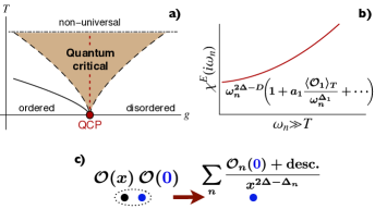
Figure 1: a) Phase diagram near a quantum critical point (QCP). b) Asymptotic behavior of the Euclidean susceptibility associated with an operator $\mathcal{O}$ of scaling dimension $\Delta$: $\chi^{\rm E}(i\omega_{n})=\langle\mathcal{O}(-\omega_{n})\mathcal{O}(\omega_{n})\rangle_{T}$. c) Schematic operator product expansion (OPE) determining the asymptotics of $\chi$. “desc.” denotes the descendants of the primary $\mathcal{O}_{n}$ (dimension $\Delta_{n}$).

Asymptotics and OPE: We consider a thermally excited system tuned to a QC point via a non-thermal parameter $g$. In the phase diagram Fig. 1a, this corresponds to the line in the QC fan at $g\!=\!g_{c}$ and $T\geq 0$. We are interested in the linear-response dynamics at finite temperature, more precisely in the retarded dynamical susceptibility associated with a bosonic observable $\mathcal{O}$, such as the energy or charge density: $\chi^{R}(t,{\bf x})=-i\Theta(t)\left\langle\left[\mathcal{O}(t,{\bf x}),\mathcal{O}(0,{\bf 0})\right]\right\rangle_{T}$, where the average is taken over the thermal ensemble. We set $\hbar=k_{B}=c=1$; $c$ is the characteristic speed near the QC point. We will often work in Fourier space: $\chi^{R}(\omega,{\bf k})=\int\!{\rm d}t{\rm d}^{d}{\bf x}\chi^{R}(t,{\bf x})e^{i\omega t-i{\bf k}\cdot{\bf x}}$, where $\omega$ is the real frequency and ${\bf k}$ the momentum. Using $T$, the only energy scale available, $\chi^{R}$ can be rewritten to make its scaling properties manifest:

$$\chi^{R}(\omega,{\bf k})=T^{2\Delta_{\mathcal{O}}-D}\,\Phi\!\left(\frac{\omega}{T},\frac{{\bf k}}{T^{1/z}}\right)\,,$$ (1)

where $\Delta_{\mathcal{O}}$ is the scaling dimension of $\mathcal{O}$, $\Phi$ is a universal scaling (complex) function, and $z$ the dynamical critical exponent. This scaling structure emerges at low energies, i.e. $\omega,|{\bf k}|,T\ll\Lambda_{\rm UV}$, where $\Lambda_{\rm UV}$ is a microscopic lattice energy scale, represented by the horizontal dot-dashed line in Fig. 1a. We emphasize that in this regime the ratios $(\omega,|{\bf k}|^{z})/T$ can be arbitrary. We introduce the corresponding universal response function

$$\mathcal{R}(\omega,{\bf k})=\frac{\chi^{R}(\omega,{\bf k})}{i\omega-0^{+}}\,,$$ (2)

using the Kubo prescription. E.g. if $\mathcal{O}=J_{x}$ is a conserved current, $\chi_{xx}^{R}$ is the $xx$-polarization function and $\mathcal{R}_{xx}(\omega,{\bf 0})=\sigma_{xx}(\omega)$ the dynamical conductivity. Due to the strong interactions and the resulting absence of quasiparticles in generic QC systems, little is known about these universal responses, and our goal is to unravel some of their robust properties. First, let us begin with the large-frequency regime, $\omega\gg T,|{\bf k}|$, where the dynamics are near those of the groundstate. These can be elegantly studied via the operator product expansionWilson (1969) (OPE) of $\mathcal{O}$ with itself. The OPE is an operator relation and does not depend on temperature. For a general QFT, it is a short time/distance expansion that captures the behavior of the operator product $\mathcal{O}_{1}(t,{\bf x})\mathcal{O}_{2}(0,{\bf 0})$ as $t,|{\bf x}|\rightarrow 0$, which by locality, can be expressed as an infinite sum of operators evaluated at $t,|{\bf x}|=0$. We will mostly focus on CFTs, which have $z=1$ and describe a large class of experimentally relevant QC phase transitions such as those in the quantum Ising and XY models. In a CFT, the $\mathcal{O}\mathcal{O}$ OPEFerrara et al. (1972); Polyakov (1974) of a primary operator $\mathcal{O}$ with scaling dimension $\Delta_{\mathcal{O}}$ reads (Fig. 1c)

$$\mathcal{O}(x)\mathcal{O}(0)=\sum_{\mathcal{O}_{n}\,{\rm primary}}\!\frac{C_{n}\big{(}x,\tfrac{\partial}{\partial y}\big{)}}{|x|^{2\Delta_{\mathcal{O}}-\Delta_{n}}}\mathcal{O}_{n}(y)\Big{|}_{y=0}\,,$$ (3)

which is expressed in imaginary time $\tau$: $|x|^{2}=\tau^{2}+{\bf x}^{2}$. A primary operator transforms homogeneously under conformal transformations; e.g. conserved currents and the order parameter in the O$(N)$ model. The sum in Eq. (3) is over primaries $\mathcal{O}_{n}$ with scaling dimensions $\Delta_{n}$; it includes the identity (dimension 0). The differential operator $C_{n}\big{(}x,\tfrac{\partial}{\partial x}\big{)}$ is homogeneous under $x\rightarrow bx$, and encodes the contributions from the descendants of $\mathcal{O}_{n}$ (obtained by applying derivatives to $\mathcal{O}_{n}$). Going to Fourier space and taking a thermal expectation value (TEV) we obtain a key result (Fig. 1b): the $|k|\gg T$ behavior of the Euclidean susceptibility,

$$\chi^{\rm E}(k)=|k|^{2\Delta_{\mathcal{O}}-D}\!\!\!\sum_{\mathcal{O}_{n}\,{\rm primary}}\!\!\!\left(c_{n}(k)\frac{\langle\mathcal{O}_{n}\rangle_{T}}{|k|^{\Delta_{n}}}+\dotsb\right)\,,$$ (4)

where $|k|^{2}=\omega_{n}^{2}+{\bf k}^{2}$, $\omega_{n}=2\pi Tn$ is a Matsubara frequency. The dimensionless functions $c_{n}$ encode the appropriate $k$-space tensor structure (and can contain logarithms). The dots correspond to higher powers of $T/|k|$ arising from the descendants of $\mathcal{O}_{n}$. Crucially, a scaling operator will acquire a TEV, $\langle\mathcal{O}_{n}\rangle_{T}=d_{n}\,T^{\Delta_{n}}$, since $T$ is the only energy scale. $d_{n}$ is a universal real number. Substituting this into Eq. (4) we obtain a general expression for the large-$k$ asymptotic expansion of $\chi$. We see that the lowest dimension operators appearing in the OPE dictate how the susceptibility approaches its groundstate value as $T/|k|\rightarrow 0$. To obtain the real quantum dynamics, we can analytically continue the imaginary frequency expansion Eq. (4) to real frequencies termwise, with the replacement $i\omega_{n}\!\to\omega+i0^{+}$. This follows from the structure of the OPE and the spectral representation connecting the Euclidean and retarded susceptibilities (see App. A for an extension of the proof in [Caron-Huot, 2009]).

Interestingly, unitarity and conformal symmetry constrain the scaling dimensions of these operatorsMack (1977): $\Delta_{n}\geq(D-2)/2$. This leads to important inequalities for dynamical susceptibilities. Let us work in 2+1D and consider a putative low-energy susceptibility $\chi(\omega)$ obtained from an experiment or simulation, and express it as

$$\chi(\omega)\overset{\omega\gg T}{=}\omega^{2\delta_{1}-3}\,\bigg{[}a+b\left(\frac{T}{\omega}\right)^{\!\delta_{2}}+\dotsb\bigg{]}\,,$$ (5)

at large frequencies. Finding either $\delta_{i}<1/2$ would violate unitarity bounds and thus rule out a conformal QC pointMaldacena . For Wilson-Fisher QC points, we shall see that the stronger condition, $\delta_{2}>1.4$, holds. Before applying the above general results to those CFTs, we discuss how the asymptotics can be used to prove sum rules for any susceptibility (2-point function).

Sum rules: We put forth a powerful sum rule for the real frequency quantum dynamical response function:

$$\int_{-\infty}^{\infty}\!\frac{d\omega}{\pi}\operatorname{Re}\delta\mathcal{R}(\omega,{\bf k})=-\delta\chi^{\infty}\,.$$ (6)

$\delta\mathcal{R}$ is defined as in Eq. (2), with a modified susceptibility $\chi\!\to\!\delta\chi$, defined below. The sum rule is independent of small frequency details, and fundamentally relies on the retarded causal structure of $\chi^{R}$. More precisely it is the zero-frequency limit of the Kramers-Kronig transform for the modified susceptibility, $\delta\chi^{R}(\omega,{\bf k})-\delta\chi^{\infty}$, which we now discuss. In the QC scaling regime, $\chi$ does not usually decay at large frequencies unlike on the lattice because it encodes excitations at all scales. To formulate the sum rule, we thus generally need to subtract terms, denoted by $\tilde{\chi}$, from $\chi$ to remove its large-$\omega$ divergenceGulotta et al. (2011); Witczak-Krempa and Sachdev (2012, 2013); Witczak-Krempa (2014): $\delta\chi(\Omega,{\bf k})=\chi(\Omega,{\bf k})-\tilde{\chi}(\Omega)$, where $\Omega$ is a complex frequency in the upper half-plane. In some cases, one further needs to subtract a remaining constant: $\delta\chi^{\infty}=\delta\chi^{\rm E}(\Omega\!\to\!i\infty,{\bf k})$, where the limit is taken at fixed $T$. We emphasize that $\tilde{\chi}(\Omega)$ is momentum-independent because the asymptotic behavior Eq. (4) depends on powers of $T/\sqrt{\omega_{n}^{2}+|{\bf k}|^{2}}$ due to the asymptotic re-emergence of Lorentz invariance (broken by $T$), and we fix ${\bf k}$ as we take $\omega_{n}\gg T$. We note that the correlation functions studied here only depend on the magnitude of the momentum $|{\bf k}|$, which implies that $\operatorname{Im}\chi^{R}$,$\operatorname{Re}\mathcal{R}$ are $\omega$-even functions, so that the integral Eq. (6) can be written for $\omega\geq 0$.

The highly non-trivial and theory dependent information is contained in the subtraction terms $\tilde{\chi},\delta\chi^{\infty}$ which are determined from the large-frequency behavior, i.e. from the leading terms in OPE, Eq. (3). We now derive some general properties of the subtractions. First, the main subtraction $\delta\chi=\chi-\tilde{\chi}$ is generally required because the leading asymptotic $|k|\gg T$ behavior of $\chi^{\rm E}(k)$ is $|k|^{2\Delta_{\mathcal{O}}-D}$, and most operators have $2\Delta_{\mathcal{O}}>D$. In contrast, in almost all cases the subtraction of a constant is not needed, i.e. $\delta\chi^{\infty}=0$. Indeed, from Eq. (4) this constant can be non-zero only if the $\mathcal{O}\mathcal{O}$ OPE contains an operator $\mathcal{O}_{*}$ with dimension $\Delta_{*}=2\Delta_{\mathcal{O}}-D$. Moreover, $\mathcal{O}_{*}$ needs to have a non-zero TEV. In which case, $\delta\chi^{\infty}\propto\langle\mathcal{O}_{*}\rangle_{T}$ and the constant of proportionality is the corresponding OPE coefficient. A further necessary condition for $\delta\chi^{\infty}\neq 0$ is $\Delta_{\mathcal{O}}\geq(3D-2)/4$ because of the unitarity boundMack (1977) on $\Delta_{*}$. A generic case where the subtraction $\delta\chi^{\infty}$ appears is for a 2-point function of $T_{\mu\nu}$, the stress tensor, because the latter has scaling dimension $D$. In this case $\mathcal{O}_{*}\!=\!T_{\mu\nu}$ since the stress tensor generally appears in the $T_{\mu\nu}T_{\lambda\varepsilon}$ OPE. Below we will the consequences of this for the shear viscosity.

O$(N)$ model: We now apply the above general results to the QC point of the quantum O$(N)$ modelpol (1987); Sachdev (2011) in dimensions $2<D<4$. This is the famous Wilson-Fisher conformal fixed point. It describes a variety of experimentally relevant quantum phase transitions: Ising ($N\!=\!1$), XY ($N\!=\!2$), etc. An exact solution exists at $N\!=\!\infty$, which we will use to perform non-trivial checks. As a field theory, the O$(N)$ (non-linear sigma) model is defined by the action $S=\int\!{\rm d}^{D}\!x\frac{1}{g}\partial_{\mu}\varphi_{a}\partial_{\mu}\varphi_{a}$, where $\varphi_{a}(x)$ is a real $N$-component vector field of fixed norm $\varphi_{a}\varphi_{a}=1$. As the coupling $g$ is increased the system undergoes a QC phase transition at $g=g_{c}$ from a broken symmetry phase to a symmetric one for $g>g_{c}$ (Fig. 1a).

For our asymptotics/sum rule analysis we need the list of operators $(\mathcal{O}_{n},\Delta_{n})$ with low dimensions $\Delta_{n}\leq D$. These are known from large-$N$ and small $(4-D)$ expansionsZinn-Justin (2002); Pelissetto and Vicari (2002), Monte CarloPelissetto and Vicari (2002), non-perturbative bootstrapEl-Showk et al. (2012); Kos et al. (2014); El-Showk et al. (2014a), etc. The first one being the order parameter field $\phi_{a}$ with dimension $\Delta_{\phi}=(D-2+\eta_{\phi})/2$, where $\eta_{\phi}$ is the field’s anomalous dimension. The following O$(N)$-invariant operators will also appear: the “thermal” operator $(\mathcal{O}_{\!g},\Delta_{g})$, the conserved currents $(J^{\mu}_{ab},D-1)$, and the stress tensor $(T_{\mu\nu},D)$. The dimensions of the currents and stress tensor receive no anomalous corrections because they are protected by symmetries. The operator $\mathcal{O}_{\!g}$ (often denoted by $\varepsilon$ in the context of the Ising model) is associated with the Lagrange multiplier field $\lambda(x)$ that constrains $\varphi_{a}\varphi_{a}=1$ in the O$(N)$ model. It has dimension $\Delta_{g}=D-1/\nu$, where $\nu$ is the correlation length exponent; for the $D\!=\!3$ Ising casePelissetto and Vicari (2002); El-Showk et al. (2012), $\Delta_{g}=1.413$. It is directly related to the singlet $\phi^{2}$, and tunes the system away from the QC point. Being the only relevant O$(N)$-symmetric scalar, it is the most important operator as it dominates the asymptotic quantum dynamics: we will see that it generally gives the first finite-$T$ correction. This was recently shownKatz et al. (2014) to be the case for the conductivity of the O$(N)$ model, and observed numericallyKatz et al. (2014) for $N=2$. Given the generality of our OPE analysis, we infer that this “dominance” of the relevant symmetric scalar is a generic property of QC transitions.

Order parameter susceptibility: We first study $\chi_{ab}(k)=\langle\phi_{a}(-k)\phi_{b}(k)\rangle_{T}$, i.e. the order parameter susceptibility. It is one of the simplest observables, and yields the low-energy staggered spin susceptibility of quantum antiferromagnets with transitions in the O$(N)$ universality class. We begin by analyzing its asymptotics. By symmetry, and from the knowledge of the operators with low dimensions we can write the leading terms in the $\phi_{a}\phi_{b}$ OPE:

$$\phi_{1}(x)\phi_{1}(0)\!=\!\frac{C_{\phi}}{x^{2\Delta_{\phi}}}+\frac{C_{\!\phi\phi g}\mathcal{O}_{\!g}(0)}{x^{2\Delta_{\phi}-\Delta_{g}}}+\frac{C_{\!\phi\phi T}x_{\mu}x_{\nu}T_{\mu\nu}(0)}{x^{2\Delta_{\phi}-D+2}}+\dotsb$$ (7)

where we focus on $a,b=1$ since $\chi_{ab}$ is diagonal by virtue of O$(N)$ symmetry. We have omitted the contribution from the currents $J^{\mu}_{ab}$ because they have vanishing TEV (no excess charge or net current in the thermal ensemble). Taking the TEV of Eq. (7) gives the asymptotic behavior

$$\chi_{11}^{\rm E}(i\omega_{n},{\bf k})=|k|^{2\Delta_{\phi}-D}\bigg{[}\mathcal{C}_{\phi}+\mathcal{C}_{\phi\phi g}d_{g}\left|\frac{T}{k}\right|^{\Delta_{g}}\\ +\mathcal{C}_{\phi\phi T}\frac{k_{\mu}k_{\nu}}{k^{2}}d_{T}^{\mu\nu}\left|\frac{T}{k}\right|^{D}+\dotsb\bigg{]}\,.$$ (8)

$C_{\#}/\mathcal{C}_{\#}$ in Eqs. (7)/(8) are real OPE coefficients in position/momentum space, which can be obtained from groundstate 3-point functions. As anticipated, the first subleading term comes from the relevant scalar $\mathcal{O}_{\!g}$. The next term arises from the stress tensor, where $\langle T_{\mu\nu}\rangle_{T}=d_{T}^{\mu\nu}T^{D}$ is diagonal. At $N=\infty$, $\Delta_{\phi}=(D-2)/2$ saturates the unitarity bound, but finite $N$ fluctuations lead to a small anomalous dimension $\eta_{\phi}\ll 1$Zinn-Justin (2002); Pelissetto and Vicari (2002); El-Showk et al. (2012); Kos et al. (2014). The OPE coefficients $\mathcal{C}_{\phi\phi g},\mathcal{C}_{\phi\phi T}$ are generally finite and can be computed using a $1/N$ expansion for instance. $C_{\phi\phi g}$ has been computed using bootstrapEl-Showk et al. (2014b) and Monte CarloCaselle et al. (2015) for $N\!\!=\!1$. From the above expansion, we can derive the sum rule for $\chi_{ab}$. First, for any $N$, $\chi_{ab}$ decays sufficiently fast at large frequencies so that the subtractions vanish, $\tilde{\chi}_{ab}=\delta\chi_{ab}^{\infty}=0$, and the sum rule takes its simplest form:

$$\int_{0}^{\infty}\!{\rm d}\omega\operatorname{Re}\mathcal{R}_{ab}(\omega,{\bf k})=0\,,$$ (9)

where $\mathcal{R}_{ab}(\omega,{\bf k})=\chi_{ab}^{R}(\omega,{\bf k})/(i\omega-0^{+})$ is the response.

When $N=\infty$, we have the exact solution for $2<D<4$: $\chi_{ab}^{\rm E}(i\omega_{n},{\bf k})=\delta_{ab}/(\omega_{n}^{2}+{\bf k}^{2}+m_{T}^{2})$, where $m_{T}=\Theta_{d}T$ is the thermal mass, and $\Theta_{d}$ is a positive numberPetkou and Vlachos (1998), see App. B. Expanding for $|k|\gg T$, we get $\chi_{ab}^{\rm E}(k)=\tfrac{1}{k^{2}}\big{[}1-(\tfrac{m_{{}^{T}}}{k})^{2}+(\tfrac{m_{{}^{T}}}{k})^{4}+\dotsb\!\big{]}$. In agreement with the OPE, Eq. (7), the subleading term $-m_{T}^{2}/k^{4}$ has $\Delta_{g}^{\!N=\infty}\!=2$ (i.e. $1/\nu\!=\!\!D-2$) and is proportional to $\langle\mathcal{O}_{\!g}\rangle_{T}=\sqrt{N}m_{T}^{2}$. This later TEV is evaluatedKatz et al. (2014) in the $N\!=\!\infty$ limit. We note the absence of a contribution from the stress tensor, $\sim m_{T}^{3}/|k|^{5}$. Although the real-space OPE coefficient $C_{\phi\phi T}$ in Eq. (7) is non-zero, upon Fourier transforming to $k$-space, that term does not contribute to the large-$k$ behavior. This is an artefact of $N=\infty$, where $\phi$ has no anomalous dimension. Finally, the sum rule Eq. (9) can be easily checked as the spectral function is a sum of (quasiparticle) delta functions.

Scalar susceptibility: The scalar susceptibility $\chi_{s}$ is the 2-point function of the “thermal” operator, $\langle\mathcal{O}_{\!g}(-k)\mathcal{O}_{\!g}(k)\rangle_{T}$. It has recently been the focus of attention in the study of the amplitude “Higgs” modeEndres et al. (2012); Pollet and Prokof’ev (2012); Podolsky and Sachdev (2012); Gazit et al. (2013); Rançon and Dupuis (2014); Tenenbaum Katan and Podolsky (2014). Again, we first examine the $\mathcal{O}_{\!g}\mathcal{O}_{\!g}$ OPE. The terms relevant here are given, mutatis mutandis, by Eq. (7). This then leads to the large-$k$ expansion Eq. (8) with $(\phi_{a},\Delta_{\phi})$ replaced by $(\mathcal{O}_{\!g},\Delta_{g})$. With this data, we can derive the sum rule for $\chi_{s}$. First, $\delta\chi_{s}^{\infty}=0$ since there is no O$(N)$-singlet with dimension $\Delta_{*}=2\Delta_{g}-D$ in the spectrum. The other ingredient needed to build the sum rule is the term removing the large-$\omega$ divergence, $\tilde{\chi}_{s}$. In this case, it is simply the groundstate value of $\chi_{s}$ at ${\bf k}\!=\!{\bf 0}$: $\tilde{\chi}_{s}(\Omega)=\chi_{s}^{T=0}(\Omega,{\bf 0})=\mathcal{C}_{g}\Omega^{2\Delta_{g}-D}$. The sum rule reads:

$$\int_{0}^{\infty}\!{\rm d}\omega\operatorname{Re}[\mathcal{R}_{s}(\omega,{\bf k})-\mathcal{R}_{s}^{T=0}(\omega,{\bf 0})]=0\,.$$ (10)

We can again carry out the asymptotic analysis exactly for $N\!\to\!\!\infty$. The result is (App.  B): $\chi_{s}^{\rm E}(k)=-\frac{N}{a_{0}}\,|k|^{4-D}(1-a_{g}|\tfrac{T}{k}|^{2}-a_{T}|\frac{T}{k}|^{D}+\dotsb)$, where $a_{\#}$ are $D$-dependent constants. Interestingly, the coefficient of the subleading term, $a_{g}$, vanishes exactly for $D=3$. This comes from the somewhat surprising fact that the thermal operator $\mathcal{O}_{\!g}$ does not appear by itself in the $\mathcal{O}_{\!g}\mathcal{O}_{\!g}$ OPE when $D=3$ in the $N\!=\!\infty$ limit. In other words, the $C_{\!ggg}^{D=3}$ OPE coefficient vanishes. This does not happen for $D\neq 3$, and we do not expect it to hold at finite $N$ in $D=3$. Indeed, for the Ising case this coefficient was recently computed using Monte Carlo methods and found to be finiteCaselle et al. (2015). Finally, the sum rule Eq. (10) can be checked numerically at $N\!=\!\infty$ (App. B).

Dynamical shear viscosity: Finally we examine a correlator involving the stress tensor. Not only is this of fundamental interest because it can be defined for any CFT, but it will also reveal the full complexity of the sum rule. We consider the dynamical shear viscosity, $\eta(\omega,{\bf k})=\chi^{R}_{\eta}(\omega,{\bf k})/(i\omega-0^{+})$, obtained from the $T_{xy}$ 2-point function, $\chi_{\eta}^{R}$. $T_{xy}$ measures the flux of $x$-momentum in the $y$-direction, and $\eta$ probes the system’s resistance against momentum gradients. The asymptotic behavior of $\eta$ follows from the $T_{xy}T_{xy}$ OPE, which we here formulate in momentum space:

$$\lim_{|k|\gg|p|}T_{xy}(k)T_{xy}(-k+p)=\mathcal{C}_{T}|k|^{D}\delta(p)\\ +\mathcal{C}_{TTg}|k|^{D-\Delta_{g}}\mathcal{O}_{\!g}(p)+C_{TTT}^{\mu\nu}T_{\mu\nu}(p)+\dotsb\,,$$ (11)

where here ${\bf k}=0$ for simplicity. This can then be used to derive a sum rule for $\eta$, which is more involved than for the response functions considered above. For one, $\delta\chi_{\eta}^{\infty}=\!\mathcal{C}_{TTT}^{\mu\nu}\langle T_{\mu\nu}\rangle_{T}$ is non-zero, as was explained above on general grounds for 2-point functions involving $T_{\mu\nu}$. Second, the subtraction involved in $\delta\chi_{\eta}$ is temperature dependent because $\mathcal{O}_{\!g}$ is relevant. This leads to the following sum rule for the shear response:

$$\int_{0}^{\infty}\!\!\!{\rm d}\omega\operatorname{Re}\!\big{[}\eta(\omega,{\bf k})-\mathcal{C}_{T}\omega^{d}-\mathcal{A}(\omega/i)^{d-\Delta_{g}}\big{]}=c_{\eta}P\,,$$ (12)

where $d=D-1$, $\mathcal{A}=\mathcal{C}_{TTg}\langle\mathcal{O}_{\!g}\rangle_{T}$, $P=\langle T_{xx}\rangle_{T}$ is the pressure of the CFT, and $c_{\eta}=-\pi\delta\chi_{\eta}^{\infty}/(2P)$ is a dimensionless constant. The second term in the integrand is $\eta^{T=0}(\omega,{\bf 0})$ and mirrors the subtraction in the scalar sum rule. The third one depends on temperature via $\mathcal{A}\propto T^{\Delta_{g}}$ and scales with a non-trivial $\omega$ power depending on the correlation length exponent $\nu$ via $\Delta_{g}=D-1/\nu$. Some QC theories are simpler in that they lack a relevant scalar that condenses at $T>0$, as we now discuss.

We contrast the above shear sum rule with the simpler ones obtainedRomatschke and Son (2009); Caron-Huot (2009) for $\mathcal{N}=4$ super Yang-Mills and pure Yang-Mills, which are gauge theories in $D\!=\!4$. In those cases, the result is as in Eq. (12) except that the third term in the integrand is absent. This stems from the fact that those theories do not contain a symmetric relevant scalar like $\mathcal{O}_{\!g}$, i.e. they are not realized by fine tuning a symmetric “mass” term. The massless version of QED in $D=3$ with many Dirac fermions coupled to a U(1) gauge field also satisfies this property, being a stable phase. It will thus have a shear sum rule of the same form as super Yang-Mills. Finally, we note that shear sum rules analogous to Eq. (12) were derived in the context of strongly interacting ultracold Fermi gasesTaylor and Randeria (2010); Enss et al. (2011); Goldberger and Khandker (2012), which generally do not have emergent Lorentz symmetry.

Outlook: Our non-perturbative results, via the operator product expansion (OPE), for the asymptotics and sum rules apply to a wide class of conformal QC points, many of which describe experimentally relevant systems. It will be interesting to apply the program described in this article to theories other than to the O$(N)$ Wilson-Fisher fixed point, treated here, or even to non-conformal QC systems. The strong constraints we have derived will also be useful for the analysis of numerical and experimental data. For instance, quantum Monte Carlo is a powerful tool to study QC dynamics in imaginary timeŠmakov and Sørensen (2005); Witczak-Krempa et al. (2014); Katz et al. (2014); Chen et al. (2014); Swanson et al. (2014); Gazit et al. (2014), and can be used to study the asymptotic regime where the OPE analysis applies, as was recently shownKatz et al. (2014) for the conductivity. The asymptotics and sum rules will also help with the difficult task of analytically continuing the imaginary time data to real time by constraining the allowed scaling functions. Along those lines, our results can be used with a novel methodWitczak-Krempa et al. (2014); Katz et al. (2014) of analytic continuation based on the AdS/CFT holographic principleMaldacena (1998): Specific data about a QC theory can be encoded in holographic physically-motivated Ansatzes for the scaling functions. These can then be used to perform the continuation.

Acknowledgments: I am indebted to E. Katz, S. Sachdev, and E.S. Sørensen for their collaboration on related topics. I further acknowledge stimulating exchanges with D.J. Gross, C. Herzog, J. Maldacena, R. Myers and D.T. Son. Research at Perimeter Institute is supported by the Government of Canada through Industry Canada and by the Province of Ontario through the Ministry of Research and Innovation.

Supplementary Information

Appendix A Analytic continuation of asymptotic susceptibility

This appendix explains how the quantum critical (QC) dynamics in the near groundstate regime follow from the operator product expansion (OPE) in imaginary time. More precisely, we show that the asymptotics at large real frequencies, $\omega\gg T$, can be obtained from the Euclidean frequency result via term by term analytic continuation. To do so, we adapt the line of reasoning put forth in Ref. Caron-Huot, 2009. The analysis begins with the spectral representation for the Euclidean susceptibility:

$$\chi^{\rm E}(i\Omega)=\int_{-\infty}^{\infty}\frac{{\rm d}\omega^{\prime}}{\pi}\frac{\rho(\omega^{\prime})}{\omega^{\prime}-i\Omega}\,,$$ (13)

where $\rho(\omega)=\operatorname{Im}\chi^{R}(\omega+i0^{+})$ is the spectral density of the retarded 2-point function. We have dropped the momentum dependence of $\rho$ and any other indices as these are not crucial to the discussion. Here $\Omega>0$ so that $i\Omega$ is a positive frequency along the imaginary axis, so that taking a principal value of the integral is not necessary. At finite temperature we should strictly speaking use Matsubara frequencies, $\Omega=\omega_{n}=2\pi Tn$, in Eq. (13). However, it is more convenient to employ the spectral representation to analytically continue the susceptibility to arbitrary frequencies along the imaginary axis, and more generally to the upper half of the complex plane. In writing the above equation, we have assumed that $\rho(\omega)$ vanishes as $|\omega|\to\infty$. If this fails one needs to use a subtracted density, $\delta\rho=\operatorname{Im}\delta\chi^{R}$, as was discussed in the main text. Our argument is independent of this complication, on which we shall comment towards the end of the section.

For the cases of interest, namely 2-point functions of bosonic operators, $\rho(\omega)$ is $\omega$-odd allowing us to reduce the integral to positive frequencies:

$$\chi^{\rm E}(i\Omega)=\int_{0}^{\infty}\frac{{\rm d}\omega^{\prime}}{\pi}\frac{2\omega^{\prime}}{\omega^{\prime 2}+\Omega^{2}}\rho(\omega^{\prime})\,.$$ (14)

We use the convention according to which $\rho(\omega)$ is positive for $\omega>0$. Now, assuming that $\rho(\omega)$ has a large-frequency expansion in powers of $1/\omega$, we will show that it leads to a corresponding expansion in powers of $1/\Omega$ for $\chi^{\rm E}(i\Omega)$. Logarithms can appear but do not spoil the correspondence, see Sec. A.1. Let us assume that $\rho(\omega)$ is bounded by the tail $1/\omega^{\epsilon}$, $0<\epsilon<1$, at large frequencies. Using the positivity of Eq. (14), one can show that $\chi^{\rm E}$ is bounded by $1/\Omega^{\epsilon}$ as $\Omega\to\infty$, and thus vanishes in that limit. It can also be shown that the first derivative of Eq. (14) with respect to $1/\Omega$ diverges as $\Omega\to\infty$. This establishes that $\chi^{\rm E}\to 1/\Omega^{\bar{\epsilon}}$ at large $\Omega$, with an exponent $0<\bar{\epsilon}\leq\epsilon$. The procedure can be adapted to a more general spectral tail, $1/\omega^{\ell+\epsilon}$, where $\ell$ is a positive integer. In this case, one needs to take $\ell+1$ derivatives with respect to $1/\Omega$. The argument can be further iterated for all the terms in the power law expansion of $\rho$ by considering a modified density $\tilde{\rho}$ from which one has subtracted terms up to the one that is targeted. We have thus established that an expansion for $\rho$ in powers of $1/\omega$ leads to a corresponding expansion in powers for $\chi^{\rm E}$. We now turn to the crux of the proof and show that these expansions are precisely related by termwise analytic continuation, $i\Omega\leftrightarrow\omega+i0^{+}$.

Let us assume that $\rho(\omega)$ contains the power law $1/\omega^{\alpha}$ for $\omega\gg\omega_{0}$, where we are mainly interested in the case where the infrared scale is temperature, $\omega_{0}=T$. Consider $\alpha>0$ but not an even integer, then using Eq. (14) we get

$$\int_{\omega_{0}}^{\infty}\frac{{\rm d}\omega^{\prime}}{\pi}\frac{2\omega^{\prime}}{\omega^{\prime 2}+\Omega^{2}}\,\frac{1}{\omega^{\prime\alpha}}=\frac{1}{\Omega^{\alpha}\sin(\pi\alpha/2)}+\frac{2}{\pi}\sum_{n=1}a_{n}\frac{\omega_{0}^{2n-\alpha}}{\Omega^{2n}}\,,$$ (15)

where $a_{n}=(-1)^{n+1}/(\alpha-2n)$. We see that the first term is the expected power law, and is independent of the infrared scale $\omega_{0}$ defining the asymptotic regime. The remaining terms depend on $\omega_{0}$ and form a series that contains only even powers of $1/\Omega$. Due to their incompatible powers, these do not interfere with the first term. In addition, the factor of $1/\sin(\pi\alpha/2)$ is exactly as expected from the analytic continuation:

$$\Omega^{-\alpha}\leftrightarrow(-i\omega+0^{+})^{-\alpha}=\omega^{-\alpha}[\cos(\pi\alpha/2)+i\sin(\pi\alpha/2)]\,.$$ (16)

We can also recover the real part of $\chi^{R}$ by making use of the Kramers-Kronig transform (an application of the spectral representation),

$$\operatorname{Re}\chi^{R}(\omega+i0^{+})=\mathcal{P}\!\!\int_{0}^{\infty}\frac{{\rm d}\omega^{\prime}}{\pi}\frac{2\omega^{\prime}\rho(\omega^{\prime})}{\omega^{\prime 2}-\omega^{2}}\,,$$ (17)

where we have again made use of the fact that $\rho(\omega)$ is odd. $\mathcal{P}\!\!\int$ denotes the principal value of the integral. Using an infrared cutoff $\omega_{0}$, we find that the real part corresponding to a spectral power law tail $1/\omega^{\alpha}$ is

$$\operatorname{Re}\chi^{R}(\omega+i0^{+}) \to\mathcal{P}\!\!\int_{\omega_{0}}^{\infty}\frac{{\rm d}\omega^{\prime}}{\pi}\frac{2\omega^{\prime}}{\omega^{\prime 2}-\omega^{2}}\frac{1}{\omega^{\prime\alpha}}$$ (18)

$$=\frac{\cot(\pi\alpha/2)}{\omega^{\alpha}}-\frac{2}{\pi}\sum_{n=1}b_{n}\frac{\omega_{0}^{2n-\alpha}}{\omega^{2n}}$$ (19)

where $\cot x=\cos(x)/\sin(x)$, and $b_{n}=1/(\alpha-2n)$. The first term is independent of $\omega_{0}$ and precisely yields the answer expected from Eq. (16), whereas the remaining series again decouples because it only contains even powers of $1/\omega$.

In the above, we have assumed that $\rho(\omega)$ decays to zero as $\omega\to\infty$. If this is not the case, one can analytically continue the terms with positive powers of $\omega$ using Eq. (16), and apply the above procedure to the modified susceptibility, $\chi-\tilde{\chi}-\delta\chi^{\infty}$, which vanishes as $\omega\to\infty$. We refer the reader to the main text for a detailed discussion regarding the subtractions $\tilde{\chi},\delta\chi^{\infty}$. We have thus shown that the asymptotic expansions of the retarded and Euclidean susceptibilities are precisely related by a termwise analytic continuation.

Our results can be explicitly checked for the infrared fixed point of the O$(N)$ model in the $N\to\infty$ limit, as is discussed in the main text and in the next appendix. In the context of the charge conductivity in 2+1D, this was done for the O$(N\to\infty)$ model and the Dirac CFT in Ref. Katz et al., 2014, and for a wide class of conformal QC theories without quasiparticles using AdS/CFT in Refs. Katz et al., 2014; Witczak-Krempa, 2014; Gulotta et al., 2011.

A.1 Even powers in the spectral function

We now turn to the more subtle case of even powers in $\rho(\omega)$. From the basic formula for analytic continuation, Eq. (16), we see that even powers in imaginary frequencies contribute only to the real part of $\chi^{R}$. E.g. $1/\Omega^{2}\to-1/\omega^{2}$, which does not contribute to $\rho=\operatorname{Im}\chi^{R}$. To understand what asymptotic Euclidean term can give rise to a $1/\omega^{2}$ scaling for $\rho$, we turn to the spectral representation, Eq. (14),

$$\int_{\omega_{0}}^{\infty}\frac{{\rm d}\omega^{\prime}}{\pi}\frac{2\omega^{\prime}}{\omega^{\prime 2}+\Omega^{2}}\,\frac{1}{\omega^{\prime 2}} =\frac{1}{\pi\Omega^{2}}\ln\left(1+\frac{\Omega^{2}}{\omega_{0}^{2}}\right)\,;$$ (20)

$$\overset{\Omega\gg\omega_{0}}{=}\frac{\ln\left(\frac{\Omega^{2}}{\omega_{0}^{2}}\right)}{\pi\Omega^{2}}+\frac{1}{\pi}\sum_{n=2}r_{n}\frac{\omega_{0}^{2n-2}}{\Omega^{2n}}\,,$$ (21)

where $\omega_{0}$ is the infrared cutoff we have employed above, and $r_{n}=(-1)^{n}/(n-1)$. The first term decouples from the series due to the presence of the logarithm; also note that there is no $1/\Omega^{2}$ term in the series. We thus see that a logarithm in $\chi^{\rm E}$ gives rise to a $1/\omega^{2}$ term in $\rho$. This is fully consistent with the direct analytic continuation of the term with the logarithm:

$$\frac{\ln\left(\frac{\Omega^{2}}{\omega_{0}^{2}}\right)}{\pi\Omega^{2}}\;\xrightarrow{i\Omega\to\omega+i0^{+}}\;-\frac{\ln\left(\frac{\omega^{2}}{\omega_{0}^{2}}\right)}{\pi\omega^{2}}+\frac{i}{\omega^{2}}\,,$$ (22)

for $\omega>0$. Analogous results hold for higher powers of $1/\omega$, e.g. $1/\omega^{4}$ obtains from $(\pi\Omega^{4})^{-1}\ln(\Omega^{2}/\omega_{0}^{2})$, etc. We note that such logarithms do not appear in the leading expansion of the response functions of the Wilson-Fisher QC points studied in this paper.

Appendix B Scalar susceptibility of the O$(N)$ model at large $N$

We give details regarding the asymptotics and sum rule for the scalar susceptibility $\chi_{s}(k)=\langle\mathcal{O}_{\!g}(-k)\mathcal{O}_{\!g}(k)\rangle_{T}$ of the O$(N$) Wilson-Fisher fixed point in the large $N$ limit. Using the O$(N)$ non-linear sigma model defined in the main text, it can be shownSachdev (2011) that for $N\to\infty$ the susceptibility is given by

$$\chi_{s}(k)=-\frac{N}{\Pi(k)}\,,$$ (23)

with the scalar polarization function

$$\Pi^{\rm E}(i\omega_{n},{\bf k})=T\sum_{\nu_{n}}\int\frac{{\rm d}^{d}{\bf q}}{(2\pi)^{d}}\chi_{11}^{\rm E}(i\omega_{n}+i\nu_{n},{\bf k}+{\bf q})\chi_{11}^{\rm E}(i\nu_{n},{\bf q})\,.$$ (24)

The sum/integral involves

$$\chi_{ab}^{\rm E}(k)=\frac{\delta_{ab}}{\omega_{n}^{2}+{\bf k}^{2}+m_{T}^{2}}\,,$$ (25)

the order parameter susceptibility (propagator). At zero external spatial momentum, we find

$$\Pi^{\rm E}(i\omega_{n},{\bf 0}) =\int\!\frac{{\rm d}^{d}{\bf k}}{(2\pi)^{d}}\frac{1+2n_{B}(\epsilon_{k})}{\epsilon_{k}}\frac{1}{4\epsilon_{k}^{2}+\omega_{n}^{2}}\,;$$ (26)

$$=K_{d}\int_{m_{T}}^{\infty}\!{\rm d}\epsilon\,(\epsilon^{2}-m_{T}^{2})^{(d-2)/2}\;\frac{1+2n_{B}(\epsilon)}{4\epsilon^{2}+\omega_{n}^{2}}\,,$$ (27)

where $\epsilon_{k}^{2}={\bf k}^{2}+m_{T}^{2}$, $n_{B}(\epsilon)=1/[\exp(\epsilon/T)-1]$ is the Bose-Einstein distribution, $K_{d}=\tfrac{1}{(2\pi)^{d}}\int\!{\rm d}\Omega_{d-1}=2^{1-d}\pi^{-d/2}/\Gamma(d/2)$ is the normalized area of the unit sphere $S_{d-1}$, and $\Gamma(z)$ is the Gamma function.

B.1 Asymptotics

We find the following $\omega_{n}\gg T$ expansion for $\Pi^{\rm E}$:

$$\Pi^{\rm E}(i\omega_{n},{\bf 0})=\frac{a_{0}}{\omega_{n}^{3-d}}\left(1+\frac{1}{\omega_{n}^{d-1}}\bigg{[}-\frac{(d+1)\Gamma(d/2)\Gamma(-(d+1)/2)m_{T}^{d-1}}{4\sqrt{\pi}}+\int_{m_{T}}^{\infty}\!\!{\rm d}\epsilon(\epsilon^{2}-m_{T}^{2})^{(d-2)/2}2n_{B}(\epsilon)\bigg{]}\right.\\ \left.+a_{g}\frac{T^{2}}{\omega_{n}^{2}}-a_{T}\frac{T^{d+1}}{\omega_{n}^{d+1}}+\dotsb\right)\,,$$ (28)

where the dimensionless coefficients $a_{\#}$ are given by:

$$a_{0} =-\frac{K_{d}\pi\sec(d\pi/2)}{2^{d}}\,;$$ (29)

$$a_{g} =-\frac{K_{d}\Theta_{d}^{2}}{a_{0}}\frac{(d-2)\pi\sec(d\pi/2)}{2^{d-1}}\,;$$ (30)

$$a_{T} =\frac{K_{d}\Theta_{d}^{d+1}}{a_{0}}\left\{-\frac{\Gamma(d/2)\Gamma(-(d+1)/2)}{\sqrt{\pi}}+8\int_{1}^{\infty}\!\!{\rm d}\varepsilon(\varepsilon^{2}-1)^{(d-2)/2}\varepsilon^{2}n_{B}(m_{T}\varepsilon)\right\}\,.$$ (31)

$\Theta_{d},a_{0},a_{g}$ are plotted in Fig. 2 for $1<d<3$. The coefficient of the term arising from the stress tensor, $a_{T}$, is positive for $1<d<3$. We find that the coefficient of $1/\omega_{n}^{d-1}$ in Eq. (28) vanishes exactly once the value of the thermal mass $m_{T}$ is used (see Sec. B.2). This is as expected since the QC point does not have a O$(N)$-invariant scalar with scaling dimension $d-1$, and thus a $1/\omega_{n}^{d-1}$ term in Eq. (28) would be at odds with the $\mathcal{O}_{\!g}\mathcal{O}_{\!g}$ OPE. An analogous cancellation was foundKatz et al. (2014) to occur for the conductivity of the O$(N)$ model.

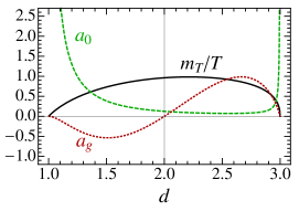
Figure 2: Thermal mass $m_{T}/T=\Theta_{d}$, as well as expansion coefficients $a_{0},a_{g}$ appearing in $\chi_{s}(|k|\gg T)$ as a function of the spatial dimension $d$. Interestingly, $a_{g}$ vanishes in $2+1$D.

Eq. (28) then leads to an asymptotic expansion of $\chi_{s}^{\rm E}$:

$$\chi_{s}^{\rm E}(k)=-\frac{N}{a_{0}}|k|^{4-D}\left(1-a_{g}\frac{T^{2}}{|k|^{2}}+a_{T}\frac{T^{D}}{|k|^{D}}+\dotsb\right)\,,$$ (32)

where we have reinstated the the full dependence on $|k|^{2}=\omega_{n}^{2}+{\bf k}^{2}$. In two spatial dimensions the above simplifies to:

$$\chi_{s}^{\rm E}(k)=-8N|k|^{3}\left(1+\frac{2^{8}\zeta(3)}{5\pi}\frac{T^{3}}{|k|^{3}}+\dotsb\right)\,.$$ (33)

Interestingly, from Eq. (30) we note that $a_{g}$ vanishes exactly in $d=2$ spatial dimensions (but not when $d\neq 2$). This stems from the fact that the OPE coefficient of $\mathcal{O}_{\!g}$ in the $\mathcal{O}_{\!g}\mathcal{O}_{\!g}$ OPE, $\mathcal{C}_{ggg}$, vanishes exactly in $d=2$ and $N=\infty$. This was previously noted in Ref. Petkou and Vlachos, 1998, where the expansion Eq. (32) was also given. As mentioned in the main body, we do not expect that $\mathcal{C}_{ggg}$ vanishes at finite $N$. In agreement with this expectation, the OPE coefficient in the Ising case ($N\!=\!1)$ was recently computedCaselle et al. (2015) by means of Monte Carlo simulations and found to be finite. It would be interesting to compare this new result with conformal bootstrap or with a $1/N$ expansion on the field theory side.

B.2 Thermal mass

Interestingly, by imposing the vanishing of forbidden terms in the asymptotics of a 2-point function such as $\chi_{s}$, we can determine the value of the thermal mass, $m_{T}=\Theta_{d}T$. Indeed, reverting back to the integration variable ${\bf k}$ in Eq. (28), we find that setting $[\cdots]=0$ leads to the following integral equation for $\Theta_{d}$:

$$-\Theta_{d}T^{d-1}X_{d+1}+\int\frac{{\rm d}^{d}{\bf k}}{(2\pi)^{d}}\frac{n_{B}(\epsilon_{k})}{\epsilon_{k}}=0\,,$$ (34)

where $\epsilon_{k}=\sqrt{{\bf k}^{2}+(\Theta_{d}T)^{2}}$, and we introduced the dimensionless constant $X_{d+1}=2\Gamma((3-d)/2)/[(4\pi)^{(d+1)/2}(d-1)]$. This agrees exactly with the equation obtained by requiring that $\varphi_{a}\varphi_{a}=1$ in the non-linear sigma modelChubukov et al. (1994); Sachdev (2011). In $D=3$, this equation can be exactly solvedChubukov et al. (1994): $\Theta_{d}=2\ln\varphi$, where $\varphi=(1+\sqrt{5})/2$ is the golden ratio.

B.3 Response function and sum rule

The scalar response function is defined as follows:

$$\mathcal{R}_{s}(\omega,{\bf k})=\frac{\chi_{s}^{R}(\omega,{\bf k})}{i\omega-0^{+}}\,,$$ (35)

where $\chi_{s}$ is the susceptibility. We shall set the spatial momentum ${\bf k}$ to zero for simplicity. Our goal is to explicitly verify the sum rule for $\mathcal{R}_{s}$. Using the general result given in the main text, Eq. (6), we have at $N=\infty$:

$$\int_{0}^{\infty}{\rm d}\omega\operatorname{Re}\left[\mathcal{R}_{s}(\omega)-\mathcal{R}_{s}^{T=0}(\omega)\right]=0\,,$$ (36)

which is precisely Eq. (10). Using the asymptotics obtained above, we find that $\mathcal{R}_{s}^{T=0}(\omega)=(N/a_{0})(\omega/i)^{3-D}$, which becomes frequency independent for $D=3$. After subtracting this leading asymptotic behavior, the integrand decays sufficiently fast for the sum rule to be well-defined. Indeed, using Eq. (32), we have for $\omega\gg T$:

$$\mathcal{R}_{s}(\omega)-\mathcal{R}_{s}^{T=0}(\omega)=-\frac{(a_{g}N/a_{0})T^{2}}{(-i\omega)^{D-1}}+\dotsb\,,$$ (37)

which comes from the relevant scalar $\mathcal{O}_{\!g}$, with scaling dimension $\Delta_{g}^{N=\infty}=2$ for $2<D<4$.

We now provide some details regarding the numerical verification of the sum rule. In general, the real part of the response is given by:

$$\operatorname{Re}\mathcal{R}_{s}(\omega)=-\pi\chi_{s}^{R}(0)\delta(\omega)+\frac{1}{\omega}\operatorname{Im}\chi_{s}^{R}(\omega)\,.$$ (38)

At $N=\infty$, we haveChubukov et al. (1994); Sachdev (2011) $\chi_{s}^{R}(\omega)=-N/\Pi^{R}(\omega)$, so that the spectral function for $\chi_{s}^{R}$ becomes

$$\operatorname{Im}\chi_{s}^{R}(\omega)=N\frac{\operatorname{Im}\Pi^{R}(\omega)}{\left|\Pi^{R}(\omega)\right|^{2}}\,,$$ (39)

where $|\Pi^{R}(\omega)|$ is the complex norm. The imaginary and real parts of $\Pi^{R}(\omega)$ at $\omega>0$ can be obtained from Eq. (27):

$$\operatorname{Im}\Pi^{R}(\omega) =\Theta(\omega-2m_{T})\frac{\pi K_{d}}{4\omega}\left[(\omega/2)^{2}-m_{T}^{2}\right]^{(d-2)/2}[1+2n_{B}(\omega/2)]\,;$$ (40)

$$\operatorname{Re}\Pi^{R}(\omega) =K_{d}\,\mathcal{P}\!\!\int_{m_{T}}^{\infty}{\rm d}\epsilon(\epsilon^{2}-m_{T}^{2})^{(d-2)/2}\frac{1+2n_{B}(\epsilon)}{4\epsilon^{2}-\omega^{2}}\,,$$ (41)

where $\Theta(x)$ is the step function, and $\mathcal{P}\!\!\int$ denotes the integral’s principal value. We note that $\operatorname{Im}\chi_{s}^{R}(\omega)$ and $\operatorname{Re}\mathcal{R}_{s}(\omega)$ vanish for $0<\omega<2m_{T}$, where $m_{T}$ is the “thermal mass” of the quasiparticles at $N=\infty$, Eq. (25). This hard gap behavior is an artefact of the $N=\infty$ limit. We further note that $\operatorname{Re}\Pi^{R}$ has a logarithmic divergence at the threshold $\omega=2m_{T}$. The resulting numerical plots for $\operatorname{Re}\mathcal{R}_{s}(\omega)$ are given in Fig. 3a. Ref. Witczak-Krempa et al., 2012 has computed $\operatorname{Im}\chi_{s}(\omega,{\bf k})$ at frequency and momentum ${\bf k}$, where additional subtleties in the integrals emerge. The calculations of Ref. Witczak-Krempa et al., 2012 can be used to verify the momentum-dependent sum rules, a task we leave for future investigation. We finally note that $\operatorname{Re}\mathcal{R}_{s}$ has a delta function at $\omega=0$, Eq. (38), the weight of which is given by

$$-\pi\chi_{s}^{R}(0)=\frac{N\pi}{\Pi^{R}(0)}\,,$$ (42)

which is plotted in Fig. 3b as a function of $D$. For $D=3$, we obtain $N\times 53.04194$.

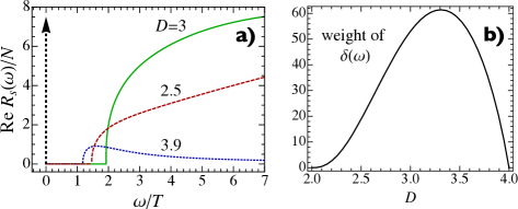
Figure 3: a) Scalar response of the O$(N)$ model ($N=\infty$) in various spacetime dimensions $D$. The dashed vertical arrow represents a delta function $\delta(\omega)$. b) Weight of this delta function versus $D$.

The integral for the sum rule Eq. (36) can be divided into three parts: the $\omega=0$ delta function, the interval $(0,2m_{T})$ where $\operatorname{Re}\mathcal{R}_{s}$ vanishes, and $(2m_{T},+\infty)$:

$$\mathcal{I}=-\frac{\pi}{2}\chi_{s}^{R}(0)+\int_{0}^{2m_{T}}\!\!{\rm d}\omega\operatorname{Re}\left[0-\mathcal{R}_{s}^{T=0}(\omega)\right]+\int_{2m_{T}}^{\infty}\!\!{\rm d}\omega\operatorname{Re}\left[\mathcal{R}_{s}(\omega)-\mathcal{R}_{s}^{T=0}(\omega)\right]\,.$$ (43)

For $D=3$, we numerically find:

$$-\frac{\pi}{2}\chi_{s}^{R}(0) =+26.520972\,;$$

$$-\int_{0}^{2m_{T}}\!\!{\rm d}\omega\operatorname{Re}\mathcal{R}_{s}^{T=0}(\omega) =-15.398778\,;$$

$$\int_{2m_{T}}^{\infty}\!\!{\rm d}\omega\operatorname{Re}\left[\mathcal{R}_{s}(\omega)-\mathcal{R}_{s}^{T=0}(\omega)\right] =-11.122193\,.$$ (44)

The terms sum to $\mathcal{I}=1.9\times 10^{-7}$. We can attribute the deviation from zero to the numerical uncertainty in our evaluation of the integrals. (We emphasize that care must be used to treat the logarithmic vanishing of $\operatorname{Re}\mathcal{R}_{s}$ at the threshold $\omega=2m_{T}$.) The fact that three numbers of order $10^{1}$ cancel to within $10^{-7}$ provides an excellent check of the sum rule. We have also verified the sum rule for other spacetime dimensions $D$, and have found that it is respected, in accordance with the proof given in the main body.

References

- Pelissetto and Vicari (2002) A. Pelissetto and E. Vicari, Physics Reports 368, 549 (2002), cond-mat/0012164 .
- Zinn-Justin (2002) J. Zinn-Justin, Int.Ser.Monogr.Phys. 113, 1 (2002).
- Sachdev (2011) S. Sachdev, Quantum Phase Transitions, 2nd ed. (Cambridge University Press, England, 2011).
- El-Showk et al. (2012) S. El-Showk, M. F. Paulos, D. Poland, S. Rychkov, D. Simmons-Duffin, and A. Vichi, Phys. Rev. D 86, 025022 (2012), arXiv:1203.6064 [hep-th] .
- Chubukov et al. (1994) A. V. Chubukov, S. Sachdev, and J. Ye, Phys. Rev. B 49, 11919 (1994), arXiv:cond-mat/9304046 .
- Katz et al. (2014) E. Katz, S. Sachdev, E. S. Sørensen, and W. Witczak-Krempa, Phys. Rev. B 90, 245109 (2014), arXiv:1409.3841 [cond-mat.str-el] .
- Wilson (1969) K. G. Wilson, Phys. Rev. 179, 1499 (1969).
- Ferrara et al. (1972) S. Ferrara, A. F. Grillo, and R. Gatto, Phys. Rev. D 5, 3102 (1972).
- Polyakov (1974) A. Polyakov, Zh.Eksp.Teor.Fiz. 66, 23 (1974).
- Note (1) We stay away from the lightcone .
- Caron-Huot (2009) S. Caron-Huot, Phys.Rev. D79, 125009 (2009), arXiv:0903.3958 [hep-ph] .
- Mack (1977) G. Mack, Comm. Math. Phys. 55, 1 (1977).
- (13) J. Maldacena, Private communication.
- Gulotta et al. (2011) D. R. Gulotta, C. P. Herzog, and M. Kaminski, JHEP 1101, 148 (2011), arXiv:1010.4806 [hep-th] .
- Witczak-Krempa and Sachdev (2012) W. Witczak-Krempa and S. Sachdev, Phys.Rev. B86, 235115 (2012), arXiv:1210.4166 [cond-mat.str-el] .
- Witczak-Krempa and Sachdev (2013) W. Witczak-Krempa and S. Sachdev, Phys. Rev. B 87, 155149 (2013), arXiv:1302.0847 [cond-mat.str-el] .
- Witczak-Krempa (2014) W. Witczak-Krempa, Phys. Rev. B 89, 161114 (2014), arXiv:1312.3334 [cond-mat.str-el] .
- pol (1987) Gauge Fields and Strings, Contemporary concepts in physics (Taylor & Francis, 1987).
- Kos et al. (2014) F. Kos, D. Poland, and D. Simmons-Duffin, Journal of High Energy Physics 6, 91 (2014), arXiv:1307.6856 [hep-th] .
- El-Showk et al. (2014a) S. El-Showk, M. Paulos, D. Poland, S. Rychkov, D. Simmons-Duffin, and A. Vichi, Physical Review Letters 112, 141601 (2014a), arXiv:1309.5089 [hep-th] .
- El-Showk et al. (2014b) S. El-Showk, M. F. Paulos, D. Poland, S. Rychkov, D. Simmons-Duffin, and A. Vichi, Journal of Statistical Physics (2014b), 10.1007/s10955-014-1042-7, arXiv:1403.4545 [hep-th] .
- Caselle et al. (2015) M. Caselle, G. Costagliola, and N. Magnoli, ArXiv e-prints (2015), arXiv:1501.04065 [hep-th] .
- Petkou and Vlachos (1998) A. C. Petkou and N. D. Vlachos, ArXiv High Energy Physics - Theory e-prints (1998), hep-th/9809096 .
- Endres et al. (2012) M. Endres, T. Fukuhara, D. Pekker, M. Cheneau, P. Schau, C. Gross, E. Demler, S. Kuhr, and I. Bloch, Nature (London) 487, 454 (2012), arXiv:1204.5183 [cond-mat.quant-gas] .
- Pollet and Prokof’ev (2012) L. Pollet and N. Prokof’ev, Physical Review Letters 109, 010401 (2012), arXiv:1204.5190 [cond-mat.quant-gas] .
- Podolsky and Sachdev (2012) D. Podolsky and S. Sachdev, Phys. Rev. B 86, 054508 (2012), arXiv:1205.2700 [cond-mat.quant-gas] .
- Gazit et al. (2013) S. Gazit, D. Podolsky, A. Auerbach, and D. P. Arovas, Phys. Rev. B 88, 235108 (2013), arXiv:1309.1765 [cond-mat.str-el] .
- Rançon and Dupuis (2014) A. Rançon and N. Dupuis, Phys. Rev. B 89, 180501 (2014), arXiv:1402.3098 [cond-mat.quant-gas] .
- Tenenbaum Katan and Podolsky (2014) Y. Tenenbaum Katan and D. Podolsky, ArXiv e-prints (2014), arXiv:1412.4546 [cond-mat.str-el] .
- Romatschke and Son (2009) P. Romatschke and D. T. Son, Phys. Rev. D 80, 065021 (2009), arXiv:0903.3946 [hep-ph] .
- Taylor and Randeria (2010) E. Taylor and M. Randeria, Phys. Rev. A 81, 053610 (2010).
- Enss et al. (2011) T. Enss, R. Haussmann, and W. Zwerger, Annals of Physics 326, 770 (2011), arXiv:1008.0007 [cond-mat.quant-gas] .
- Goldberger and Khandker (2012) W. D. Goldberger and Z. U. Khandker, Phys. Rev. A 85, 013624 (2012), arXiv:1107.1472 [cond-mat.quant-gas] .
- Šmakov and Sørensen (2005) J. Šmakov and E. S. Sørensen, Physical Review Letters 95, 180603 (2005), arXiv:cond-mat/0509671 .
- Witczak-Krempa et al. (2014) W. Witczak-Krempa, E. S. Sørensen, and S. Sachdev, Nature Physics 10, 361 (2014), arXiv:1309.2941 [cond-mat.str-el] .
- Chen et al. (2014) K. Chen, L. Liu, Y. Deng, L. Pollet, and N. Prokof’ev, Phys. Rev. Lett. 112, 030402 (2014).
- Swanson et al. (2014) M. Swanson, Y. L. Loh, M. Randeria, and N. Trivedi, Physical Review X 4, 021007 (2014), arXiv:1310.1073 [cond-mat.supr-con] .
- Gazit et al. (2014) S. Gazit, D. Podolsky, and A. Auerbach, Physical Review Letters 113, 240601 (2014), arXiv:1407.1055 [cond-mat.str-el] .
- Maldacena (1998) J. M. Maldacena, Adv.Theor.Math.Phys. 2, 231 (1998), arXiv:hep-th/9711200 [hep-th] .
- Witczak-Krempa et al. (2012) W. Witczak-Krempa, P. Ghaemi, T. Senthil, and Y. B. Kim, Phys. Rev. B 86, 245102 (2012), arXiv:1206.3309 [cond-mat.str-el] .