Stability of Markov regenerative switched linear systems

Abstract

In this paper, we give a necessary and sufficient condition for mean stability of switched linear systems having a Markov regenerative process as its switching signal. This class of switched linear systems, which we call Markov regenerative switched linear systems, contains Markov jump linear systems and semi-Markov jump linear systems as special cases. We show that a Markov regenerative switched linear system is $m$th mean stable if and only if a particular matrix is Schur stable, under the assumption that either $m$ is even or the system is positive.

,

1 Introduction

Among switched linear systems, those having a time-homogeneous Markov process as its switching signal, called Markov jump linear systems [Costa2013], are of particular importance. One of the reasons for their importance is that time-homogeneous Markov processes are well suited to model stochastic phenomena presenting a constant rate of occurrence. Another reason is that the analysis and synthesis of Markov jump linear systems can be performed in a rather similar way to those for linear time-invariant systems by the introduction of auxiliary variables [Costa2013].

However, it is often restricting to assume that the switching signals present constant transition rates, or even the Markovian property. To overcome this restriction, we find a wide variety of alternative switching signals in the literature [Hou2005, Antunes2013, Ogura2014d, Ogura2013f]. A natural extension to time-homogeneous Markov processes are time-homogeneous semi-Markov processes, which are Markovian-like processes with time-varying transition rates Cinlar1975see. The stability analysis of the corresponding switched linear systems can be found in Antunes2013 and Ogura2013f. Another extension are regenerative processes [Smith1955], which are, roughly speaking, stochastic processes that can be obtained by concatenating independent and identically distributed random functions (see Sigman1993 for the details). The mean stability analysis of linear systems subject to regenerative switchings is performed in Ogura2014d.

In this paper, we extend the works in Antunes2013, Ogura2014d, and Ogura2013f to analyze the stability of Markov regenerative switched linear systems, which are switched linear systems whose switching signal is a Markov regenerative process (also called a semi-regenerative process) [Cinlar1975, Choi1994]. Markov regenerative processes form a large class of stochastic processes which contains as special cases all the Markov, semi-Markov, and regenerative processes. We show that exponential $m$th mean stability of a Markov regenerative switched linear system is characterized by the spectral radius of a matrix, under the assumption that either $m$ is even or the system is positive. Extending various results in the literature [Antunes2013, Ogura2014d, Ogura2013f, Fang2002c], the obtained result enables us to analyze the stability of, for example, state-feedbacked Markov jump linear systems with periodically observed mode signals (see a discrete-time setting in Cetinkaya2014b), as well as controlled system with failure-prone controllers with only one repairing facility [Distefano2013, Section 3.2].

The paper is organized as follows. After introducing necessary notations, in Section 2 we introduce the class of Markov regenerative switched linear systems under consideration and then state a necessary and sufficient condition for their exponential mean stability. Then, in Section 3, we present various applications of the main result. The notation used in this paper is standard. When $x\in\mathbb{R}^{n}$ is nonnegative entrywise we write $x\geq 0$. The standard Euclidean norm on $\mathbb{R}^{n}$ is denoted by $\lVert\cdot\rVert$. Let $I$ and $O$ denote the identity and zero matrices, respectively. The block diagonal matrix with block diagonals $A_{1}$, $\dotsc$, $A_{N}$ is denoted by $\bigoplus_{i=1}^{N}A_{i}$. The kronecker product of two matrices $A$ and $B$ is denoted by $A\otimes B$. We say that $A\in\mathbb{R}^{n\times n}$ is Schur stable if $A$ has the spectral radius less than one. Also we say that $A$ is Hurwitz stable if all the eigenvalues of $A$ have negative real parts. For an integrable random variable $X$, its expected value is denoted by $E[X]$ and its conditional expectations by $E[X\mid\cdot]$.

2 Stability characterization

This section introduces the class of Markov regenerative switched linear systems and then presents a necessary and sufficient condition for their stability. We need to first recall the definition of Markov renewal processes [Cinlar1975]. Let $N$ be a positive integer. A stochastic process $(\theta,\tau)=\{(\theta_{k},\tau_{k})\}_{k\geq 0}$ taking values in $\{1,\dotsc,N\}\times[0,\infty)$ and satisfying $0=\tau_{0}\leq\tau_{1}\leq\cdots$ is called a Markov renewal process [Cinlar1975] if

$$\begin{multlined}P(\theta_{k+1}=j,\tau_{k+1}-\tau_{k}\leq t\mid\theta_{k},\dotsc,\theta_{0},\tau_{k},\dotsc,\tau_{0})\\ =P(\theta_{k+1}=j,\tau_{k+1}-\tau_{k}\leq t\mid\theta_{k})\end{multlined}P(\theta_{k+1}=j,\tau_{k+1}-\tau_{k}\leq t\mid\theta_{k},\dotsc,\theta_{0},\tau_{k},\dotsc,\tau_{0})\\ =P(\theta_{k+1}=j,\tau_{k+1}-\tau_{k}\leq t\mid\theta_{k})$$

holds for every $k$ and $t\geq 0$. We assume that $(\theta,\tau)$ is time-homogeneous, that is, for all $i,j$ and $t\geq 0$, the probability $P(\theta_{k+1}=j,\tau_{k+1}-\tau_{k}\leq t\mid\theta_{k}=i)$ is independent of $k$. We note that, in this case, $\theta$ is a time-homogeneous Markov chain and therefore has the constant transition probabilities $P(\theta_{k+1}=j\mid\theta_{k}=i)$. In this paper, we furthermore assume that

$$\tau_{k+1}-\tau_{k}>0$$ (1)

with probability one for every $k$. Then, we can state the definition of Markov regenerative processes as follows.

Definition 1 (Cinlar1975, Choi1994).

Let $\sigma=\{\sigma_{t}\}_{t\geq 0}$ be a stochastic process taking values in a finite set $\Lambda$. We say that $\sigma$ is Markov regenerative if there exists a Markov renewal process $(\theta,\tau)$ taking values in $\{1,\dotsc,N\}\times[0,\infty)$ and satisfying the following conditions for every $k$:

1. $\tau_{k}$ is a stopping time for $\sigma$;

2. There exists a function $\pi\colon\Lambda\to\{1,\dotsc,N\}$ such that $\pi(\sigma_{\tau_{k}})=\theta_{k}$;

3. For $j\in\{1,\dotsc,N\}$, $\ell\geq 1$, $0\leq t_{1}<t_{2}<\cdots<t_{\ell}$, and a function $f\colon\Lambda^{\ell}\to[0,\infty)$,

   $$\begin{multlined}E[f(\sigma_{\tau_{k}+t_{1}},\dotsc,\sigma_{\tau_{k}+t_{\ell}})\mid\theta_{k}=j,\sigma_{s};s\leq\tau_{k}]\\ =E[f(\sigma_{t_{1}},\dotsc,\sigma_{t_{\ell}})\mid\theta_{0}=j].\end{multlined}E[f(\sigma_{\tau_{k}+t_{1}},\dotsc,\sigma_{\tau_{k}+t_{\ell}})\mid\theta_{k}=j,\sigma_{s};s\leq\tau_{k}]\\ =E[f(\sigma_{t_{1}},\dotsc,\sigma_{t_{\ell}})\mid\theta_{0}=j].$$

We call $\tau$ the regeneration times of $\sigma$, and $(\theta,\tau)$ the embedded Markov renewal process of $\sigma$.

Among the three conditions in the definition, (P3) is the most important. It implies that, as far as prediction is concerned, at the regeneration time $\tau_{k}$, the past information of the process $\{\sigma_{s}\}_{s\leq\tau_{k}}$ is irrelevant and only the value of $\theta_{k}$ is needed. Actually, (P3) implies that

$$P(\sigma_{\tau_{k}+t}=\lambda\mid\theta_{k}=j,\sigma_{s};s\leq\tau_{k})=P(\sigma_{t}=\lambda\mid\theta_{0}=j)$$ (2)

for all $\lambda\in\Lambda$, $i,j\in\{1,\dotsc,N\}$, $t\geq 0$, and $k\geq 0$. Equation (2) indicates that, given $\theta_{k}=j$, the process $\sigma$ “regenerates” at time $\tau_{k}$ as if it starts from time $0$, given $\theta_{0}=j$. Moreover, $\sigma$ possesses a certain Markovian property at the regeneration time $\tau_{k}$; once we know the value of $\sigma_{\tau_{k}}$, using (P2) we can determine the value $\theta_{k}$, which then determines the future distribution of $\sigma$ by (2). As is pointed out in Cinlar1974, it is convenient to take $\pi$ to be the identity, but this is not necessary. Also we remark that (P1) is a technical condition needed to state (P3). For the details, the readers are referred to Cinlar1975 and Cinlar1974.

Then, we introduce the class of switched linear systems studied in this paper.

Definition 2.

Let $\sigma$ be a Markov regenerative process and let $A_{\lambda}\in\mathbb{R}^{n\times n}$ for each $\lambda\in\Lambda$. Then, the stochastic differential equation

$$\Sigma:\frac{dx}{dt}=A_{\sigma_{t}}x,$$ (3)

where $x(0)=x_{0}\in\mathbb{R}^{n}$ is a constant, is called a Markov regenerative switched linear system.

For example, a time-homogeneous Markov process $r$ is Markov regenerative with an underlying embedded Markov renewal process being $\{(r_{t_{k}},t_{k})\}_{k\geq 0}$, where $0=t_{0}<t_{1}<t_{2}<\cdots$ are the times at which the process $r$ changes its value. Therefore, Markov jump linear systems [Costa2013] are Markov regenerative switched linear systems. In Section 3, we will show in detail that more general classes of switched linear systems, such as semi-Markov jump linear systems [Antunes2013, Ogura2013f] and regenerative switched linear systems [Ogura2014d], are contained in the class of Markov regenerative switched linear systems.

Based on the embedded Markov renewal process, we can naturally define the stability of Markov regenerative switched linear systems as follows.

Definition 3.

Given a positive integer $m$, we say that $\Sigma$ is exponentially $m$th mean stable if there exist $C>0$ and $\beta>0$ such that $E[\lVert x(t)\rVert^{m}]\leq Ce^{-\beta t}\lVert x_{0}\rVert^{m}$ for every $x_{0}$ and $\theta_{0}$.

Also, we here introduce the positivity of $\Sigma$.

Definition 4.

We say that $\Sigma$ is positive if $x_{0}\geq 0$ implies $x(t)\geq 0$ with probability one for all $\theta_{0}$ and $t\geq 0$.

We remark that, for $\Sigma$ to be positive, it is clearly sufficient that all the matrices $A_{\lambda}$ ($\lambda\in\Lambda$) are Metzler, i.e., the off-diagonal entries of each $A_{\lambda}$ are all nonnegative [Farina2000]. However, this sufficient condition is not necessary as is shown in [Example 10]Ogura2014d for regenerative switched linear systems.

In order to state the main result of this paper, we recall the notion of induced matrices. First we define Parrilo2008see, e.g., the $m$-lift of $x\in\mathbb{R}^{n}$, denoted by $x^{[m]}$, as the real vector of length $n_{m}=\binom{n+m-1}{m}$ with its elements being the lexicographically ordered monomials $\sqrt{\alpha!}\,x^{\alpha}$ ($\alpha!:={m!}/(\alpha_{1}!\dotsm\alpha_{n}!)$) that are indexed by all the possible exponents $\alpha=(\alpha_{1},\dotsc,\alpha_{n})$ summing up to $m$. For example, for $x=[x_{1},x_{2}]^{\top}$ we have $x^{[1]}=x$, $x^{[2]}=[x_{1}^{2},\sqrt{2}x_{1}x_{2},x_{2}^{2}]^{\top}$, and $x^{[3]}=[x_{1}^{3},\sqrt{3}x_{1}^{2}x_{2},\sqrt{3}x_{1}x_{2}^{2},x_{2}^{3}]^{\top}$. Then, we define the $m$th induced matrix of $A$, denoted by $A^{[m]}$, as the $n_{m}\times n_{m}$ unique matrix [Parrilo2008] satisfying $(Ax)^{[m]}=A^{[m]}x^{[m]}$ for every $x\in\mathbb{R}^{n}$.

The next theorem is the main result of this paper.

Theorem 5.

Let $p_{ij}=P(\theta_{1}=j\mid\theta_{0}=i)$ for all $i,j\in\{1,\dotsc,N\}$. For all $0\leq s\leq t<\infty$, define the $\mathbb{R}^{n\times n}$-valued random variable $\Phi(t;s)$ by the differential equation ${\partial\Phi}/{\partial t}=A_{\sigma_{t}}\Phi(t;s)$ with the initial conditions $\Phi(t;t)=I_{n}$ for every $t\geq 0$. Assume that the following two conditions hold:

1. Either $m$ is even or $\Sigma$ is positive;

2. There exists $T>0$ such that $\tau_{k+1}-\tau_{k}\leq T$ with probability one for every $k\geq 0$.

Then, $\Sigma$ is exponentially $m$th mean stable if and only if the $(Nn_{m})\times(Nn_{m})$ real block matrix $\mathcal{A}=[\mathcal{A}_{ij}]_{1\leq i,j\leq N}$ with the $(i,j)$-block $\mathcal{A}_{ij}$ being defined by

$$\mathcal{A}_{ij}=p_{ji}E[\Phi(\tau_{1};0)^{[m]}\mid\theta_{0}=j,\theta_{1}=i]$$ (4)

is Schur stable.

In Section 3, we will show that the above theorem can recover stability characterizations of Markov jump linear systems [Fang2002c, Ogura2013f], semi-Markov jump linear systems [Antunes2013, Ogura2013f], and regenerative switched linear systems [Ogura2014d]. We will also show that the theorem can give a stability condition for other switched linear systems whose stability cannot be studied using the methods in the literature.

2.1 Proof

We present a proof of Theorem 5 in this subsection. This proof consists of the following two steps. We first show, in Proposition 6, that the stability of $\Sigma$ can be analyzed based on its discretized version. The proof of the proposition utilizes the technique developed in Ogura2014d to study regenerative switched linear systems. To analyze the discretized version of the system, we then present Proposition 7, which extends Theorem 3.4 in Ogura2013f for not necessarily positive systems.

Let $\Sigma$ be a Markov regenerative switched linear system. Then, the discretized process $x_{d}=\{x(\tau_{k})\}_{k\geq 0}$ is the solution of the discrete-time system $\mathcal{S}\Sigma:x_{d}(k+1)=\Phi(\tau_{k+1};\tau_{k})x_{d}(k)$. In order to proceed, we introduce a class of switched linear systems called discrete-time semi-Markov jump linear systems [Ogura2013f]. Let $\{F_{k}\}_{k\geq 0}$ be a stochastic process taking values in $\mathbb{R}^{n\times n}$. The system $\Sigma_{d}:x_{d}(k+1)=F_{k}x_{d}(k)$ ($x_{d}(0)=x_{0}$) is said to be a discrete-time semi-Markov jump linear system if there exists a time-homogeneous Markov chain $\theta$ taking values in $\{1,\dotsc,N\}$ such that, for all $k\geq 0$, $i,j\in\{1,\dotsc,N\}$, and a Borel subset $G$ of $\mathbb{R}^{n\times n}$, there holds that

$$\begin{multlined}P(\theta_{k+1}=j,F_{k}\in G\mid\theta_{k},\dotsc,\theta_{0},F_{k-1},\dotsc,F_{0})\\ =P(\theta_{k+1}=j,F_{k}\in G\mid\theta_{k}),\end{multlined}P(\theta_{k+1}=j,F_{k}\in G\mid\theta_{k},\dotsc,\theta_{0},F_{k-1},\dotsc,F_{0})\\ =P(\theta_{k+1}=j,F_{k}\in G\mid\theta_{k}),$$ (5)

and the conditional probability

$$P(\theta_{k+1}=j,F_{k}\in G\mid\theta_{k}=i)$$ (6)

does not depend on $k$. The mean stability and the positivity of $\Sigma_{d}$ is defined in the following standard manner. For a positive integer $m$, we say that $\Sigma_{d}$ is exponentially $m$th mean stable if there exist $C>0$ and $\beta>0$ such that $E[\lVert x_{d}(k)\rVert^{m}]\leq Ce^{-\beta k}\lVert x_{0}\rVert^{m}$ for all $x_{0}$ and $\theta_{0}$. Also we say that $\Sigma_{d}$ is stochastically $m$th mean stable if $\sum_{k=0}^{\infty}E[\lVert x_{d}(k)\rVert^{m}]$ is finite for all $x_{0}$ and $\theta_{0}$. Finally, $\Sigma_{d}$ is said to be positive if $x_{0}\geq 0$ implies $x_{d}(k)\geq 0$ with probability one for every $k$ and $\theta_{0}$.

The next proposition relates the stability of $\Sigma$ and $\mathcal{S}\Sigma$.

Proposition 6.

$\mathcal{S}\Sigma$ is a discrete-time semi-Markov jump linear system. Moreover, if (A2) holds, then the following statements are true:

• If $\Sigma$ is exponentially $m$th mean stable, then $\mathcal{S}\Sigma$ is stochastically $m$th mean stable.

• If $\mathcal{S}\Sigma$ is exponentially $m$th mean stable, then so is $\Sigma$.

Let $F_{k}=\Phi(\tau_{k+1};\tau_{k})$. Also, we let $(\Omega,\mathcal{M},P)$ denote the underlying probability space. We denote the $\sigma$-algebra of $\Omega$ generated by a set $X$ of random variables by $\mathcal{M}(X)$. We define the following $\sigma$-algebras; $\mathcal{M}_{1}=\mathcal{M}(\{\theta_{k}\})$, $\mathcal{M}_{2}=\mathcal{M}(\{\theta_{k},\dotsc,\theta_{0},F_{k-1},\dotsc,F_{0}\})$, $\mathcal{M}_{3}=\mathcal{M}(\{\theta_{k},\dotsc,\theta_{0},\sigma_{s};{s\leq\tau_{k}}\})$, and $\mathcal{M}_{4}=\mathcal{M}(\{\theta_{k},\sigma_{s};s\leq\tau_{k}\})$. Then, we can show

$$\mathcal{M}_{1}\subset\mathcal{M}_{2}\subset\mathcal{M}_{3}=\mathcal{M}_{4}.$$ (7)

The first inclusion is obvious. The second inclusion is true because $F_{0},\dotsc,F_{k-1}$ are measurable on $\mathcal{M}_{3}$. Finally, the last identity follows from (P2). Now, from (P3) we know that $P(\theta_{k+1}=j,F_{k}\in G\mid\mathcal{M}_{1})=P(\theta_{k+1}=j,F_{k}\in G\mid\mathcal{M}_{4})$. Therefore, by (7) and [Lemma 1.1]Ogura2013f, we conclude that $P(\theta_{k+1}=j,F_{k}\in G\mid\mathcal{M}_{1})=P(\theta_{k+1}=j,F_{k}\in G\mid\mathcal{M}_{2})$, which is equivalent to (5). Also, the conditional probability (6) is independent of $k$ by (P3) and the time-homogeneity of $\theta$. Therefore, $\mathcal{S}\Sigma$ is a discrete-time semi-Markov jump linear system.

The proof of the second statement can be done in the same way as the proof for the implication $[2\Rightarrow 3]$ of [Theorem 12]Ogura2014d due to (A2) and the assumption (1). Also, we can prove the third statement in the same way as the proof for $[3\Rightarrow 1]$ of [Theorem 12]Ogura2014d by (A2). The details of the proofs are thus omitted.

Proposition 6 shows that the stability analysis of $\Sigma$ could be reduced to the stability analysis of discrete-time semi-Markov jump linear systems. The next proposition gives a characterization of the exponential $m$th mean stability of discrete-time semi-Markov jump linear systems, extending [Theorem 3.4]Ogura2013f to the case where $m$ is even.

Proposition 7.

For $i,j\in\{1,\dotsc,N\}$, let $p_{ij}$ denote the transition probability of $\theta$ from $i$ to $j$. Assume that either $m$ is even or $\Sigma_{d}$ is positive. Then, the following statements are equivalent.

1. $\Sigma_{d}$ is exponentially $m$th mean stable;

2. $\Sigma_{d}$ is stochastically $m$th mean stable;

3. The $(Nn_{m})\times(Nn_{m})$ block matrix $\mathcal{F}$ with the $(i,j)$-block $\mathcal{F}_{ij}=p_{ji}E[F_{0}^{[m]}\mid\theta_{0}=j,\theta_{1}=i]\in\mathbb{R}^{n_{m}\times n_{m}}$ is Schur stable.

For the proof of this proposition, we will need the next lemma.

Lemma 8.

Assume that $m$ is an even integer. Let $K$ be the closed convex hull of $(\mathbb{R}^{n})^{[m]}=\{x^{[m]}:x\in\mathbb{R}^{n}\}$ in $\mathbb{R}^{n_{m}}$. Then, there exists a norm ${|\kern-1.07639pt|\kern-1.07639pt|\cdot|\kern-1.07639pt|\kern-1.07639pt|}$ on $\mathbb{R}^{Nn_{m}}$ and $f\in\mathbb{R}^{Nn_{m}}$ such that ${|\kern-1.07639pt|\kern-1.07639pt|x|\kern-1.07639pt|\kern-1.07639pt|}=f^{\top}x$ for every $x\in K\times\cdots\times K$.

We first show that $K$ is a proper cone [Tam2006, Chapter 26], that is, $K$ is a closed and convex cone having a nonempty interior and satisfying

$$K\cap(-K)=\{0\},$$ (8)

where $-K:=\{-x:x\in K\}$. $K$ is clearly a closed and convex cone.

Let us show (8). For each $i\in\{1,\dotsc,n\}$, let $\ell_{i}$ denote the position of the monomial $x_{i}^{m}$ in the vector $x^{[m]}$, i.e., we assume that $(x^{[m]})_{\ell_{i}}=x_{i}^{m}$. Let us show the existence of a constant $C>0$ such that every $y\in K$ satisfies

$$y_{\ell_{i}}\geq 0,\ \lvert y_{\ell}\rvert\leq C\sum_{i=1}^{n}y_{\ell_{i}},$$ (9)

for all $1\leq i\leq n$ and $1\leq\ell\leq n_{m}$. Take an arbitrary $y$ in the convex hull of $(\mathbb{R}^{n})^{[m]}$. Then there exist $x_{1},\dotsc,x_{N}\in\mathbb{R}^{n}$ and positive numbers $c_{1},\dotsc,c_{N}$ such that $y=\sum_{j=1}^{N}c_{j}x_{j}^{[m]}$. Without loss of generality we can assume $c_{j}=1$. Then, $y_{\ell_{i}}=\sum_{j=1}^{N}(x_{j})_{i}^{m}\geq 0$ because $m$ is even. Next, let $1\leq\ell\leq n_{m}$ be arbitrary and let $\alpha=(\alpha_{1},\dotsc,\alpha_{n})$ be the exponent of the monomial $(x^{[m]})_{\ell}$, i.e., we suppose that $(x^{[m]})_{\ell}=\sqrt{\alpha!}x^{\alpha}$. Then, the inequality of arithmetic and geometric means implies $\lvert(x^{[m]})_{\ell}\rvert\leq m^{-1}\sqrt{\alpha!}\sum_{i=1}^{n}\alpha_{i}x_{i}^{m}$. Hence, the triangle inequality shows that $\lvert y_{\ell}\rvert\leq\sum_{j=1}^{N}\lvert(x_{j}^{[m]})_{\ell}\rvert\leq m^{-1}\sqrt{\alpha!}\sum_{i=1}^{n}\sum_{j=1}^{N}(x_{j})_{i}^{m}\leq C\sum_{i=1}^{n}y_{\ell_{i}}$, where $C=m^{-1}\max_{\alpha}(\sqrt{\alpha!})$. Therefore, every $y$ in the convex hull of $(\mathbb{R}^{n})^{[m]}$ satisfies (9). A limiting argument thus shows that (9) is satisfied by every $y\in K$. Now assume $y,-y\in K$. This implies $y_{\ell_{i}}=0$ for every $i$ and therefore $y_{\ell}=0$ for every $\ell$ by (9). Hence (8) holds.

Finally, by [Lemma 1.5]Ogura2013f, the difference $K-K=\{x-y:x,y\in K\}$ equals the whole space $\mathbb{R}^{n_{m}}$. This in fact shows that the interior of $K$ is nonempty because, in general, a closed and convex cone $K$ satisfying (8) has a nonempty interior if and only if the difference $K-K$ coincides with the whole space [Tam2006, Chapter 26].

Now, since $K$ is a proper cone, the $N$-direct product $K\times\cdots\times K$ in $\mathbb{R}^{Nn_{m}}$ is also a proper cone. Therefore there exists [Seidman2005, Section 2] a norm ${|\kern-1.07639pt|\kern-1.07639pt|\cdot|\kern-1.07639pt|\kern-1.07639pt|}$ on $\mathbb{R}^{Nn_{m}}$ and a vector $f\in\mathbb{R}^{Nn_{m}}$ having the desired property. This completes the proof.

We then prove Proposition 7:

The case where $\Sigma_{d}$ is positive is shown in [Theorem 3.4]Ogura2013f. Let us assume that $m$ is even. We shall show the cycle [1 $\Rightarrow$ 2 $\Rightarrow$ 3 $\Rightarrow$ 1]. It is easy to prove [1 $\Rightarrow$ 2]. The implication [2 $\Rightarrow$ 3] can be proved in the same way as in the proof of Theorem 3.4 in Ogura2013f without the positivity assumption.

Let us prove [3 $\Rightarrow$ 1] assuming $m$ is even. Take a norm ${|\kern-1.07639pt|\kern-1.07639pt|\cdot|\kern-1.07639pt|\kern-1.07639pt|}$ on $\mathbb{R}^{Nn_{m}}$ and $f\in\mathbb{R}^{Nn_{m}}$ satisfying the linearity property described in Lemma 8. By the equivalence of the norms on a finite-dimensional linear space, we can take a constant $C_{1}>0$ such that $C_{1}^{-1}\lVert\cdot\rVert\leq{|\kern-1.07639pt|\kern-1.07639pt|\cdot|\kern-1.07639pt|\kern-1.07639pt|}\leq C_{1}\lVert\cdot\rVert$. Let us consider the stochastic process $e_{\theta_{k}}$, where $e_{1}$, $\dotsc$, $e_{N}$ denote the standard unit vectors in $\mathbb{R}^{N}$. Using the general identity $\lVert x^{[m]}\rVert=\lVert x\rVert^{m}$ Parrilo2008see, we can show the inequality $\lVert x_{d}(k)\rVert^{m}=\lVert x_{d}(k)^{[m]}\rVert=\lVert e_{\theta_{k}}\otimes x_{d}(k)^{[m]}\rVert\leq C_{1}{|\kern-1.07639pt|\kern-1.07639pt|e_{\theta_{k}}\otimes x_{d}(k)^{[m]}|\kern-1.07639pt|\kern-1.07639pt|}$. Since $e_{\theta_{k}}\otimes x_{d}(k)^{[m]}\in K\times\cdots\times K$, the linearity of the norm ${|\kern-1.07639pt|\kern-1.07639pt|\cdot|\kern-1.07639pt|\kern-1.07639pt|}$ shows that

$$E[\lVert x_{d}(k)\rVert^{m}] \leq C_{1}{|\kern-1.07639pt|\kern-1.07639pt|E[e_{\theta_{k}}\otimes x_{d}(k)^{[m]}]|\kern-1.07639pt|\kern-1.07639pt|}$$ (10)

$$\leq C_{1}^{2}\lVert E[e_{\theta_{k}}\otimes x_{d}(k)^{[m]}]\rVert.$$

On the other hand, by the identity

$$E[e_{\theta_{k+1}}\otimes x_{d}(k+1)^{[m]}]=\mathcal{F}E[e_{\theta_{k}}\otimes x_{d}(k)^{[m]}]$$ (11)

proved in [Proposition 3.8]Ogura2013f, if $\rho(\mathcal{F})<1$ then there exist $C_{2}>0$ and $\beta>0$ such that

$$\lVert E[e_{\theta_{k}}\otimes x_{d}(k)^{[m]}]\rVert \leq C_{2}e^{-\beta k}\lVert e_{\theta_{0}}\otimes x_{0}^{[m]}\rVert$$ (12)

$$=C_{2}e^{-\beta k}\lVert x_{0}^{[m]}\rVert$$

$$=C_{2}e^{-\beta k}\lVert x_{0}\rVert^{m}.$$

Therefore, the inequalities (10) and (12) prove that $\Sigma_{d}$ is exponentially $m$th mean stable. This completes the proof of Proposition 7.

Now we can readily prove Theorem 5. (A1) implies that either $m$ is even or $\mathcal{S}\Sigma$ is positive. Therefore, by Proposition 7 and the first statement of Proposition 6, we see that the following three properties are equivalent; the exponential $m$th mean stability of $\mathcal{S}\Sigma$, the stochastic $m$th mean stability of $\mathcal{S}\Sigma$, and the Schur stability of $\mathcal{A}$. This equivalence and also the second and third statements of Proposition 6 immediately prove the main result of Theorem 5.

3 Applications

In this section, we illustrate how Theorem 5, the main result of this paper, can be used to recover various stability characterizations of switched linear systems derived in the literature (Subsections 3.1–3.3), as well as to analyze the stability of systems that cannot be analyzed by current techniques in the literature (Subsection 3.4). Throughout this section, we will use the following notation Brockett1973see. For a matrix $A\in\mathbb{R}^{n\times n}$, we define $A_{[m]}\in\mathbb{R}^{n_{m}\times n_{m}}$ as the unique real matrix such that

$$(\exp(At))^{[m]}=\exp(A_{[m]}t).$$ (13)

3.1 Regenerative switched linear systems

In this subsection, we discuss some implications of the stability characterization provided for regenerative switched linear systems [Ogura2014d]. We first recall the definition of regenerative processes. We say that a stochastic process $\sigma$ is a regenerative process [Smith1955] if there exists a random variable $R_{1}>0$ such that (i) $\{\sigma_{t+R_{1}}\}_{t\geq 0}$ is independent of $\{\{\sigma_{t}\}_{t<R_{1}},R_{1}\}$, and (ii) $\{\sigma_{t+R_{1}}\}_{t\geq 0}$ has the same joint distribution as $\{\sigma_{t}\}_{t\geq 0}$. Then, following Ogura2014d, we say that $\Sigma$ given in (3) is a regenerative switched linear system if $\sigma$ is a regenerative process.

Let random variables $\{R_{k}\}_{k\geq 1}$ be independent and identically distributed and define $\tau_{k}=R_{1}+\cdots+R_{k}$ for each $k\geq 1$. Then, $\sigma$ can be broken into independent and identically distributed cycles $\{\sigma_{t}\}_{0\leq t<\tau_{1}}$, $\{\sigma_{t}\}_{\tau_{1}\leq t<\tau_{2}}$, $\dotsc$ Sigman1993see. From this observation, it is immediate to see [Cinlar1975] that $\sigma$ is Markov regenerative process with its embedded Markov renewal process being $(\theta,\tau)$, where $\theta$ is the constant sequence $\{1,1,\dotsc\}$. Therefore, we can define the exponential $m$th mean stability of a regenerative switched linear system by Definition 3. We can furthermore prove, as a corollary of Theorem 5, the following stability characterization for regenerative switched linear systems originally given in [Theorem 12]Ogura2014d:

Corollary 9 ([Theorem 12]Ogura2014d).

Let $\Sigma$ be a regenerative switched linear system. Assume that (A1) is true and, moreover, there exists $T>0$ such that $R_{1}\leq T$. Then, $\Sigma$ is exponentially $m$th mean stable if and only if the matrix $E[\Phi(R_{1};0)^{[m]}]$ is Schur stable.

We first remark that, since $R_{1}>0$, assumption (1) is satisfied. Moreover, $R_{1}\leq T$ guarantees that (A2) is satisfied. Since (A1) is true by the assumption in the corollary, we can apply Theorem 5. Since $\theta\equiv 1$, the matrix $\mathcal{A}$ given by (4) equals the $n_{m}\times n_{m}$ matrix $p_{11}E[\Phi(\tau_{1};0)^{[m]}\mid\theta_{0}=1,\theta_{1}=1]=E[\Phi(R_{1};0)^{[m]}]$. Therefore, Theorem 5 readily completes the proof of the corollary.

3.2 Semi-Markov jump linear systems

We now consider another class of switched linear systems called semi-Markov jump linear systems [Ogura2013f]. Assume that $(\theta,\tau)$ is a Markov renewal process taking values in $\{1,\dotsc,N\}\times[0,\infty)$, whose definition was given in the beginning of Section 2. Then, the stochastic process $\{\sigma_{t}\}_{t\geq 0}$ defined by

$$\sigma_{t}=\theta_{k},\ \tau_{k}\leq t<\tau_{k+1},$$ (14)

is called a semi-Markov process [Cinlar1975]. Then, following Ogura2013f, we say that $\Sigma$ given by (3) is a semi-Markov jump linear system if $\sigma$ is a semi-Markov process. It is easy to see that $\sigma$ is a Markov regenerative process with its embedded renewal process being $(\theta,\tau)$. The mapping $\pi$ in (P2) is taken to be the identity. Without loss of generality, we can assume (1).

The following corollary of Theorem 5, which extends [Theorem 2.5]Ogura2013f to not necessarily positive systems, immediately follows from (13) and (14):

Corollary 10.

Suppose that $\Sigma$ is a semi-Markov jump linear system and assume that conditions (A1) and (A2) hold. Then, $\Sigma$ is exponentially $m$th mean stable if and only if the $(Nn_{m})\times(Nn_{m})$ real block matrix $\mathcal{A}=[\mathcal{A}_{ij}]_{1\leq i,j\leq N}$ with the $(i,j)$-block $\mathcal{A}_{ij}$ being defined by $\mathcal{A}_{ij}=p_{ji}E[\exp((A_{j})_{[m]}\tau_{1})\mid\theta_{0}=j,\theta_{1}=i]$ is Schur stable.

3.3 Markov jump linear systems

In this subsection, we show that Theorem 5 can recover stability characterizations [Ogura2013f, Fang2002c] for a class of switched linear systems called Markov jump linear systems [Costa2013]. We say that $\Sigma$ given by (3) is a Markov jump linear system if $\sigma$ is a time-homogeneous Markov process. Generalizing the stability characterizations of Markov jump linear systems in [Theorem 3.3]Fang2002c for $m=2$ and in [Theorem 5.1]Ogura2013f for positive systems, we can show the next corollary of Theorem 5:

Corollary 11.

Suppose that $\Sigma$ is a Markov jump linear system and $\sigma$ can take values in $\{1,\dotsc,N\}$. Assume that either $m$ is even or $A_{1}$, $\dotsc$, $A_{N}$ are Metzler. Let $Q$ be the infinitesimal generator of Markov process $\sigma$. Then, $\Sigma$ is exponentially $m$th mean stable if and only if the matrix $\mathcal{B}_{\Sigma}=Q^{\top}\otimes I_{n_{m}}+\bigoplus_{i=1}^{N}(A_{i})_{[m]}$ is Hurwitz stable.

Notice that, for $h>0$ arbitrarily chosen, $\sigma$ is a Markov regenerative process with the embedded Markov renewal process $(\theta,\tau)=\{(\sigma_{kh},kh)\}_{k\geq 0}$ by the Markovian property of $\sigma$. Therefore, $\Sigma$ is a Markov regenerative switched linear system. The assumption (1) is trivially true and, also, condition (A2) is satisfied with $T=h$. Moreover, the assumption of the corollary ensures that condition (A1) also holds true. Let $p_{ij}(h)=P(\theta_{1}=j\mid\theta_{0}=i)=P(\sigma_{h}=j\mid\sigma_{0}=i)$. Then, by Theorem 5, $\Sigma$ is exponentially $m$th mean stable if and only if the block matrix $\mathcal{A}(h)=[\mathcal{A}(h)_{ij}]_{1\leq i,j\leq N}$ given by $\mathcal{A}(h)_{ij}=p_{ji}(h)E[\Phi(h;0)^{[m]}\mid\sigma_{h}=i,\sigma_{0}=j]$ is Schur stable for every $h>0$. We continuously extend the domain of $\mathcal{A}$ to the origin by letting $\mathcal{A}(0)=I$. The continuity of the extended $\mathcal{A}$ at the origin can be verified by the Dominant Convergence theorem. Then, to complete the proof of the corollary, it is sufficient to show that

$$\mathcal{A}(h)=\exp(\mathcal{B}_{\Sigma}h)$$ (15)

for every $h\geq 0$.

To prove (15), we need to show that

$$\mathcal{A}(h)\mathcal{A}(h^{\prime})=\mathcal{A}(h+h^{\prime})\text{ for all }h,h^{\prime}\geq 0$$ (16)

and

$$\mathcal{A}^{\prime}(0)=\mathcal{B}_{\Sigma}.$$ (17)

Let us show (16). Notice that, by (11), the trajectory $x$ of $\Sigma$ satisfies

$$E[e_{\sigma_{t+h}}\otimes x(t+h)^{[m]}]=\mathcal{A}(h)E[e_{\sigma_{t}}\otimes x(t)^{[m]}]$$ (18)

for all $t\geq 0$ and $h\geq 0$. This in particular implies $\mathcal{A}{(h+h^{\prime})}(e_{\sigma_{0}}\otimes x_{0}^{[m]})=\mathcal{A}{(h)}\mathcal{A}{(h^{\prime})}(e_{\sigma_{0}}\otimes x_{0}^{[m]})$ for all $\sigma_{0}\in\{1,\dotsc,N\}$ and $x_{0}\in\mathbb{R}^{n}$. Since the set $\{e_{i}\otimes x_{0}^{[m]}:\text{$i\in\{1\dotsc,N\}$ and $x_{0}\in\mathbb{R}^{n}$}\}$ spans the whole space $\mathbb{R}^{Nn_{m}}$ by [Ogura2013f, Lemma 1.4], we obtain (16).

Then let us show (17). We compute $\mathcal{A}_{ij}^{\prime}(0)$, the $(i,j)$-block of $\mathcal{A}^{\prime}(0)$, for each pair $(i,j)$. First assume $i\neq j$. Since $\lim_{h\to 0}E[\Phi(h;0)^{[m]}\mid\sigma_{h}=i,\sigma_{0}=j]=I$, by the Dominated convergence theorem, we can show $\mathcal{A}_{ij}^{\prime}(0)=\lim_{h\to 0}(p_{ji}(h)I-O)/h=\lambda_{ji}I$. Next assume $i=j$. Let $\gamma$ denote the number of transitions of $\sigma$ on the interval $[0,h]$ when $\sigma_{0}=i$. Then the event $\{\sigma_{h}=i,\sigma_{0}=i,\gamma=1\}$ has probability zero. Moreover, using the big-O asymptotic notation, we can show that

$$\begin{multlined}E[\Phi(h;0)^{[m]}\mid\sigma_{h}=i,\sigma_{0}=i,\gamma=\ell]\\ =\begin{cases}e^{(A_{i})_{[m]}h},&\text{for }\ell=0,\\ I+O(h),&\text{for }\ell\geq 2,\end{cases}\end{multlined}E[\Phi(h;0)^{[m]}\mid\sigma_{h}=i,\sigma_{0}=i,\gamma=\ell]\\ =\begin{cases}e^{(A_{i})_{[m]}h},&\text{for }\ell=0,\\ I+O(h),&\text{for }\ell\geq 2,\end{cases}$$

$P(\gamma=0)=e^{\lambda_{ii}h}$, and $P(\gamma\geq 2)=O(h^{2})$. Therefore

$$\frac{\mathcal{A}_{ii}(h)-\mathcal{A}_{ii}(0)}{h} =\frac{p_{ii}(h)e^{(A_{i})_{[m]}h}-I}{h}+O(h)$$

$$\to(A_{i})_{[m]}+\lambda_{ii}I$$

as $h\to 0$. The above argument proves (17) and, therefore, completes the proof of the corollary.

3.4 Markov jump linear systems with periodic mode observation

In this subsection, we present an example of a system to which none of the results in Corollaries 9–11 are applicable. Consider the constant-gain state-feedback control of the Markov jump linear system $dx/dt=A_{P,r_{t}}x(t)+B_{P,r_{t}}u(t)$, where $A_{P,1}$, $\dotsc$, $A_{P,N}\in\mathbb{R}^{n\times n}$, $B_{P,1},\dotsc,B_{P,N}\in\mathbb{R}^{n\times p}$, and $r$ is a time-homogeneous Markov process with state space $\{1,\dotsc,N\}$ and infinitesimal generator $Q$. If the controller can measure $r$ at any time instant, one can consider the feedback control

$$u=K_{r}x$$ (19)

with mode-dependent gains $K_{i}\in\mathbb{R}^{p\times n}$ ($i=1,\dotsc,N$). It is well known [Costa2013] that, under this ideal situation, one can find feedback gains $K_{i}$ that stabilize the closed-loop system in the mean-square sense by solving linear matrix inequalities.

Following the formulation of Cetinkaya2014b in discrete-time, we here consider a more realistic situation where only the periodic samples $\{r_{kh}\}_{k\geq 0}$ with a known sampling period $h>0$ are available to the controller. Precisely speaking, we assume that the feedback control takes the form

$$u=K_{q}x$$ (20)

where the stochastic process $q$ is defined by $q_{t}=r_{kh}$ if $kh\leq t<(k+1)h$ for all $t\geq 0$ and $k\geq 0$. We emphasize that, though we assume that only periodic samples of $r$ are available, the infinitesimal generator $Q$ is assumed to be known before the feedback control is designed. Defining $\sigma=(r,q)$ and $A_{\sigma}=A_{P,r}+B_{P,r}K_{q}$, we can write the closed-loop equation in the form (3), which we denote by $\Sigma_{h}$. Since $r$ is time-homogeneous and Markovian, we can see that $\sigma$ is a Markov regenerative process with an associated embedded Markov renewal process $\{(r_{kh},kh)\}_{k\geq 0}$. The function $\pi$ in (P2) maps the pair $(i,j)\in\{1,\dotsc,N\}^{2}$ to $i$. Then, using Theorem 5, we can prove the following characterization of the exponential mean stability of $\Sigma_{h}$:

Corollary 12.

Assume that $m$ is even. For each $j\in\{1,\dotsc,N\}$, let $\mathcal{B}_{j}=Q^{\top}\otimes I_{n_{m}}+\bigoplus_{i=1}^{N}(A_{(i,j)})_{[m]}$. Define

$$\mathcal{A}_{h}=\sum_{j=1}^{N}\exp(\mathcal{B}_{j}h)((e_{j}e_{j}^{\top})\otimes I_{n_{m}}).$$ (21)

Then, $\Sigma_{h}$ is exponentially $m$th mean stable if and only if $\mathcal{A}_{h}$ is Schur stable.

Since $m$ is even, condition (A1) is satisfied. Moreover, because $\tau_{k+1}-\tau_{k}=h$, condition (A2) as well as (1) hold true. Therefore, by Theorem 5, it is sufficient to show that the matrix $\mathcal{A}$ given by (4) equals $\mathcal{A}_{h}$. To compute $\mathcal{A}_{ij}$, observe that $\sigma$ confined in $[0,h)$ with the condition $r_{0}=j$ is a time-homogeneous Markov process with state space $\{(1,j),\dotsc,(N,j)\}$ and infinitesimal generator $Q$. Therefore, from (15), $\mathcal{A}_{ij}$ equals the $(i,j)$-block of the matrix $\exp(\mathcal{B}_{j}h)$. Hence, the $j$-th block-column of $\mathcal{A}$ equals that of $\exp(\mathcal{B}_{j}h)$. This proves $\mathcal{A}=\mathcal{A}_{h}$, as desired.

Remark 13.

Note that we can use neither Corollaries 9 nor 10 to analyze the stability of $\Sigma_{h}$. First, it is shown in [Example 7]Ogura2014d that $\sigma$ cannot be a semi-Markov process. Moreover, though $\sigma$ can be realized as a regenerative process, the realization in [Example 7]Ogura2014d does not satisfy (A2) by the following reason. In the embedded renewal process $(\theta,\tau)$ of the realization, the renewal times $\{\tau_{k}\}_{k\geq 0}$ are given as the sampling times $t=kh$ ($k=0,1,\dotsc$) such that $r(t)=r_{0}$. However, the difference $\tau_{k+1}-\tau_{k}$ can take an arbitrary large number and, hence, cannot be bounded by a uniform and finite number.

Let us see an example. Consider the Markov jump linear system with the following coefficient matrices:

$$\begin{gathered}A_{1}=\begin{bmatrix}0&0&0\\ 0&-0.545&0.626\\ 0&-1.570&1.465\end{bmatrix},\ A_{2}=\begin{bmatrix}0&0&0\\ 0&-0.106&0.087\\ 0&-3.810&3.861\end{bmatrix},\\ A_{3}=\begin{bmatrix}1,80&-0.3925&4.52\\ 3.14&0.100&-0.28\\ -19.06&-0.148&1.56\end{bmatrix},\\ B_{1}=\begin{bmatrix}0\\ -0.283\\ 0.333\end{bmatrix},\ B_{2}=\begin{bmatrix}0\\ 0\\ 0.087\end{bmatrix},\ B_{3}=\begin{bmatrix}-0.064\\ 0.195\\ -0.080\end{bmatrix},\end{gathered}$$

and the infinitesimal generator

$$Q=\begin{bmatrix}-0.53&0.32&0.21\\ 0.50&-0.88&0.38\\ 0.40&0.13&-0.53\end{bmatrix}.$$

This system, taken from Blair1975, models a certain economic system. We denote by $\Sigma_{0}$ the closed-loop system when the classical feedback control (19) is applied to this system. In Costa2013, the feedback gains that stabilize $\Sigma_{0}$ (in the mean square sense) with the minimum $H^{2}$ norm are obtained as

$$K_{1} =\begin{bmatrix}2.0343&14.5181&-23.5917\end{bmatrix},$$

$$K_{2} =\begin{bmatrix}1.0187&73.0961&-78.7596\end{bmatrix},$$

$$K_{3} =\begin{bmatrix}93.6651&-11.4921&11.6875\end{bmatrix}.$$

We use Corollary 12 to investigate how the stability property of $\Sigma_{0}$ is altered when the feedback control (19) is replaced with the one in (20) based on periodic observations. For $m=2$ and period $h=(0.001)\ell$ ($\ell=1,\dotsc,300$), we compute the spectral radius of $\mathcal{A}_{h}$ given in Corollary 12. In Fig. 1, we show the graph of $h^{-1}\log(\rho(\mathcal{A}_{h}))$ as $h$ varies. From the corollary and the graph, we determine that the system $\Sigma_{h}$ is mean square stable if and only if $0<h<0.169$ [years]. This implies that, to guarantee the stability of the controlled economic system, $r$ must be sampled with a period less than about 2 months. It is interesting to observe that, as $h\to 0$, the quantity $h^{-1}\log(\rho(\mathcal{A}_{h}))$ becomes close to $-0.250$, the maximum real part of the eigenvalue of the matrix $\mathcal{B}_{\Sigma_{0}}$ that characterizes the stability of the original system $\Sigma_{0}$ by Corollary 11. This shows that, in the limit of $h\to 0$, the stability of the original closed-loop system $\Sigma_{0}$ is “recovered” by $\Sigma_{h}$.

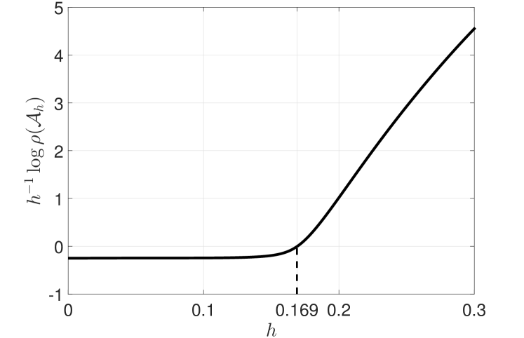
Figure 1: $h^{-1}\log(\rho(\mathcal{A}_{h}))$ versus $h$

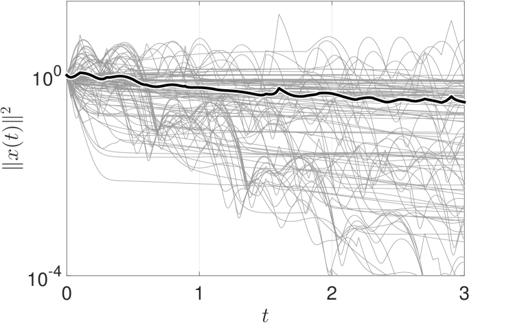
(a) $h=0.1$ (stable)

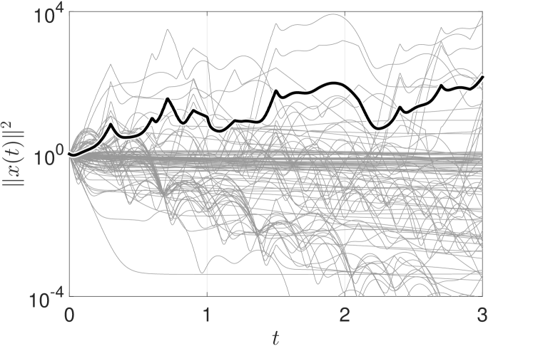
(b) $h=0.3$ (unstable)

Figure 2: Sample paths of $\lVert x(t)\rVert^{2}$ (thin lines) and their averages (thick lines) for $h=0.1$ and $0.3$

In Figs. 2 and 2, we show $100$ sample paths of $\lVert x(t)\rVert^{2}$ and their sample averages when $h=0.1$ and $h=0.3$, respectively. For the generation of each sample path, we take $x_{0}$ randomly from the unit sphere in $\mathbb{R}^{3}$ and $r_{0}$ from the uniform distribution on $\{1,2,3\}$. We can see that mean square stability is achieved with sampling period $h=0.1$, while the closed-loop system exhibits instability for $h=0.3$. Finally, for each value of $h$, we show sample paths of $\sigma=(r,q)$ in Fig. 3. We notice that the change of the values of $q$ occurs only at sampling instants, shown by the dotted lines.

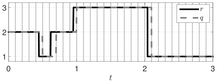
(a) $h=0.1$ (stable)

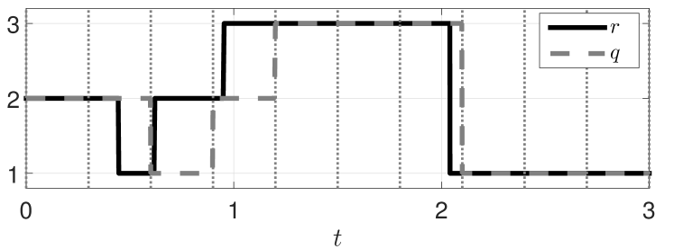
(b) $h=0.3$ (unstable)

Figure 3: Sample paths of $\sigma=(r,q)$ for $h=0.1$ and $0.3$. Solid lines, dashed lines, and dotted lines show $r$, $q$, and sampling instants, respectively.

4 Conclusion

In this paper, we have investigated the mean stability of Markov regenerative switched linear systems. The class of switched linear systems contain a wide variety of important stochastic switched linear systems that have appeared in the literature. We have shown that the mean stability of a Markov regenerative switched linear system is characterized by the spectral radius of a matrix arising from its transition matrix. A numerical example was presented to illustrate the obtained result.

References

- [1] \harvarditem[Antunes et al.]Antunes, Hespanha \harvardand Silvestre2013Antunes2013 Antunes, D. J., Hespanha, J. P. \harvardand Silvestre, C. J. \harvardyearleft2013\harvardyearright, ‘Stochastic hybrid systems with renewal transitions: moment analysis with application to networked control systems with delays’, SIAM Journal on Control and Optimization 51, 1481–1499.
- [2] \harvarditemBlair \harvardand Sworder1975Blair1975 Blair, W. P. \harvardand Sworder, D. D. \harvardyearleft1975\harvardyearright, ‘Continuous-time regulation of a class of econometric models’, IEEE Transactions on Systems, Man, and Cybernetics SMC-5, 341–346.
- [3] \harvarditemBrockett1973Brockett1973 Brockett, R. W. \harvardyearleft1973\harvardyearright, ‘Lie theory and control systems defined on spheres’, SIAM Journal on Applied Mathematics 25, 213–225.
- [4] \harvarditemÇinlar1974Cinlar1974 Çinlar, E. \harvardyearleft1974\harvardyearright, ‘Periodicity in Markov renewal theory’, Advances in Applied Probability 6(1), 61–78.
- [5] \harvarditemÇinlar1975Cinlar1975 Çinlar, E. \harvardyearleft1975\harvardyearright, ‘Exceptional paper–Markov renewal theory: A survey’, Management Science 21(7), 727–752.
- [6] \harvarditemCetinkaya \harvardand Hayakawa2015Cetinkaya2014b Cetinkaya, A. \harvardand Hayakawa, T. \harvardyearleft2015\harvardyearright, ‘Feedback control of switched stochastic systems using randomly available active mode information’, Automatica 52, 55–62.
- [7] \harvarditem[Choi et al.]Choi, Kulkarni \harvardand Trivedi1994Choi1994 Choi, H., Kulkarni, V. G. \harvardand Trivedi, K. S. \harvardyearleft1994\harvardyearright, ‘Markov regenerative stochastic Petri nets’, Performance Evaluation 20, 337–357.
- [8] \harvarditem[Costa et al.]Costa, Fragoso \harvardand Todorov2013Costa2013 Costa, O. L. V., Fragoso, M. D. \harvardand Todorov, M. G. \harvardyearleft2013\harvardyearright, Continuous-time Markov Jump Linear Systems, Springer.
- [9] \harvarditemDistefano \harvardand Trivedi2013Distefano2013 Distefano, S. \harvardand Trivedi, K. S. \harvardyearleft2013\harvardyearright, ‘Non-Markovian state-space models in dependability evaluation’, Quality and Reliability Engineering International 29, 225–239.
- [10] \harvarditemFang \harvardand Loparo2002Fang2002c Fang, Y. \harvardand Loparo, K. \harvardyearleft2002\harvardyearright, ‘Stabilization of continuous-time jump linear systems’, IEEE Transactions on Automatic Control 47(10), 1590–1603.
- [11] \harvarditemFarina \harvardand Rinaldi2000Farina2000 Farina, L. \harvardand Rinaldi, S. \harvardyearleft2000\harvardyearright, Positive Linear Systems: Theory and Applications, Wiley-Interscience.
- [12] \harvarditem[Hou et al.]Hou, Luo \harvardand Shi2005Hou2005 Hou, Z., Luo, J. \harvardand Shi, P. \harvardyearleft2005\harvardyearright, ‘Stochastic stability of linear systems with semi-Markovian jump parameters’, The ANZIAM Journal 46, 331–340.
- [13] \harvarditemOgura \harvardand Martin2014Ogura2013f Ogura, M. \harvardand Martin, C. F. \harvardyearleft2014\harvardyearright, ‘Stability analysis of positive semi-Markovian jump linear systems with state resets’, SIAM Journal on Control and Optimization 52, 1809–1831.
- [14] \harvarditemOgura \harvardand Martin2015Ogura2014d Ogura, M. \harvardand Martin, C. F. \harvardyearleft2015\harvardyearright, ‘Stability analysis of linear systems subject to regenerative switchings’, Systems & Control Letters 75, 94–100.
- [15] \harvarditemParrilo \harvardand Jadbabaie2008Parrilo2008 Parrilo, P. A. \harvardand Jadbabaie, A. \harvardyearleft2008\harvardyearright, ‘Approximation of the joint spectral radius using sum of squares’, Linear Algebra and its Applications 428, 2385–2402.
- [16] \harvarditem[Seidman et al.]Seidman, Schneider \harvardand Arav2005Seidman2005 Seidman, T. I., Schneider, H. \harvardand Arav, M. \harvardyearleft2005\harvardyearright, ‘Comparison theorems using general cones for norms of iteration matrices’, Linear Algebra and its Applications 399, 169–186.
- [17] \harvarditemSigman \harvardand Wolff1993Sigman1993 Sigman, K. \harvardand Wolff, R. W. \harvardyearleft1993\harvardyearright, ‘A Review of regenerative processes’, SIAM Review 35, 269–288.
- [18] \harvarditemSmith1955Smith1955 Smith, W. L. \harvardyearleft1955\harvardyearright, ‘Regenerative stochastic processes’, Proceedings of the Royal Society A: Mathematical, Physical and Engineering Sciences 232(1188), 6–31.
- [19] \harvarditemTam \harvardand Schneider2006Tam2006 Tam, B.-S. \harvardand Schneider, H. \harvardyearleft2006\harvardyearright, Matrices Leaving a Cone Invariant, in L. Hogben, ed., ‘Handbook of Linear Algebra’, Chapman & Hall/CRC, chapter 26.
- [20]