Exact solutions for chemical concentration waves of self-propelling camphor particles racing on a ring: A novel potential dynamics perspective

Abstract

A potential dynamics approach is developed to determine the periodic standing and traveling wave patterns associated with self-propelling camphor objects floating on ring-shaped water channels. Exact solutions of the wave patterns are derived. The bifurcation diagram describing the transition between the immobile and self-propelling modes of camphor objects is derived semi-analytically. The bifurcation is of a pitchfork type which is consistent with earlier theoretical work in which natural boundary conditions have been considered.

Key words: chemical concentration waves, self-motion, pitchfork bifurcation

PACS: 05.45.-a, 82.40.Ck

Abstract

Розвинуто метод потенцiальної динамiки для того, щоб вивчити картини перiодичних стоячих i бiжучих хвиль, пов’язаних iз самоурухомлювальними камфорними об’єктами, якi рухаються на кiльцеподiбних водяних каналах. Отримано точнi розв’язки хвильвових картин. Отримано напiваналiтично дiаграму бiфуркацiї, яка описує перехiд мiж нерухомою i самоурухомлювальною модами камфорних об’єктiв. Бiфуркацiя є вилоподiбна, що узгоджується з попередньою теоретичною роботою, в якiй розглянуто природнi граничнi умови.

Ключовi слова: хвилi хiмiчної концентрацiї, саморух, вилоподiбна бiфуркацiя

1 Introduction

A challenge in modern-day research in biophysics and bioengineering is to create and understand biochemical particle systems that mimic biological cell motion. In particular, at issue is to construct particles-surface systems in which particles have the capability to move themselves over certain distances by converting chemical energy into kinetical energy [1]. As pointed out in reference [1], a fundamental class of such man-made self-moving systems is given by objects that are floating on a medium, are driven by differences in the surface tension of that medium, and at the same time produce gradients of some substance that affects the surface tension of the medium. Irrespective of engineering applications, self-propelling chemical systems allow us to study principles that might be important for our understanding of the physics of life, in general, and the so-called active Brownian particles [2], in particular. In fact, it has been shown that under certain conditions self-propelling chemical ‘‘motors’’ exhibit negative friction terms [1, 3] that are a hallmark of active Brownian systems [2, 4, 5, 6, 7, 8]. A variety of self-propelling chemical motors have been studied [3, 9, 10, 11, 12, 13, 14]. In particular, the self-motion of camphor particles moving on water has been extensively studied, in particular, by Nakata and colleagues [15, 16, 17, 18, 19, 20]. In this context, we would like to point out that not only single camphor particles have been considered but also the interaction between two self-propelling camphor particles has been examined [21], the collective motion of a small number (about 10) of camphor particles has been investigated [22, 23], and the spatial and velocity distributions of many interacting camphor particles have been determined [24, 25].

A theoretical model for the self-motion of a single, solid camphor disc floating on water has been developed in terms of a Newtonian equation for the disc and a reaction-diffusion equation for the concentration of the surface-tension active camphor molecules on the water surface [26]. In this context, analytical solutions of the concentration wave patterns under natural boundary conditions have been derived and it has been shown that the self-propelling mode bifurcates from an immobile mode by means of a pitchfork bifurcation. However, an experimentally very useful paradigm is the self-motion of a camphor disc on a ring channel [15, 16, 17, 18, 19, 20].

In view of the importance of ring-shaped designs for experimental research, the present study goes beyond the case of natural boundary conditions. To the best of our knowledge, we will for the first time present a theoretical analysis of the periodic case that can directly be applied to and compared with the laboratory situation. In addition, while it is plausible to assume that the chemical wave patterns of camphor particles on a ring exhibit a single peak, a clear explanation why this should be the case has not been given so far. Such an explanation will be given below. To this end, a potential dynamic perspective for the coupled particle-wave system will be developed.

Explicitly, the aim of the current study is threefold. First, we will work out a potential dynamics approach to wave patterns of reaction-diffusion systems in order to qualitatively discuss the possible shapes of the camphor concentration patterns associated with the self-motion of camphor discs floating on a ring channel. Second, we will derive analytical solutions for the standing and traveling concentration waves associated with immobile and self-propelling camphor discs, respectively, on a ring channel. Third, we will numerically determine the bifurcation diagram for the case of periodic boundary conditions. In doing so, we will show that the pitchfork bifurcation derived earlier for natural boundary conditions can also be found in the case of periodic boundary conditions that is frequently used in experimental research.

We consider a camphor disc traveling on a ring channel filled with water. Note that the disc releases camphor to the water surface, which implies that in this system we need to distinguish between the camphor disc and the camphor concentration on the water surface. The width of the ring channel is of the disc diameter such that the disc can move only in one direction, along the ring. The ring has radius $R$ and circumference $2\pi R$. The disc position is described by the periodic variable $y(t)\in[0,2\pi R]$, where $t$ denotes time. Moreover, the velocity of the disc is described by $v(t)$. The concentration $u$ of camphor molecules on the water surface at time $t$ and at a particular position $x\in[0,2\pi R]$ along the ring is described by the field variable $u(x,t)\geqslant 0$. The dynamics of the camphor disc is given by [26]

$$\frac{{\mathrm{d}}}{{\mathrm{d}}t}y=v,$$ (1.1a)

$$\frac{{\mathrm{d}}}{{\mathrm{d}}t}v=-\frac{a\gamma}{(au+1)^{2}}\frac{\partial}{\partial x}u\bigg{|}_{x=y(t)}-\mu\,v$$ (1.1b)

with $a,\gamma,\mu>0$. Accordingly, the disc satisfies a Newtonian equation with a force generated by the camphor concentration field $u$ and a friction force proportional to the camphor disc velocity. From a mechanistic point of view, the camphor concentration affects the surface tension, which in turn acts as a force on the camphor disc (see introduction above). The effective force given as the first term on the right hand side of equation (1.1b) can be regarded as a gradient force of a potential, where $u$ is the potential. That is, the camphor disc is driven away from regions of high camphor concentrations. The parameters $\gamma$ and $a$ are related to certain details of the aforementioned mechanistic relationship between camphor concentration, surface tension, and the force acting on the camphor particle, see reference [26]. Finally, in equation (1.1) the parameter $\mu$ denotes the friction coefficient. The camphor concentration field $u(x,t)$ satisfies the reaction-diffusion equation

$$\frac{\partial}{\partial t}u=\frac{\partial^{2}}{\partial x^{2}}u-k\,u+F(x-y(t))$$ (1.2)

with $k>0$. The term $-k\,u$ describes the decay of the camphor concentration on the water surface due to dissolution and sublimation. The function $F$ describes the increase of camphor concentration on the water surface due to the camphor disc depositing camphor molecules to the water surface. Mathematically speaking, $F$ corresponds to a source term. In this context, note that we consider not too long time periods during which the mass loss of the camphor disc can be neglected. The source term $F$ is defined by $F=1$ for $|\Delta|\leqslant r$ and $\Delta=x-y$ and $F=0$ otherwise, where $r>0$ is the radius of the camphor disc. Note that from a mathematical point of view for large $r$ we may not think of the disc as a circular object. We may imagine a solid object that has the shape of a segment of the ring with segment length $2r$ measured along the curvilinear coordinate $x$. Then, we have $r\leqslant\pi R$. In the case $r=\pi R$, the object would be a full, solid ring that covers the whole surface of the ring channel.

It is important to note that equations (1.1) and (1.2) actually represent rescaled equations such that the variables $x$, $y$, $u$, and even the time variable $t$ are given in dimensionless units. For example, the (real world) laboratory time $t_{\textrm{lab}}$ measured in seconds is given by the dimensionless time $t$ occurring in equations (1.1) and (1.2) divided by a rate constant measured in 1/sec that describes the rate with which camphor is released from the camphor disc to the water surface [26].

2 Potential dynamics perspective of the chemical wave pattern associated with a self-propelling camphor disc

2.1 Potential dynamics point of view

The objective is to study traveling wave solutions [27, Sec. 7.3] of the form

$$u(x,t)=g(x-c\,t)$$ (2.1)

of the model defined by equations (1.1) and (1.2), where $c$ is the velocity of the traveling wave. Let us define $z=x-c\,t$ as the phase coordinate of the wave. The reaction diffusion equation (1.1) describes a standing or traveling wave pattern only if the source $F$ depends on the phase coordinate $z$ rather than on $x$ and $y(t)$. Substituting $z=x-ct$ into $\Delta=x-y(t)$, we obtain $\Delta=z+c\,t-y(t)$. The requirement that $\Delta$ depends only on $z$ implies that $y(t)=c\,t+y_{0}$ with $y_{0}\in[2\pi R]$. This also leads to $v(t)=c$. The camphor disc moves with the same velocity as the wave pattern. Substituting equation (2.1) into equation (1.2), we obtain

$$\frac{\partial^{2}}{\partial z^{2}}g=-c\frac{\partial}{\partial z}g-k\,g+F(z-y_{0})\,.$$ (2.2)

Likewise, from equation (1.1) it follows that

$$\frac{\partial}{\partial z}g\bigg{|}_{z=y_{0}}=-\frac{\mu\,c}{a\gamma}[ag(y_{0})+1]^{2}\,.$$ (2.3)

The position $y_{0}$ of the camphor disc is arbitrary. That is, if there is a wave pattern $g(z,y_{0})$ with a particular camphor disc position $y_{0}$, then $y_{0}+h$ has the solution $g(z,y_{0}+h)=g(z-h,y_{0})$, which shifts the wave pattern by $h$. Without loss of generality, we put $y_{0}=0$ such that

$$\frac{{\mathrm{d}}^{2}}{{\mathrm{d}}z^{2}}g=-c\frac{\partial}{\partial z}g-k\,g+F(z)$$ (2.4)

and

$$\frac{{\mathrm{d}}}{{\mathrm{d}}z}g\bigg{|}_{z=0}=-\frac{\mu\,c}{a\gamma}[ag(0)+1]^{2}$$ (2.5)

with $F=1$ if $z\in[0,r]\cup[2\pi R\!-\!r,2\pi R]$ and $F=0$ otherwise. The wave pattern is subjected to periodic boundary conditions $g(z)=g(z+2\pi R)$, which implies that the relations $g(0)=g(2\pi R)$ and ${\mathrm{d}}g(0)/{\mathrm{d}}z={\mathrm{d}}g(2\pi R)/{\mathrm{d}}z$ hold. The traveling wave equations (2.4) and (2.5) contain the standing wave equations as special case. For the standing wave we put $c=0$ such that

$$\frac{{\mathrm{d}}^{2}}{{\mathrm{d}}z^{2}}g=-k\,g+F(z)$$ (2.6)

and

$$\frac{{\mathrm{d}}}{{\mathrm{d}}z}g\bigg{|}_{z=0}=0\,.$$ (2.7)

These equations have a symmetric solution $g(z)=g(-z)$.

Equations (2.4)–(2.7) can be solved using the potential dynamics method for solving reaction-diffusion equations (see e.g. reference [28, Chap. 9]). Accordingly, $g$ is regarded as the position of a hypothetical point particle that evolves in time $t$ and moves with a particle velocity $v_{g}$. In doing so, the phase coordinate $z$ is replaced by the time variable $t$. The particle motion is subjected to a potential force with a potential $V(g,t)$ that depends on time. Using these replacements [i.e., $z\to t$ and ${\mathrm{d}}g/{\mathrm{d}}z\to v_{g}(t)$], equation (2.4) becomes

$$\frac{{\mathrm{d}}}{{\mathrm{d}}t}g=v_{g}\,,\qquad\frac{{\mathrm{d}}}{{\mathrm{d}}t}v_{g}=-c\,v_{g}-\frac{\partial}{\partial g}V(g,t)$$ (2.8)

and we are looking for periodic solutions $g(t)$ with period $T=2\pi R$. During the time intervals $[0,r]$ and $[T-r,T]$ we have $F=1$ and the potential $V$ gives rise to the ‘‘force’’ $-{\mathrm{d}}V/{\mathrm{d}}g=kg-1$. By contrast, for $t\in(r,T-r)$ we have $F=0$ which implies $-{\mathrm{d}}V/{\mathrm{d}}g=kg$. In total, the potential is given by

$$V(g,t)=\left\{\begin{array}[]{lll}-0.5k(g-1/k)^{2}&\text{for}&t\in\{[0,r]\cup[T-r,T]\}_{\text{modulus}\ T}\,,\\ -0.5kg^{2}&\text{for}&t\ \text{otherwise}\,.\end{array}\right.$$ (2.9)

The two different potential forms described by equation (2.9) are illustrated in figure 1 and will be referred to as type I and II potentials, respectively. Both potentials are inverted parabolic potentials. For $t\in\{[0,r]\cup[T-r,T]\}$ the potential has a peak at $g=1/k$ (top panel), otherwise the potential has a peak at $g=0$ (bottom panel). Equations (2.8) and (2.9) have to be solved under initial conditions $g(t=0)$ and $v_{g}(t=0)$ that satisfy

$$v_{g}(t=0)=-\frac{\mu\,c}{a\gamma}[a\,g(t=0)+1]^{2}\ ,$$ (2.10)

see equation (2.5). Moreover, the periodicity condition $g(t+T)=g(t)$ implies that the boundary conditions $g(t=0)=g(t=T)$ and $v_{g}(t=0)=v_{g}(t=T)$ hold. Finally, we have the constraint $g(t)\geqslant 0$ because $g$ in the original context reflects the concentration of camphor molecules. The potential dynamics subjected to these initial and boundary conditions is then determined by the two types of repulsive potentials shown in figure 1.

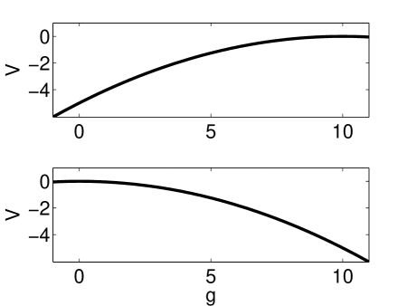
Figure 1: Potentials of type I (top) and II (bottom) defined by equation (2.9). Here $k=0.1$.

Let us discuss period solutions $g(t)$ corresponding to standing wave patterns $g(z)$ associated with an immobile camphor disc. For $c=0$, equation (2.9) describes a Newtonian equation without damping that is solved under the initial conditions $v_{g}=0$ and $g(0)=A>0$. If $A>1/k$, then we have $g\to\infty$ for $t\to\infty$ because both potentials decay monotonously for $g>1/k$. For $g(0)=1/k$, a periodic solution is not possible for $0<r<\pi R$. However, in the limiting case $r=\pi R$, the dynamics of the hypothetical particle is subjected only to the potential I force with $V_{\textrm{max}}=1/k$ (top panel of figure 1) such that $g(0)=g(t)=1/k$ is the solution of equation (2.9). That is, the wave pattern $g(z)$ is a constant when the water channel is completely filled with a solid, ring-shaped camphor object. In summary, for $0<r<\pi R$ we have $g(0)=A\in(0,1/k)$. Due to the potential I force, for $t\in[0,r]$, the particle moves ‘‘downhill’’ with respect to the type I potential $V$, that is, to the left towards $g=0$, and reaches at time $t=r$ a point $g(r)=B$. At $t=r$, the potential switches from type I to type II. Since we have $v_{g}(r)<0$, the particle continues to move towards $g=0$. However, at this stage it moves ‘‘uphill’’ with respect to the type II potential $V$ and, consequently, is de-accelerated. At a time point $t^{*}$, the particle has zero velocity ($v_{g}(t^{*})=0$). At this instance, the particle has reached its minimal position $g(t^{*})=g_{\textrm{min}}$. Due to the impact of the potential II force, the particle is accelerated and starts to move ‘‘downhill’’ with respect to the type II potential $V$, that is, it moves to the right. Due to the symmetry of the problem at hand, the time point $t^{*}$ is half of the period: $t^{*}=T/2=\pi R$. When the particle moves to the right, $g$ increases and eventually, at $t=T-r$, the particle reaches the position $g=B$ again. Note that the ‘‘uphill’’ movement $B\to g_{\textrm{min}}$ and the ‘‘downhill’’ movement $g_{\textrm{min}}\to B$ are described by a time-reversible Newtonian equation, which implies that the trajectory $g(t)$ is symmetric with respect to $t=T/2$. At $t=T-r$ we have $v_{g}>0$. In particular, we have $v_{g}(T-r)=-v_{g}(r)$. Moreover, the potential switches from type II to type I. Due to the ‘‘initial’’ velocity $v_{g}(T-r)>0$, the particle goes ‘‘uphill’’ in the type I potential $V$, slows down, and finally reaches the location $g=A$ with $v_{g}=0$ at time point $t=T$. In short, the periodic solution follows the sequence

$$g(0)\!=\!g_{\textrm{max}}\to g(r)\!=\!B\to g(T/2)\!=\!g_{\textrm{min}}\to g(T\!-\!r)\!=\!B\to g(T)\!=\!g(0)$$

and exhibits a single maximum at $g(0)$ and a single minimum at $g(T/2)$. Moreover, the trajectory is symmetric with respect to $t=T/2$ for $t\in[0,T]$ (and symmetric with respect to $t=0$ for $t\in[-T/2,T/2]$), which means that the periodic standing wave pattern $g(z)$ has a symmetry axis.

Periodic solutions with $v_{g}(0)\neq 0$ related to traveling wave patterns $g(z)$ induced by a self-propagating camphor disc can be discussed in a similar way. In this context, we note that a necessary condition for a period solution is $g(0)<1/k$ again. In order to see this, let us assume that $g(0)>1/k$ holds. For $c<0$, this implies $v_{g}(0)>0$ which implies $g\to\infty$ for $t\to\infty$ because both potentials I and II decay monotonously for $g>1/k$. For $c>0$ and $g(0)>1/k$, we see that the particle has initial velocity $v_{g}(0)<0$ and moves towards $g=1/k$, which is the peak of the type I potential $V$ (figure 1, top panel). If $|v_{g}(0)|$ is not sufficiently large, it will not reach the point $g=1/k$. Rather, we will have $v_{g}(t^{\prime})=0$ with $g(t^{\prime})>1/k$ for $t^{\prime}\in[0,r]$ which implies $g\to\infty$ to $t\to\infty$. That is, a necessary condition for a periodic solution starting at $g(0)>1/k$ is that $|v_{g}(0)|$ is sufficiently large such that the particle passes the point $g=1/k$ during the interval $[0,r]$. However, the particle should return somehow to the initial position $g(0)>1/k$. Once the particle has passed the point $g=1/k$ at $t^{\prime}\in[0,r]$, the only way to return to the subspace $g=(1/k,\infty)$ is to pass the point $g=1/k$ at a later time point $t^{\prime\prime}>t^{\prime}$ with velocity $v_{g}(t^{\prime\prime})>0$. From $g(t^{\prime\prime})=1/k$ and $v_{g}(t^{\prime\prime})>0$ it follows that $g\to\infty$ for $t\to\infty$. In summary, periodic solutions with $v_{g}(0)\neq 0$ and $g>0$ only exist for $g(0)\in(0,1/k)$. By analogy to the previous discussion for the case $c=v_{g}(0)=0$, for $c>0$ (camphor disc and wave pattern traveling to the right on the ring coordinate $x$) we obtain the sequence

$$g(0) =A\to g(r)=B<A\,\to\,g(t^{*})=g_{\textrm{min}}<B\,\to\,g(T-r)=C>g_{\textrm{min}}$$

$$\to g(t^{**})=D=g_{\textrm{max}}>A\to g(T)=g(0)=A$$ (2.12)

with $0<r<t^{*}<T-r<t^{**}<T$ and $v_{g}=0$ at $t^{*}$ and $t^{**}$. As indicated, the maximum is reached at $t^{**}\in[T-r,T]$ and does not correspond to the initial position $g(0)$. In any case, there is a single minimum and a single maximum, which means that a traveling wave concentration pattern $g(z)$ is single-peaked and exhibits a single minimum. The condition $g(t^{**})>g(T)=g(0)$ implies for the original problem that the camphor disc is located to the ‘‘right’’ of the peak of the traveling wave concentration pattern. For $c<0$, we conclude in a similar vein that the traveling wave pattern is single-peaked and has a single minimum. As anticipated above, the potential dynamic picture reveals that both the standing and traveling wave patterns exhibit a single peak only. However, while the standing wave patterns $g(z)$ exhibit a symmetry axis, traveling wave patterns $g(z)$ are non-symmetric.

The next objective is to explicitly formulate the scenarios described by the sequences (2.1) and (2.1) in order to obtain analytical solutions for $g(t)$ and for the patterns $g(z)$.

2.2 Standing waves

We will derive the next symmetric solutions of equation (2.8) with $v_{g}(0)=0$. In this case, it is sufficient to determine the trajectory $g(t)$ in the interval $[0,T/2=\pi R]$ because, as we will see below we can take advantage of the constraint $v_{g}(T/2)=0$, see equation (2.1). For $t\in[0,r]$, the solution $g(t)$ satisfies equation (2.8) with $c=0$, $v_{g}(0)=0$, and $g(0)\in(0,1/k)$. The solution reads

$$g(t)=\left[g(0)-\frac{1}{k}\right]\cosh(\sqrt{k}t)+\frac{1}{k}\,.$$ (2.13)

In particular, we obtain

$$g(r)=\left[g(0)\!-\!\frac{1}{k}\right]\cosh(\sqrt{k}r)\!+\!\frac{1}{k}\,,\qquad v_{g}(r)=\sqrt{k}\left[g(0)\!-\!\frac{1}{k}\right]\sinh(\sqrt{k}r)\,.$$ (2.14)

For $t\in(r,T/2]$ the solution $g(t)$ satisfies equation (2.8) for $c=0$ and the initial conditions $g(r)$ and $v_{g}(r)$ given above. The solution reads

$$g(t) = \frac{1}{2}\left[g(r)+\frac{v_{g}(r)}{\sqrt{k}}\right]\exp\left[\sqrt{k}(t\!-\!r)\right]+\frac{1}{2}\left[g(r)-\frac{v_{g}(r)}{\sqrt{k}}\right]\exp\left[-\sqrt{k}(t\!-\!r)\right]$$ (2.15)

$$= g(r)\cosh\left[\sqrt{k}(t-r)\right]+\frac{v_{g}(r)}{\sqrt{k}}\sinh\left[\sqrt{k}(t-r)\right]\,,$$

which implies that

$$v_{g}(t)=\sqrt{k}g(r)\cosh\left[\sqrt{k}(t-r)\right]+v_{g}(r)\cosh\left[\sqrt{k}(t-r)\right]\,.$$ (2.16)

The functions (2.13)–(2.16) involve the unknown parameter $g(0)$. Let us use the constraint $v_{g}(T/2)=0$ to determine $g(0)$. Substituting $t=\pi R$ with $v_{g}(t=\pi R)=0$ into equation (2.16) and substituting equation (2.14) into equation (2.16) as well, we obtain

$$\xi\,w=-\frac{1}{k}\sinh\left[\sqrt{k}(\pi R-r)\right]<0$$ (2.17)

with $\xi=g(0)-1/k$ and

$$w=\sinh(\sqrt{k}r)\cosh\left[\sqrt{k}(\pi R-r)\right]+\cosh(\sqrt{k}r)\sinh\left[\sqrt{k}(\pi R-r)\right]>0\,.$$

Since the right hand side of equation (2.17) is negative and $w>0$, we conclude that $\xi<0$. In addition, we see that

$$g(0)=\xi+\frac{1}{k}=\frac{1}{k}\left\{1-\frac{\sinh\left[\sqrt{k}(\pi R-r)\right]}{w}\right\}$$ (2.19)

holds. From $w>\sinh[\sqrt{k}(\pi R-r)]$ it follows that the factor $\sinh[\sqrt{k}(\pi R-r)]/w>0$ is smaller than 1 such that $g(0)\in(0,1/k)$. That is, $g(0)$ satisfies the necessary condition for periodic solutions.

Equations (2.13)–(2.15) in combination with the initial condition (2.19) describe the analytical solution $g(t)$ in $t\in[0,T/2]$. As shown above, solutions of equation (2.8) with $c=0$ and $v_{g}(0)=0$ are symmetric with respect to $t=0$ (and $t=T/2$). Consequently, solutions on a full period are given by $g(t)$ defined by equations (2.13)–(2.15) and (2.19) for $t\in[0,T/2]$ and $g(t)=g(-t)$ for $t\in[-T/2,0]$. Likewise the pattern of the standing wave solution $g(z)$ can be computed from equations (2.13)–(2.15) and (2.19) for $z\in[0,\pi R]$ and $g(z)=g(-z)$ for $z\in[-\pi R,0]$.

Figure 2 shows $g(z)$ for a standing wave pattern. The solid line was obtained from equations (2.13)–(2.15) and (2.19) and $g(z)=g(-z)$. The circles were obtained by solving equation (2.8) numerically in the interval $t\in[0,T/2]$ with initial condition $v_{g}(0)=0$ by means of an Euler forward algorithm for the dynamics of a Newtonian particle (single time step $10^{-5}$). Numerical and analytical solution methods showed consistent results. Although the peak of the pattern shown in figure 2 looks kinky, from equations (2.13)–(2.15) it follows that in fact the functions $g(t)$ and $g(z)$ are smooth functions at $t=z=0$ (i.e., continuously differentiable). This is illustrated in the insert of figure 2 that depicts the standing wave pattern in a small region around $z=0$.

Let us briefly address the case $r\to\pi R$. For $r=\pi R$ equation (2.13) yields $g(t)=1/k$. Likewise, equation (2.19) reduces to $g(0)=1/k$. This is consistent with the conclusion drawn above that for $r=\pi R$ the ring channel exhibits a homogeneous concentration pattern $g=1/k$.

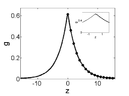
Figure 2: Standing wave solution $g$ (solid line) computed from the analytical solution defined by equations (2.13)–(2.15) and (2.19). Circles correspond to the graph $g$ determined by a numerical solution method (see text). Insert shows a detail of the graph $g(z)$ around $z=0$. Parameters: $k=0.1$, $R=5.0$, $r=0.2$ (as in reference [26]).

2.3 Traveling waves

Our next objective is to find solutions of equations (2.8)–(2.10) for $c\neq 0$ which implies $v_{g}(0)\neq 0$. To this end, we will use equations (2.8) and (2.9) to determine the trajectory $g(t)$ and the particle velocity $v_{g}(t)$ in the full period $[0,T]$ as function of the unknown parameters $g(0)$, $v_{g}(0)$ and $c$. We will then use the three constraints given by equation (2.10) and by the two periodicity requirements $g(0)=g(T)$ and $v_{g}(0)=v_{g}(T)$ to determine $g(0)$, $v_{g}(0)$ and $c$.

For $t\in[0,r]$, equation (2.8) explicitly reads $\mathrm{d}^{2}g/{\mathrm{d}}t^{2}=-cv_{g}+kg-1$. The solution involves the unknown parameters $c$, $v_{g}(0)$, and $g(0)$ and reads

$$g(t)=A_{1,0}\exp\{\lambda_{1}t\}+A_{2,0}\exp\{\lambda_{2}t\}+\frac{1}{k}$$ (2.20)

with eigenvalues

$$\lambda_{1}(c)=-\frac{c}{2}+\sqrt{\frac{c^{2}}{4}+k}>0\,,\qquad\lambda_{2}(c)=-\frac{c}{2}-\sqrt{\frac{c^{2}}{4}+k}<0$$ (2.21)

and amplitudes

$$A_{1,0}=\left[g(0)-\frac{1}{k}-\frac{v_{g}(0)}{\lambda_{2}}\right]\frac{1}{1-\lambda_{1}/\lambda_{2}}\,,$$

$$A_{2,0}=\left[g(0)-\frac{1}{k}-\frac{v_{g}(0)}{\lambda_{1}}\right]\frac{1}{1-\lambda_{2}/\lambda_{1}}\,.$$ (2.22)

In particular, we obtain

$$g(r) = A_{1,0}\exp\{\lambda_{1}r\}+A_{2,0}\exp\{\lambda_{2}r\}+\frac{1}{k}\,,$$

$$v_{g}(r) = A_{1,0}\lambda_{1}\exp\{\lambda_{1}r\}+A_{2,0}\lambda_{2}\exp\{\lambda_{2}r\}\,.$$ (2.23)

For $t\in(r,T-r)$, equation (2.8) explicitly reads ${\mathrm{d}}^{2}g/{\mathrm{d}}t^{2}=-cv_{g}+kg$. The solution involves the initial conditions $g(r)$ and $v_{g}(r)$ listed above and reads

$$g(t)=A_{1,r}\exp\{\lambda_{1}(t-r)\}+A_{2,r}\exp\{\lambda_{2}(t-r)\}$$ (2.24)

with the amplitudes

$$A_{1,r}=\left[g(r)-\frac{v_{g}(r)}{\lambda_{2}}\right]\frac{1}{1-\lambda_{1}/\lambda_{2}}\,,\qquad A_{2,r}=\left[g(r)-\frac{v_{g}(r)}{\lambda_{1}}\right]\frac{1}{1-\lambda_{2}/\lambda_{1}}\,.$$

In particular, we obtain

$$g(T-r) = A_{1,r}\exp\{\lambda_{1}(T-2r)\}+A_{2,r}\exp\{\lambda_{2}(T-2r)\}\,,$$

$$v_{g}(T-r) = A_{1,r}\lambda_{1}\exp\{\lambda_{1}(T-2r)\}+A_{2,r}\lambda_{2}\exp\{\lambda_{2}(T-2r)\}\,.$$ (2.26)

Finally, for $t\in[T-r,T]$ equation (2.8) explicitly reads ${\mathrm{d}}^{2}g/{\mathrm{d}}t^{2}=-cv_{g}+kg-1$. The solution involves the initial conditions $g(T-r)$ and $v_{g}(T-r)$ (determined above) and reads

$$g(t)=A_{1,T-r}\exp\{\lambda_{1}[t-(T-r)]\}+A_{2,T-r}\exp\{\lambda_{2}[t-(T-r)]\}+\frac{1}{k}$$

with amplitudes

$$A_{1,T-r}=\left[g(T-r)-\frac{1}{k}-\frac{v_{g}(T-r)}{\lambda_{2}}\right]\frac{1}{1-\lambda_{1}/\lambda_{2}}\,,$$

$$A_{2,T-r}=\left[g(T-r)-\frac{1}{k}-\frac{v_{g}(T-r)}{\lambda_{1}}\right]\frac{1}{1-\lambda_{2}/\lambda_{1}}\,.$$ (2.28)

In particular, we obtain

$$g(T) = \underbrace{A_{1,T-r}\exp\{\lambda_{1}r\}+A_{2,T-r}\exp\{\lambda_{2}r\}+\frac{1}{k}}_{\displaystyle f_{1}}\,,$$

$$v_{g}(T) = \underbrace{A_{1,T-r}\lambda_{1}\exp\{\lambda_{1}r\}+A_{2,T-r}\lambda_{2}\exp\{\lambda_{2}r\}}_{\displaystyle f_{2}}\,.$$ (2.29)

As mentioned above, we put $g(0)=g(T)$ and $v_{g}(0)=v_{g}(T)$ such that

$$g(0)=f_{1}\big{(}g(0),v_{g}(0),c\big{)}\ ,\ v_{g}(0)=f_{2}\big{(}g(0),v_{g}(0),c\big{)}\ .$$ (2.30)

The functions $f_{1}$ and $f_{2}$ occurring in equation (2.30) are defined by the expressions on the right hand sides of equation (2.3) and by the amplitudes and initial conditions listed in table 1. These amplitudes and initial conditions are explicitly defined by equations (2.3), (2.3), (2.3), (2.3) and (2.3) with the eigenvalues $\lambda_{1}$ and $\lambda_{2}$ given by equation (2.21).

Table 1: Amplitude and ‘‘initial conditions’’ involved in the definition of the functions $f_{1}$ and $f_{2}$ occurring in equations (2.3) and (2.30).

Amplitudes		Initial conditions
$A_{1,T-r}[g(t-r),v_{g}(T-r),c]$		$g(T-r)[A_{1,r},A_{2,r},c]$
$A_{2,T-r}[g(t-r),v_{g}(T-r),c]$		$v_{g}(T-r)[A_{1,r},A_{2,r},c]$
$A_{1,r}[g(r),v_{g}(r),c]$		$g(r)[A_{1,0},A_{2,0},c]$
$A_{2,r}[g(r),v_{g}(r),c]$		$v_{g}(r)[A_{1,0},A_{2,0},c]$
$A_{1,0}[g(0),v_{g}(0),c]$
$A_{2,0}[g(0),v_{g}(0),c]$

The two relations in equation (2.30) together with the constraint (2.10) provide three equations to determine the parameters $g(0)$, $v_{g}(0)$, and $c$. Once $g(0)$, $v_{g}(0)$, and $c$ have been determined, the trajectory $g(t)$ can be computed from equations (2.20), (2.24) and (2.3). In doing so, the analytical solution for the traveling wave pattern $g(z)$ can be found. It can be useful to eliminate $c$ with the help of equation (2.10) like $c=-a\,\gamma\,v_{g}(0)/\{\mu[ag(0)+1]^{2}\}$. Equation (2.30) then becomes

$$g(0)=h_{1}\big{(}g(0),v_{g}(0)\big{)}\ ,\ v_{g}(0)=h_{2}\big{(}g(0),v_{g}(0)\big{)}$$ (2.31)

with

$$h_{1}=f_{1}\big{(}\cdot,c=-a\,\gamma\,v_{g}(0)/\left\{\mu[ag(0)+1]^{2}\right\}\big{)}\,,$$ (2.32)

$$h_{2}=f_{2}\big{(}\cdot,c=-a\,\gamma\,v_{g}(0)/\left\{\mu[ag(0)+1]^{2}\right\}\big{)}\,.$$ (2.33)

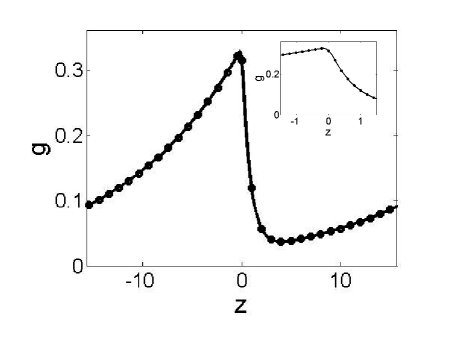
Figure 3: Traveling wave solution $g$ (solid line) computed from the analytical solution defined by equations (2.20), (2.24) and (2.3). Circles were obtained by the same numerical solution method as used in figure 2. Parameters: $a=0.5$, $\gamma=2.0$, $k=0.1$, $R=5.0$, $r=0.2$, $\mu=0.1$ (as in reference [26]). Estimated parameters obtained both from MATLAB fsolve and the $w_{1}(t)$ and $w_{2}(t)$ dynamical system method: $g(0)=0.3151$, $v_{g}(0)=0.1516$, $c=1.1315$.

We numerically solved equation (2.31) for a given set of parameters $a$, $\gamma$, $k$, $R$, $r$, $\mu$ in order to obtain $g(0)$ and $v_{g}(0)$. Subsequently, we calculated $c$ from $c=-a\,\gamma\,v_{g}(0)/\{\mu[ag(0)+1]^{2}\}$. We solved equation (2.31) in two different ways. First, we used the MATLAB solver (fsolve) for coupled nonlinear functions. Second, we numerically solved a dynamical system that exhibits a fixed point consistent with equation (2.31). More precisely, the two-variable dynamical system defined by ${\mathrm{d}}w_{1}(t)/{\mathrm{d}}t=w_{1}-h_{1}(w_{1},w_{2})$ and ${\mathrm{d}}w_{2}(t)/{\mathrm{d}}t=h_{2}(w_{1},w_{2})-w_{2}$ was numerically solved (Euler forward with single time step $10^{-5}$) for initial conditions $w_{1}(0)=0.5/k$ and $w_{2}(0)=-0.1$ (to obtain solutions with $c>0$). For both methods, the same numerical values for $g(0)$, $v_{g}(0)$, and $c$ were obtained up to 4 digits after the decimal point. Subsequently, the traveling wave pattern $g(z)$ was computed from equations (2.20), (2.24) and (2.3). The result is shown in figure 3. A detail of the pattern for values of $z$ close to zero is shown in the insert. We see that the camphor disc at $z=0$ is located to the ‘‘right’’ of the peak of the concentration wave (i.e., the peak position is to the ‘‘left’’ of $z=0$).

Finally, we compute the bifurcation diagram for the same set of parameters $a$, $\gamma$, $k$, $R$, $r$ as used to calculate the wave pattern $g(z)$ in figure 3. However, $\mu$ was not fixed. Rather, the parameter $\mu$ was considered as control parameter and was varied in the range $\mu=[0,0.2]$. The traveling wave velocity $c$ as function of $\mu$ was determined using the two aforementioned methods (MATLAB fsolve and dynamical system $w_{1}(t)$, $w_{2}(t)$). The propagation velocities $c$ thus obtained are shown in figure 4. The bifurcation diagram indicates that for periodic solutions $g(z)$ there is a pitchfork bifurcation at a critical value $\mu_{\textrm{c}}$ such that at $\mu=\mu_{\textrm{c}}$, the standing wave solution with $c=0$ becomes unstable and two stable traveling wave solutions emerge with either $c>0$ or $c<0$.

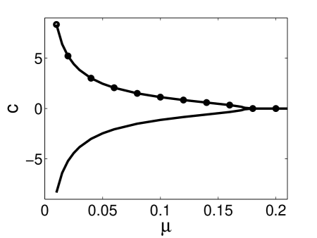
Figure 4: Pitchfork bifurcation describing the transition of a camphor disc floating on a water ring from an immobile mode to a self-motion mode. Two methods were used: MATLAB fsolve (solid line) and dynamical system $w_{1}(t)$, $w_{2}(t)$ (circles). See text for details.

3 Discussion

A potential dynamics approach was used to determine the shape of chemical concentration patterns on a ring-shaped water channel associated with a camphor disc floating on the water surface of the channel either in an immobile or self-propelling fashion. The potential dynamics approach allowed us to qualitatively determine the shape of the wave patterns and to show that the concentration patterns are bounded from above. In rescaled dimensionless units, the maximal camphor concentration of standing or traveling wave patterns cannot exceed the inverse of the decay constant $k$. With the help of the potential dynamics approach, analytical expressions for standing and traveling wave patterns were derived. Finally, by means of the analytical expression for traveling wave patterns, the bifurcation diagram describing the transition from standing to traveling waves (immobility to self-motion) when the friction parameter $\mu$ is decreased was determined numerically.

The stable branches of the bifurcation diagram for values of $\mu$ smaller than the critical value $\mu_{\textrm{c}}$ but close to $\mu_{\textrm{c}}$ (i.e., $\mu=\mu_{\textrm{c}}-\epsilon$ with $\epsilon>0$ small) may be described like $\mu_{\textrm{c}}-\mu=L\,c^{2}+O(c^{4})$, where $L>0$ holds and $c$ corresponds both to the camphor disc velocity and the traveling wave velocity. Taking the immobile-disc and standing-wave solution $c=0$ into account, this relationship between $\mu$ and $c$ becomes $(\mu_{\textrm{c}}-\mu)\,c=L\,c^{3}+O(c^{5})$ and describes a supercritical pitchfork bifurcation. This relationship was analytically derived in a previous study assuming natural boundary conditions [26]. Consequently, our considerations indicate that a supercritical pitchfork bifurcation can also be observed in the case of periodic boundary conditions.

In the aforementioned study it was also shown that under natural boundary conditions and when the radius of the camphor disc becomes large, the velocity $c$ and the control parameter $\mu$ can be related like $(\mu_{\textrm{c}}-\mu)\,c=L_{1}c^{3}+L_{2}c^{5}+O(c^{7})$ with $L_{1}<0$ and $L_{2}>0$. When the solution $c=0$ is ignored, the simplified, truncated relation $\mu_{\textrm{c}}-\mu=L_{1}c^{2}+L_{2}c^{4}$ describes the branches of self-propelling camphor discs associated with traveling wave concentration patterns. It has the shape of a W when considering $\epsilon=\mu_{\textrm{c}}-\mu$ as a function of $c$. Consequently, this second relationship describes a subcritical pitchfork bifurcation when considering $c$ as a function of $\epsilon=\mu_{\textrm{c}}-\mu$. The subcritical bifurcation predicts that for appropriately chosen values of $\mu$, there are two different propagation velocities $c>0$ (and likewise two velocities $c<0$). We were not able to find a counterpart of this observation for the case of periodic boundary conditions. That is, the two numerical methods described in section 2.3 to determine the bifurcation diagram did not indicate the existence of a W shaped relationship between $\mu_{\textrm{c}}-\mu$ and $c$. In this context, it is important to note that in reference [26] it was shown that the range of values $\mu$ for which two different positive (or negative) velocities $c$ exist is relatively small. Therefore, the issue of a subcritical pitchfork bifurcation for solutions of the reaction-diffusion equation (1.2) subjected to periodic boundary conditions may be addressed by more sophisticated analytical or numerical methods that go beyond the scope of the present study.

Ukrainian 0

Точнi розв’язки для хвиль хiмiчної концентрацiї самоурухомлювальних камфорних частинок, що рухаються по кiльцю: нова перспектива потенцiальної динамiки Т.Д. Франк

             
Вiддiл психологiї, Унiверситет м. Коннектикут, CT 06269, США

References

- [1] Mikhailov A.S., Meinköhn D., In: Stochastic Dynamics, Lecture Notes in Physics, Vol. 484, Schimansky-Geier L., Pöschel T. (Eds.), Springer, Berlin, 1997, 334–345.
- [2] Schweitzer F., Brownian agents and active particles, Springer, Berlin, 2003.
- [3] Sumino Y., Yoshikawa K., Chaos, 2008, 18, 026106; doi:10.1063/1.2943646.
-
[4]
Romanczuk P., Bär, Ebeling W., Lindner B., Schimansky-Geier L., Eur. Phys. J.-Spec. Top., 2012, 202, 1;
doi:10.1140/epjst/e2012-01529-y. - [5] Frank T.D., Phys. Lett. A, 2010, 374, 3136; doi:10.1016/j.physleta.2010.05.073.
- [6] Frank T.D., Eur. Phys. J. B, 2010, 74, 195; doi:10.1140/epjb/e2010-00083-8.
- [7] Dotov D.G., Frank T.D., Motor Control, 2011, 15, 550.
- [8] Mongkolsakulvong S., Chaikhan P., Frank T.D., Eur. Phys. J. B, 2012, 85, 90; doi:10.1140/epjb/e2012-20720-4.
- [9] Magome N., Yoshikawa K., J. Phys. Chem., 1996, 100, 19102; doi:10.1021/jp9616876.
- [10] Mano N., Heller A., J. Am. Chem. Soc., 2005, 127, 11574; doi:10.1021/ja053937e.
- [11] Vicario J., Eelkema R., Browne W.R., Meetsma A., La Crois R.M., Feringa B.L., Chem. Commun., 2005, 3936; doi:10.1039/b505092h.
- [12] Kitahata H., Yoshikawa K., Physica D, 2005, 205, 283; doi:10.1016/j.physd.2004.12.012.
- [13] Bassik N., Abebe B.T., Gracias D.H., Langmuir, 2008, 24, 12158; doi:10.1021/la801329g.
- [14] Suematsu N.J., Miyahara Y., Matsuda Y., Nakata S., J. Phys. Chem. C, 2010, 114, 13340; doi:10.1021/jp104666b.
- [15] Nakata S., Hayashima Y., J. Chem. Soc., Faraday Trans., 1998, 94, 3655; doi:10.1039/a806281a.
- [16] Hayashima M., Nagayama M., Nakata S., J. Phys. Chem., 2001, 105, 5353; doi:10.1021/jp004505n.
- [17] Hayashima M., Nagayama M., Doi Y., Nakata S., Kimura M., Iida M., Phys. Chem. Chem. Phys., 2002, 4, 1386; doi:10.1039/b108686c.
- [18] Nakata S., Matsuo K., J. Chem. Soc., Faraday Trans., 2005, 94, 3655; doi:10.1039/a806281a.
- [19] Nakata S., Kirisaka J., Arima Y., Ishii T., J. Phys. Chem. B, 2006, 110, 21131; doi:10.1021/jp063827+.
- [20] Suematsu N.J., Ikura Y., Nagayama M., Kitahuta H., Kawagishi N., Marukami M., Nakata S., J. Phys. Chem. C, 2010, 114, 9876; doi:10.1021/jp101838h.
- [21] Kohira M.I., Hayashima Y., Nagayama M., Nakata S., Langmuir, 2001, 17, 7124; doi:10.1021/la010388r.
- [22] Suematsu N.J., Nakata S., Awazu A., Nishimori H., Phys. Rev. E, 2010, 81, 056210; doi:10.1103/PhysRevE.81.056210.
-
[23]
Ikura Y.S., Heisler E., Awazu A., Nishimori H., Nakata S., Phys. Rev. E, 2013,
88, 012911;
doi:10.1103/PhysRevE.88.012911. - [24] Schulz O., Markus M., J. Phys. Chem., 2007, 111, 8175; doi:10.1021/jp072677f.
- [25] Soh S., Bishop K.J.M., Grzybowski B.A., J. Phys. Chem. B, 2008, 112, 10848; doi:10.1021/jp7111457.
- [26] Nagayama B., Nakata S., Doi Y., Hayashima Y., Physica D, 2004, 194, 151; doi:10.1016/j.physd.2004.02.003.
- [27] Frank T.D., Nonlinear Fokker-Planck equations: Fundamentals and applications, Springer, Berlin, 2005.
- [28] Haken H., Synergetics. An introduction, Springer, Berlin, 1977.
Ukrainian \adddialect\l@ukrainian0 \l@ukrainian