Accurate and efficient spin integration for particle accelerators

Abstract.

Accurate spin tracking is a valuable tool for understanding spin dynamics in particle accelerators and can help improve the performance of an accelerator. In this paper, we present a detailed discussion of the integrators in the spin tracking code gpuSpinTrack. We have implemented orbital integrators based on drift-kick, bend-kick, and matrix-kick splits. On top of the orbital integrators, we have implemented various integrators for the spin motion. These integrators use quaternions and Romberg quadratures to accelerate both the computation and the convergence of spin rotations. We evaluate their performance and accuracy in quantitative detail for individual elements as well as for the entire RHIC lattice. We exploit the inherently data-parallel nature of spin tracking to accelerate our algorithms on graphics processing units.

1. Introduction

The origin of nucleon spin remains an enduring puzzle in nuclear physics [6], and elucidating this puzzle is the principal focus of polarized beam experiments at the Relativistic Heavy Ion Collider (RHIC) at Brookhaven National Laboratory [32, 7, 37]. Because statistical uncertainties scale inversely with the square of the polarization [21], optimizing the polarization is essential for the efficient use of experimental resources.

Computer simulations serve an important rôle in understanding and improving beam polarization. For example, the invariant spin field (ISF) places an important upper bound on the maximum attainable polarization of a stored beam [34, 36], and hence a knowledge of the ISF and how it varies with the machine optics is essential to optimizing the beam polarization.

Another motivation for spin-orbit tracking simulations—especially of high accuracy—derives from proposals to use storage rings in searches for a permanent electric dipole moment (EDM) in protons and deuterons [50]. Assessing the sensitivity of such experiments will require long-term spin-orbit simulations of unprecedented accuracy [38]. Other projects that can benefit from similar studies include MEIC [4, 3], the LHeC [2, 14], and the muon $g-2$ experiment [48, 55]. In addition, accurate spin-orbit tracking enables one to perform careful tests of mathematical concepts related to spin dynamics [9].

In spite of the manifest need for accurate simulations of spin dynamics, relatively few efforts have been made to develop codes that include spin tracking. In the context of hadron machines, which is the context of this paper, spin-orbit tracking codes for large storage rings and accelerators first emerged in the 1990s in response to the needs of specific projects. Méot added spin tracking to Zgoubi in 1992 [47, 46]. Hoffstätter and Berz did the same for COSY-Infinity in 1993 [11]. Luccio developed SPINK in the mid-1990s to support the goal of accelerating polarized protons in RHIC [39, 41]. Hoffstätter and Vogt created SPRINT to study the feasibility of attaining proton polarization at very high energy in HERA [61, 36]. The code FORGET-ME-NOT, by Golubeva and Balandin, was developed for this purpose also [8]. In the mid-2000s spin motion was added to PTC by Forest [27, 30, 24] and to Bmad by Sagan [56]. Mane has recently added the code ELIMS to this list [43].

Some of these codes also include effects particular to electrons—especially synchrotron radiation. In addition, there are other more specialized codes that handle electrons: Of signal importance is the development of SLIM by Chao [16] in the early 1980s.

The original version of SPINK used orbit transport matrices generated by MAD8—later by MAD-X—to compute the orbital motion. That version was used for extensive studies of the beam polarization in RHIC [39]. SPINK was later incorporated into the UAL framework and modified to use TEAPOT’s orbital integrators. The current work arose out of an effort to port UAL-SPINK to GPU platforms. In the course of that work, however, it was discovered that even when using TEAPOT’s orbital integrators, the code had difficulties with spin convergence [54, 1], especially in the neighborhood of a strong spin resonance. Addressing this issue meant slowing down what were already numerically-demanding spin tracking simulations.

Here we present a very accurate and efficient spin-orbit tracking code, gpuSpinTrack, that we have incorporated into the UAL framework [42]. Because we have found that the accuracy of the orbital data has a significant impact on the accuracy of the spin tracking, our code relies on first performing very accurate symplectic integration for the orbital motion. With orbital data in hand, we then use the Thomas-Bargman-Michel-Telegdi (Thomas-BMT, or T-BMT) equation [58, 10] to integrate the spin motion. Our integration methods include the effects of acceleration on both orbit and spin degrees of freedom. We note that because gpuSpinTrack tracks the full nonlinear orbital motion and the full 3D spin motion, it is sensitive to the full range of spin-orbit resonances. This is particularly important in the context of acceleration across spin-orbit resonances. The most significant aspect of this work is that we have found a means of accelerating the convergence of the spin integration.

To obtain reliable results from numerical studies, one must have a quantitative understanding of the errors inherent in a given simulation. With a quantitative model for the errors, one can perform simulations of the desired accuracy without wasting computational effort motivated by overly pessimistic error estimates. Another significant contribution of this paper is a detailed analysis of the accuracy of our integrators. We study how the orbital and spin motion converge after one turn, and also the long-time stability of our algorithms. For the spin dynamics, we also examine the errors across individual elements.

Numerical efficiency is another important consideration for spin-orbit tracking codes. To increase the speed of our simulations, we have implemented all our integrators on a graphics processing unit (GPU). The embarrassingly parallel nature of spin-orbit tracking (in the absence of space-charge) makes this type of computation an ideal fit to the highly parallel architecture of GPUs.

In the next three sections, we describe the dynamical model used for our simulations (section 2), the orbital integrators we implement (section 3), and our approach to spin integration (section 4). The latter section describes what we refer to as Romberg quadratures for spin, our method for accelerating the convergence of spin integration. In section 5, we describe the performance of both orbit and spin integrators. We give a brief description of the GPU implementation in section 6. Finally, in section 7, we conclude by discussing our results.

2. The Dynamical Model

In this study, we ignore the effects of synchrotron radiation and space-charge forces. We therefore model the orbital dynamics in an accelerator using a single-particle Hamiltonian appropriate to the externally applied magnetic and electric fields of a particle accelerator. For the spin dynamics, we treat a particle’s spin expectation value as a unit three vector that obeys the Thomas-BMT equation [58, 10].

2.1. Model for orbital dynamics

To describe the orbital motion of particles in a beamline element, we use longitudinal distance $s$ along the element as our independent variable, and we use the same canonical phase-space coördinates as MAD [20]:

(1) $$\vec{z}=(X,P_{x},Y,P_{y},T,P_{t}).$$

Here $X$ and $Y$ denote the horizontal and vertical coördinates in the local reference frame of our beamline element; $P_{x}$ and $P_{y}$ denote the corresponding conjugate momenta, divided by a fixed scale momentum $p_{\circ}=m\gamma_{\circ}\beta_{\circ}c$; $T=-c\Delta t$ measures the flight time (times the speed of light, $c$) relative to a reference particle with momentum $p_{\circ}$; and $P_{t}$ denotes the energy deviation scaled by $p_{\circ}c$, so that

(2) $$P_{t}=\frac{m\gamma c^{2}-m\gamma_{\circ}c^{2}}{p_{\circ}c}=\frac{m\gamma c^{2}}{p_{\circ}c}-\frac{1}{\beta_{\circ}}.$$

Note that the minus sign in the definition of $T$ means that a positive value for $T$ implies that our particle arrives earlier than the reference particle.

For magneto-static elements with strictly transverse fields that do not vary along the length, our Hamiltonian for a particle of charge $q$ has the general form

(3) $$H=-(1+hX)\sqrt{1+\frac{2}{\smash{\beta_{\circ}}}P_{t}+P_{t}^{2}-P_{x}^{2}-P_{y}^{2}}-\frac{q}{p_{\circ}}(1+hX)A_{s}(X,Y)+\frac{1}{\beta_{\circ}}P_{t},$$

where $h=1/\rho_{c}$ denotes the curvature of the local coördinate frame—$h$ will vanish except in sector bends—and $A_{s}(X,Y)$ denotes the longitudinal component of the element’s vector potential. (We choose a gauge in which the transverse components of the vector potential vanish.) Note that this Hamiltonian assumes any bending occurs only in the horizontal plane; for bends in any other plane, we simply apply rotations before and after a horizontal bend. The last term, $P_{t}/\beta_{\circ}$, accounts for the flight time of a particle with the reference momentum traversing the orbit $X=Y=0$.

When integrating through a dipole, one must exercise some care concerning the relation between the fixed geometry, defined by a magnet’s curvature and placement, and the variable physics, defined by a magnet’s field strength. For sector bends, the fixed geometry means the curvature $h$ of the local frame is fixed. In the usual practice, one then sets the scale momentum $p_{\circ}$ according to this curvature, so that $p_{\circ}=qB_{1}\rho_{c}$, where $B_{1}$ denotes the magnet’s design field strength. Then $qB_{1}/p_{\circ}=h$, and the vector potential term in (3) simplifies to $\frac{1}{2}(1+hX)^{2}$, but only if the magnet is correctly powered. To include the possibility of mispowering errors, one must not thus confuse the geometry with the physics; one must instead retain the dependence of the Hamiltonian on the actual magnetic field strength.

For rectangular bends, which have curvature $h=0$, a more fundamental difficulty arises from the fact that the orbital motion is most simply integrated using Cartesian coördinates, whereas the curved design orbit does not follow the straight magnet axis. This means the horizontal phase-space variables $(X,P_{x})$, which describe deviations from the magnet axis, cannot describe deviations from any choice of reference orbit. Moreover, for a given fixed bending angle, the path length—hence also the flight time—will depend on the entrance angle. As a consequence, the flight time along even a reference orbit will depend on how the rectangular bend is oriented relative to adjacent beamline elements. If we wish the phase-space variables of (1) at both entrance and exit of this magnet to represent deviations, then we must view the Hamiltonian (3) as written in a set of variables internal to this magnet (and we must drop the term $P_{t}/\beta_{\circ}$). We then perform the appropriate conversions at entrance and exit.

Of course real magnets, because they obey the dictates of Maxwell, do not have “strictly transverse fields that do not vary along the length”. That fiction—to which no sensible spectroscopist subscribes—proves useful in much of accelerator physics because (a) long magnets have fields for which that fiction is close to the truth, (b) short magnets yield orbital motion that is dominated by the integrated strength, and (c) fringe-field effects in multipole magnets, which arise primarily from the longitudinal field component, have contributions from both entrance and exit that tend to cancel, particularly in short magnets [23]. Still the field variation across a magnet fringe can have a significant impact on the beam dynamics. Cases where this is especially true include solenoids, whose longitudinal fields naturally have extended fringe regions; and rectangular bends, for which non-normal entrance and exit angles lead to vertical focusing [13]. In addition, nonlinear contributions in, for example, quadrupole fringe fields can cause large-emittance beams to occupy a large footprint in tune space [51].

In this paper we shall, for the most part, avoid detailed discussions of fringe fields. We make this choice for a couple of reasons. (i) The simulations shown in this paper were all done in the context of the Relativistic Heavy Ion Collider (RHIC) at Brookhaven National Lab, for which fringe field effects are relatively small. (ii) The subject of transfer maps for magnetic fringe fields is complicated, and very good discussions are available elsewhere. In addition to the work cited above, the reader may consult Forest and colleagues [25, 22, 28, 29] for work done mostly in the context of a hard-edge limit, or Dragt and colleagues [59, 60, 49, 18] for work on transfer maps across realistic magnets that include fringe fields.

2.2. Model for spin dynamics

We describe a particle’s spin expectation value by a unit three vector $\vec{\mathcal{S}}$. The precession of this spin in a magnetic field $\vec{B}$ is governed by the Thomas-BMT equation [58, 10], which says that in the rest frame of the magnet—our laboratory frame—the spin precesses according to the rule

(4) $$\frac{\mathop{}\!\mathrm{d}{\vec{\mathcal{S}}}}{\mathop{}\!\mathrm{d}{t}}=\vec{\mathcal{S}}\times\frac{q}{m\gamma}\bigl{[}(1+G\gamma)\vec{B}-G(\gamma-1)(\hat{u}\cdot\vec{B})\hat{u}\bigr{]}.$$

An additional term, not shown here, must be included in the presence of electric fields. In this equation, $G$ denotes the gyro-magnetic anomaly, $(g-2)/2$, with $g$ the particle’s gyromagnetic ratio; and $\hat{u}$ denotes the unit velocity vector, obtained by normalising the momentum vector $(P_{x},P_{y},P_{s})^{T}$. Here $P_{s}$ denotes the longitudinal component of the scaled momentum, given by

(5) $$P_{s}=\sqrt{1+\frac{2}{\smash{\beta_{\circ}}}P_{t}+P_{t}^{2}-P_{x}^{2}-P_{y}^{2}}.$$

As in the case of orbital motion, it proves convenient to transform the equation of spin motion (4) to one with $s$ as the independent variable. To do this, we multiply both sides of (4) by $\mathop{}\!\mathrm{d}{t}/\!\mathop{}\!\mathrm{d}{s}=1/\dot{s}$. It is important to note that in a curved Frenet-Serret coördinate system, $\dot{s}\neq v_{s}$. Rather, simple geometry tells us that

$$v_{s}=(\rho_{c}+X)\dot{\theta}=(1+hX)\rho_{c}\dot{\theta}=(1+hX)\dot{s}.$$

Using this result, we now obtain the modified T-BMT equation in the form

(6a) $$\frac{\mathop{}\!\mathrm{d}{\vec{\mathcal{S}}}}{\mathop{}\!\mathrm{d}{s}}=\vec{\Omega}\times\vec{\mathcal{S}},$$

where

(6b) $$\vec{\Omega}=-\frac{1+hX}{(B\rho)_{\circ}P_{s}}\bigl{[}(1+G\gamma)\vec{B}-G(\gamma-1)(\hat{u}\cdot\vec{B})\hat{u}\bigr{]}+h\hat{y},$$

and $(B\rho)_{\circ}=p_{\circ}/q$ denotes the (signed) reference value of the magnetic rigidity. The last term, $h\hat{y}$, accounts for the local frame rotation (assuming the rotation is about the axis $\hat{y}$).

Our model does not include spin-dependent contributions to the orbital motion, so-called Stern-Gerlach forces, because these are completely negligible for essentially all accelerators [33].

3. Orbit Integration

To integrate a particle’s orbital motion through a given beamline element, we use the standard technique of writing the relevant Hamiltonian as a sum of one or several integrable pieces. One then obtains an approximate solution for the total Hamiltonian by an appropriate concatenation of exact solutions for the separate pieces. An important advantage of this approach of splitting the Hamiltonian is that it produces a symplectic integrator—i. e. an integrator that preserves the fundamental structure that underlies any Hamiltonian system. A second advantage is that by composing the partial solutions in a symmetric fashion, one can achieve second-order convergence to the exact solution. Indeed, more sophisticated symmetric compositions allow one to achieve even higher order convergence [62, 23]. For an extensive and valuable introduction to the literature on such splitting methods, see McLachlan and Quispel [45].

There are several ways one might split the Hamiltonian (3). One of the oldest—still widely used—is the drift-kick split that is the basis of TEAPOT [57, 23]. One virtue of the drift-kick split is that it applies to a wide variety of beamline elements. If, however, we focus on particular elements, we can tailor the split accordingly. For ideal bending magnets—sector bends and rectangular bends—one can derive exact solutions, see sections 3.1 and 3.2. For quadrupoles, one can split off the linear transverse motion, leaving a much smaller nonlinear kick as a correction, see section 3.3. For higher-order multipoles, we return to the drift-kick split of TEAPOT.

3.1. Sector bend

For a pure sector bend, one may write the vector potential term in (3) as

(7) $$-\frac{q}{p_{\circ}}A_{s}(X,Y)=\frac{b_{1}}{2h(B\rho)_{\circ}}(1+hX)^{2},$$

where $b_{1}$ denotes the actual dipole field strength, and $h$ denotes the (fixed) physical curvature $1/\rho_{c}$ of the magnet. One can solve the corresponding equations of motion analytically [22]. First define the scaled momentum in the horizontal plane,

(8) $$P_{\alpha}=\sqrt{1+\frac{2}{\smash{\beta_{\circ}}}P_{t}+P_{t}^{2}-P_{y}^{2}}.$$

This quantity is a constant of the motion. Also define the dimensionless parameter

(9) $$\eta=\frac{b_{1}}{h(B\rho)_{\circ}}=\frac{b_{1}/h}{p_{\circ}/q},$$

which measures the magnetic field strength relative to its design value. Then, setting $s=0$ at the magnet entrance, we obtain the sector bend trajectory in the form

(10a) $$X(s) =\frac{1}{h}\left[\frac{1}{\eta}\Bigl{(}\sqrt{P_{\alpha}^{2}-P_{x}^{2}(s)}-\frac{1}{h}P_{x}^{\prime}(s)\Bigr{)}-1\right],$$

(10b) $$P_{x}(s) =P_{x}^{i}\cos(hs)+\bigl{[}\sqrt{P_{\alpha}^{2}-(P_{x}^{i})^{2}}-\eta(1+hX^{i})\bigr{]}\sin(hs),$$

(10c) $$Y(s) =Y^{i}+\frac{1}{\eta}P_{y}s+\frac{1}{\eta h}P_{y}\left[\sin^{-1}\!\genfrac{(}{)}{}{}{P_{x}^{i}}{P_{\alpha}}-\sin^{-1}\!\genfrac{(}{)}{}{}{P_{x}(s)}{P_{\alpha}}\right],$$

(10d) $$P_{y}(s) =P_{y}^{i},$$

(10e) $$\begin{split}T(s)&=T^{i}-\frac{1}{\eta}P_{t}s-\frac{1}{\eta h}\biggl{(}\frac{1}{\beta_{0}}+P_{t}\biggr{)}\left[\sin^{-1}\!\genfrac{(}{)}{}{}{P_{x}^{i}}{P_{\alpha}}-\sin^{-1}\!\genfrac{(}{)}{}{}{P_{x}(s)}{P_{\alpha}}\right]\\ &\hphantom{=T^{i}\ }+\biggl{(}1-\frac{1}{\eta}\biggr{)}\frac{s}{\beta_{\circ}},\end{split}$$

(10f) $$P_{t}(s) =P_{t}^{i},$$

where the superscript $i$ denotes values at the entrance.

Most simulations set the scale momentum $p_{\circ}$ such that $p_{\circ}/q=B_{1}/h$, where $B_{1}$ denotes the design value of the magnetic field strength. With this choice, the parameter $\eta$ becomes

$$\eta=\frac{b_{1}/h}{B_{1}/h}=\frac{B_{1}+\Delta B}{B_{1}}=1+\frac{\Delta B}{B_{1}}\equiv 1+\delta_{B},$$

where $\delta_{B}$ denotes the relative magnet mispowering error. For this choice of scaling, and for a correctly powered magnet, i. e. $\delta_{B}=0$ and $\eta=1$, an on-energy, on-axis particle will enter the magnet with $\vec{z}=0$, and will also exit the magnet with $\vec{z}=0$. In other words, this choice of scaling means that the map (10) with $\eta=1$ preserves the origin.

3.2. Rectangular bend

For an ideal rectangular bend, one may write the vector potential term in (3) as

(11) $$-\frac{q}{p_{\circ}}A_{s}(X,Y)=\frac{b_{1}}{(B\rho)_{\circ}}X,$$

where $b_{1}$ and $(B\rho)_{\circ}$ have the same meanings as for the sector bend. One can again solve the corresponding equations of motion analytically [22]. Here we define the length parameter

(12) $$\rho_{b}=\frac{(B\rho)_{\circ}}{b_{1}},$$

and we retain the definition of $P_{\alpha}$ as in (8). Then, again setting $s=0$ at the magnet entrance,

(13a) $$X(s) =X^{i}+\rho_{b}\Bigl{[}\sqrt{P_{\alpha}^{2}-P_{x}^{2}(s)}-\sqrt{P_{\alpha}^{2}-(P_{x}^{i})^{2}}\Bigr{]},$$

(13b) $$P_{x}(s) =P_{x}^{i}-\frac{s}{\rho_{b}},$$

(13c) $$Y(s) =Y^{i}+P_{y}\,\rho_{b}\left[\sin^{-1}\!\genfrac{(}{)}{}{}{P_{x}^{i}}{P_{\alpha}}-\sin^{-1}\!\genfrac{(}{)}{}{}{P_{x}(s)}{P_{\alpha}}\right],$$

(13d) $$P_{y}(s) =P_{y}^{i},$$

(13e) $$T(s) =T^{i}-\biggl{(}\frac{1}{\beta_{0}}+P_{t}\biggr{)}\rho_{b}\left[\sin^{-1}\!\genfrac{(}{)}{}{}{P_{x}^{i}}{P_{\alpha}}-\sin^{-1}\!\genfrac{(}{)}{}{}{P_{x}(s)}{P_{\alpha}}\right],$$

(13f) $$P_{t}(s) =P_{t}^{i}.$$

Remember that, per our discussion near the end of section 2.1, the phase-space coördinates here are internal to the rectangular bend. We require transformations that connect these coördinates to those used outside this magnet. See (16) and its solution (17) below.

Since a beam usually enters and exits a rectangular bend at some non-zero angle $\phi$ with respect to the magnet face, one must (a) perform dynamic rotations that transform the beam into and out of the Cartesian frame of the magnet, and (b) account for the vertical focusing effect. We describe the latter first.

At the entrance, or exit, of a rectangular bend, a typical beam has a significant horizontal momentum $P_{x}$ with respect to a Cartesian frame aligned with the corresponding magnet face—approximately the sine of half the total bend angle of that magnet. Because the magnet fringe field includes a small horizontal component proportional (at lowest order) to the vertical displacement, a particle in that beam experiences a focusing kick (see (15d) below)

$$\Delta P_{y}\propto-(\pm\mathfrak{b})P_{x}Y,$$

where $\mathfrak{b}=eb_{1}/p_{\circ}=b_{1}/(B\rho)_{\circ}=1/\rho_{b}$ denotes the scaled dipole field strength, and the upper (lower) sign refers to the magnet entrance (exit). This kick, however, cannot represent the whole story, for this by itself cannot constitute a canonical transformation.

Treating the magnetic field of a rectangular bend as mid-plane symmetric and as having no dependence on the horizontal coördinate $X$, one may write the corresponding vector potential in the form

(14) $$\vec{A}=\left[\,\sum_{k=1}^{\infty}(-1)^{k}B_{\text{o}}^{(2k-1)}(z)\frac{y^{2k}}{(2k)!},\,0,\,-xB_{\text{o}}(z)\right],$$

where $B_{\text{o}}(z)$ denotes the mid-plane magnetic field. In the thin-fringe limit, $B_{\text{o}}(z)$ becomes a step function, and the $B_{\text{o}}^{(j)}(z)$ become a delta function and multiple derivatives thereof. From here there remains a long journey to reach the goal of a symplectic transfer map that describes orbital motion across a thin fringe. We simply quote the result. In the absence of a finite-gap correction, one may obtain [22]

(15a) $$X^{f} =X^{i}+\frac{\pm\mathfrak{b}}{2P_{s}}\left\{\frac{1+(x^{\prime})^{2}}{1+(y^{\prime})^{2}}-\frac{2(x^{\prime}y^{\prime})^{2}}{[1+(y^{\prime})^{2}]^{2}}\right\}\bigl{(}Y^{f}\bigr{)}^{2},$$

(15b) $$P_{x}^{f} =P_{x}^{i},$$

(15c) $$Y^{f} =2Y^{i}\scalebox{1.5}{/}\left[1+\sqrt{1\pm\mathfrak{b}\frac{x^{\prime}y^{\prime}}{1+\smash[b]{(y^{\prime})^{2}}}\,2Y^{i}}\,\right]\!,$$

(15d) $$P_{y}^{f} =P_{y}^{i}-(\pm\mathfrak{b})\frac{x^{\prime}}{1+(y^{\prime})^{2}}Y^{f},$$

(15e) $$\begin{split}T^{f}&=T^{i}-(\pm\mathfrak{b})\biggl{(}\frac{1}{\beta_{\circ}}+P_{t}\biggr{)}\frac{x^{\prime}}{2P_{s}^{2}}\frac{1-(y^{\prime})^{2}}{[1+(y^{\prime})^{2}]^{2}}\bigl{(}Y^{f}\bigr{)}^{2},\end{split}$$

(15f) $$P_{t}^{f} =P_{t}^{i}.$$

Here, $x^{\prime}$ and $y^{\prime}$ respectively denote $P_{x}/P_{s}$ and $P_{y}/P_{s}$, and $P_{s}$ remains as given in (5). For the result including a finite-gap correction, consult [28, 29].

The dynamic rotations that transform the beam into and out of the Cartesian frame of the magnet amount to drifts in cylindrical coördinates. Because these transformations rotate the spin, they are important; on the other hand, they play no rôle in the accuracy of our spin integration. Nevertheless, for the sake of completeness, we include them here: The relevant Hamiltonian,

(16) $$H_{\text{prot}}=-X\sqrt{1+\frac{2}{\smash{\beta_{\circ}}}P_{t}+P_{t}^{2}-P_{x}^{2}-P_{y}^{2}}=-XP_{s},$$

yields the solution

(17a) $$X(\phi) =\frac{X^{i}\sec\phi}{1-(P_{x}^{i}/P_{s}^{i})\tan\phi},$$

(17b) $$P_{x}(\phi) =P_{x}^{i}\cos\phi+P_{s}^{i}\sin\phi,$$

(17c) $$Y(\phi) =Y^{i}+\frac{P_{y}^{i}}{P_{s}^{i}}\,\frac{X^{i}\tan\phi}{1-(P_{x}^{i}/P_{s}^{i})\tan\phi},$$

(17d) $$P_{y}(\phi) =P_{y}^{i},$$

(17e) $$T(\phi) =T^{i}+\frac{1/\beta_{\circ}+P_{t}}{P_{s}^{i}}\,\frac{X^{i}\tan\phi}{1-(P_{x}^{i}/P_{s}^{i})\tan\phi},$$

(17f) $$P_{t}(\phi) =P_{t}^{i}.$$

One needs to apply this transformation at the entrance with angle $\phi^{\text{entr}}$, and at the exit with angle $-\phi^{\text{exit}}$. In addition, if the design orbit is not symmetric across the magnet, i. e. if $\phi^{\text{exit}}\neq-\phi^{\text{entr}}$, one must correct for the horizontal offset

(18) $$X^{\text{offset}}=-L\,\frac{\cos\phi^{\text{entr}}-\cos\phi^{\text{exit}}}{\sin\phi^{\text{entr}}-\sin\phi^{\text{exit}}}.$$

Lastly, if the temporal variable represents a deviation, then one must subtract from $T$ the amount

(19) $$T_{o}=-\frac{L_{\text{arc}}}{\beta_{\circ}}=-\frac{L}{\beta_{\circ}}\,\frac{\phi^{\text{entr}}-\phi^{\text{exit}}}{\sin\phi^{\text{entr}}-\sin\phi^{\text{exit}}}$$

corresponding to the time for the reference particle to cross this magnet.

3.3. Quadrupole

For an ideal quadrupole, we write the vector potential term in (3) as

(20) $$-\frac{q}{p_{\circ}}A_{s}(X,Y)=\frac{b_{2}}{2(B\rho)_{\circ}}(X^{2}-Y^{2}),$$

where $b_{2}$ denotes the quadrupole gradient. The most accurate known split of the resulting Hamiltonian separates out the linear transverse motion, retaining the exact dependence on the energy deviation [22]; thus,

(21a) $$H_{q}=H_{q\text{L}}+H_{q\text{NL}},$$

where

(21b) $$H_{q\text{L}}=\frac{1}{2}\frac{P_{x}^{2}+P_{y}^{2}}{\sqrt{1+\frac{2}{\smash{\beta_{\circ}}}P_{t}+P_{t}^{2}}}+\frac{b_{2}}{2(B\rho)_{\circ}}(X^{2}-Y^{2}),$$

and

(21c) $$H_{q\text{NL}}=-\sqrt{1+\frac{2}{\smash{\beta_{\circ}}}P_{t}+P_{t}^{2}-P_{x}^{2}-P_{y}^{2}}-\frac{1}{2}\frac{P_{x}^{2}+P_{y}^{2}}{\sqrt{1+\frac{2}{\smash{\beta_{\circ}}}P_{t}+P_{t}^{2}}}+\frac{P_{t}}{\beta_{\circ}}.$$

This is the splitting we use for the quadrupole Hamiltonian.

An alternative to the above split [26] does not include the correction for the energy deviation—the square root in (21b). While that split fails to produce the correct tune for off-energy particles, it does have the virtue of speed, because the same transfer matrix applies to all particles.

To solve the Hamiltonians in (21), we first define the scaled total momentum

(22) $$P=\sqrt{1+\frac{2}{\smash{\beta_{\circ}}}P_{t}+P_{t}^{2}},$$

which is a constant of the motion in the quadrupole, and also the (energy-dependent) focusing strength

(23) $$\kappa=\sqrt{\frac{b_{2}}{\smash{(B\rho)_{\circ}}\,P}}.$$

Then, setting $s=0$ at the magnet entrance, one obtains the solution for the linear transverse motion, exact in the energy deviation, as

(24a) $$X^{\text{(L)}}(s) =X^{i}\cos(\kappa s)+s\frac{P_{x}^{i}}{P}\frac{\sin(\kappa s)}{\kappa s},$$

(24b) $$P_{x}^{\text{(L)}}(s) =P_{x}^{i}\cos(\kappa s)-\kappa PX^{i}\sin(\kappa s),$$

(24c) $$Y^{\text{(L)}}(s) =Y^{i}\cosh(\kappa s)+s\frac{P_{y}^{i}}{P}\frac{\sinh(\kappa s)}{\kappa s},$$

(24d) $$P_{y}^{\text{(L)}}(s) =P_{y}^{i}\cosh(\kappa s)+\kappa PY^{i}\sinh(\kappa s),$$

(24e) $$\begin{split}T^{\text{(L)}}(s)&=T^{i}-\frac{1}{P}\left(\frac{1}{\beta_{0}}+P_{t}\right)\left\{\frac{s}{4}\biggl{[}\frac{(P_{x}^{i})^{2}+(P_{y}^{i})^{2}}{P^{2}}+\kappa^{2}\left((X^{i})^{2}-(Y^{i})^{2}\right)\biggr{]}\right.\\ &\qquad\qquad+\frac{s}{4}\biggl{[}\genfrac{(}{)}{}{}{P_{x}^{i}}{P}^{2}-(\kappa X^{i})^{2}\biggr{]}\frac{\sin(2\kappa s)}{2\kappa s}\\ &\qquad\qquad+\frac{s}{4}\biggl{[}\genfrac{(}{)}{}{}{P_{y}^{i}}{P}^{2}+(\kappa Y^{i})^{2}\biggr{]}\frac{\sinh(2\kappa s)}{2\kappa s}\\ &\left.\qquad\qquad-\frac{\kappa s}{2}\biggl{[}X^{i}\frac{P_{x}^{i}}{P}\frac{\sin^{2}(\kappa s)}{\kappa s}-Y^{i}\frac{P_{y}^{i}}{P}\frac{\sinh^{2}(\kappa s)}{\kappa s}\biggr{]}\right\},\end{split}$$

(24f) $$P_{t}^{\text{(L)}}(s) =P_{t}^{i}.$$

This solution assumes a positive value for the quadrupole gradient $b_{2}$, so that this magnet focuses in the $X$-$P_{x}$ plane and defocuses in the $Y$-$P_{y}$ plane. We can always convert a skew quadrupole, or a more general field orientation, to this case by applying rotations in the transverse plane—i. e. about the longitudinal axis—before and after the element.

The nonlinear part of the quadrupole Hamiltonian, $H_{q\text{NL}}$, represents a “kick” of the position coördinates. A straightforward integration yields the solution

(25a) $$X^{\text{(NL)}}(s) =X^{i}+sP_{x}^{i}\left(\frac{1}{P_{s}^{i}}-\frac{1}{P}\right),$$

(25b) $$P_{x}^{\text{(NL)}}(s) =P_{x}^{i},$$

(25c) $$Y^{\text{(NL)}}(s) =Y^{i}+sP_{y}^{i}\left(\frac{1}{P_{s}^{i}}-\frac{1}{P}\right),$$

(25d) $$P_{y}^{\text{(NL)}}(s) =P_{y}^{i},$$

(25e) $$T^{\text{(NL)}}(s) =T^{i}-s\left(\frac{1}{\beta_{\circ}}+P_{t}\right)\left(\frac{1}{P_{s}^{i}}-\frac{1}{P}\frac{(P_{x}^{i})^{2}+(P_{y}^{i})^{2}}{2P^{2}}\right)+\frac{s}{\beta_{\circ}},$$

(25f) $$P_{t}^{\text{(NL)}}(s) =P_{t}^{i},$$

where

(26) $$P_{s}^{i}=\sqrt{\smash[b]{1+2P_{t}/\beta_{\circ}+P_{t}^{2}-(P_{x}^{i})^{2}-(P_{y}^{i})^{2}}}.$$

In addition to producing the correct tunes for off-energy particles, the Hamiltonian split shown in (21) has the additional advantage that the term $H_{q\text{NL}}$ is small in the paraxial approximation. In particular, it is fourth-order in the transverse momenta: $H_{q\text{NL}}\sim\mathcal{O}(P_{x}^{m}P_{y}^{n})$ with $m+n=4$.

We employ the linear and nonlinear solutions shown here by concatenating the corresponding maps in a time-reversal-symmetric manner. Using the simplest symmetric approximation,

(27) $$e^{s\operatorname{:}\!{H_{q}}\!\operatorname{:}}\approx e^{s/2\operatorname{:}\!{H_{q\text{L}}}\!\operatorname{:}}e^{s\operatorname{:}\!{H_{q\text{NL}}}\!\operatorname{:}}e^{s/2\operatorname{:}\!{H_{q\text{L}}}\!\operatorname{:}},$$

we obtain results that are accurate through to second order in the step size $s$. (Here we have used the colon notation introduced by Dragt [17, 19].) If desired, one may use higher-order versions of (27) [62, 45, 23].

For information about transfer maps for quadrupole fringe fields, consult [25].

3.4. Higher-order multipole

For an ideal straight multipole magnet—sextupole, octupole, etc.—one may write the vector potential term in (3) as

(28) $$-\frac{q}{p_{\circ}}A^{(m)}_{s}(X,Y)=\operatorname{Re}{\frac{b_{m}+\mathrm{i}a_{m}}{m(B\rho)_{\circ}}(X+\mathrm{i}Y)^{m}},$$

where the $b_{m}$ and $a_{m}$ respectively denote the normal and skew multipole coefficient for a magnet with $2m$ poles. We split the resulting Hamiltonian into two pieces:

(29a) $$H_{\text{mult}}=H_{\text{drift}}+H_{m},$$

where

(29b) $$\begin{split}H_{\text{drift}}&=-\sqrt{1+\frac{2}{\smash{\beta_{\circ}}}P_{t}+P_{t}^{2}-P_{x}^{2}-P_{y}^{2}}+\frac{1}{\beta_{\circ}}P_{t}\\ &=-P_{s}+\frac{1}{\beta_{\circ}}P_{t},\end{split}$$

and $H_{m}$ denotes the multipole term in (28), or possibly a superposition of such terms. This constitutes the well-known drift-kick split. Because $H_{\text{drift}}$ depends only on momenta, and $H_{m}$ only on coördinates, they each generate very simple motion. We then solve the total Hamiltonian, $H_{\text{mult}}$, in a manner exactly analogous to our solution in (27) of the quadrupole Hamiltonian (21).

For information about transfer maps for multipole fringe fields, consult [25].

3.5. Thin lens

A thin lens is a representation of a (short) multipole magnet wherein we imagine the length shrinks to zero and the strengths $b_{m}$ and $a_{m}$ grow to infinity in such a manner that their product remains constant. Except for taking this limit, we treat the thin lens just as we do the multipole of section 3.4. Since the drift vanishes, one may think of this as “a drift-kick split without the drift”.

3.6. TEAPOT

The orbital integration performed in TEAPOT [57] is essentially identical in spirit to the integration of multipoles described above in section 3.4: One splits the general Hamiltonian (3) into a drift (in Frenet-Serret coördinates for a sector bend) and a momentum kick due to the magnetic field. Thus

(30a) $$H_{T}=H_{D}+H_{K},$$

where, in general,

(30b) $$H_{D}=-(1+hX)\sqrt{1+\frac{2}{\smash{\beta_{\circ}}}P_{t}+P_{t}^{2}-P_{x}^{2}-P_{y}^{2}},$$

and

(30c) $$H_{K}=-\frac{q}{p_{0}}(1+hX)A_{s}(X,Y).$$

When $h$ vanishes, one obtains exactly the multipole drift-kick split of section 3.4. In the case of non-zero curvature, i. e. $h\neq 0$, the vector potential $A_{s}$ becomes quite complicated. Nevertheless, because $H_{K}$ depends only on coördinates, one may easily compute the motion generated.

The drift Hamiltonian $H_{D}$ differs only slightly from that in (16), and we obtain the solution from (17) by replacing $X$ with $1/h+X$, and $\phi$ with $hs$:

(31a) $$X(s) =\frac{(1/h+X^{i})\sec(hs)}{1-(P_{x}^{i}/P_{s}^{i})\tan(hs)}-\frac{1}{h},$$

(31b) $$P_{x}(s) =P_{x}^{i}\cos(hs)+P_{s}^{i}\sin(hs),$$

(31c) $$Y(s) =Y^{i}+\frac{P_{y}^{i}}{P_{s}^{i}}\,\frac{(1/h+X^{i})\tan(hs)}{1-(P_{x}^{i}/P_{s}^{i})\tan(hs)},$$

(31d) $$P_{y}(s) =P_{y}^{i},$$

(31e) $$T(s) =T^{i}-\frac{1/\beta_{\circ}+P_{t}}{P_{s}^{i}}\,\frac{(1/h+X^{i})\tan(hs)}{1-(P_{x}^{i}/P_{s}^{i})\tan(hs)},$$

(31f) $$P_{t}(\phi) =P_{t}^{i}.$$

As in (27), we then combine the two solutions—the one above for $H_{D}$, and the one for $H_{K}$—to approximate the motion generated by the full Hamiltonian $H_{T}$.

A disadvantage of this integration scheme is that the two pieces of the Hamiltonian $H_{T}$ in (30a) may be of similar order. While the resulting integrator is still second-order accurate in $s$, it has a larger constant factor in the error term. This yields, overall, a less accurate integration for a given number of slices. This proves to be a significant issue when we go on to integrate the spin motion.

On the other hand, drift-kick integration has the advantage that it applies to any magnetic field described by a longitudinal vector potential $A_{s}(X,Y)$. Moreover, it does not suffer from the apparent discontinuity in the map that occurs for the quadrupole when using the matrix-kick integrator of section 3.3. Avoiding the use of control-flow statements [if(focusingQuad) {…} else {…}] can be an important consideration when using an integrator for map computation rather than particle tracking [23].

3.7. Solenoid

For the solenoid, we use a model which has a uniform longitudinal field in the body and the flux return confined to a thin-pancake fringe region. The longitudinal body field necessitates a transverse vector potential $(b_{0}/2)\rho\hat{\phi}$, which we write in the Cartesian form

(32) $$A_{x}=-\frac{1}{2}b_{0}Y,\quad A_{y}=\frac{1}{2}b_{0}X,$$

where $b_{0}$ denotes the magnetic field strength.

For our thin-pancake fringe model, we multiply the components (32) by a profile function $S_{\varepsilon}(z)$ that rises from zero to one across an entrance fringe of length $\varepsilon$, remains constant across the body, and then returns to zero across an exit fringe of length $\varepsilon$. We eventually take the limit $\varepsilon\rightarrow 0$. This model means our pancake fringe has a longitudinal field that rises, or falls, linearly across the fringe, and a radial field with flux $b_{0}\pi\rho^{2}$ crossing an area $2\pi\rho\,\varepsilon$ at radius $\rho$.

Because we have a transverse vector potential, we must modify the general Hamiltonian (3): Since we use a Cartesian reference frame, we set $h=0$; of course we set $A_{s}=0$; and the canonical momentum now equals kinetic momentum plus vector potential. We therefore write the Hamiltonian for a magnetic solenoid in the form

(33) $$\begin{split}H_{\text{sol}}&=-\left[1+\frac{2}{\beta_{\circ}}P_{t}+P_{t}^{2}-\Bigl{(}P_{x}-\frac{e}{p_{\circ}}A_{x}\Bigr{)}^{2}-\Bigl{(}P_{y}-\frac{e}{p_{\circ}}A_{y}\Bigr{)}^{2}\right]^{1/2}+\frac{1}{\beta_{\circ}}P_{t}\\ &=-P_{s}+\frac{1}{\beta_{\circ}}P_{t}.\end{split}$$

On crossing one of the solenoid fringes, a particle experiences a transverse kick from the radial component of the magnetic field. The transverse vector potential also changes across the same fringe. It turns out that for our thin-pancake fringe model, those changes—to the kinetic momentum and the vector potential—cancel in a manner that leaves the transverse canonical momentum unchanged across the fringe. Moreover, in the small-$\varepsilon$ limit, the transverse coördinates do not change across a fringe. Finally, we ignore the effect on the longitudinal momentum, because it is second-order in the transverse dynamical variables. The net result is that for our thin-pancake fringe, the Hamiltonian (33) with vector potential (32) describes the entire solenoid.

Given the above model, one can compute an exact analytic result for the motion generated by the Hamiltonian (33). The solution comprises the product of a pair of commuting matrices that act on the transverse variables $(X,P_{x},Y,P_{y})$, plus a shift of the temporal variable $T$:

(34a) $$R_{1}=\left[\begin{array}[]{cccc}\cos(\kappa s)&\frac{1}{\eta}\sin(\kappa s)&0&0\\[5.16663pt] -\eta\sin(\kappa s)&\cos(\kappa s)&0&0\\ 0&0&\cos(\kappa s)&\frac{1}{\eta}\sin(\kappa s)\\[5.16663pt] 0&0&-\eta\sin(\kappa s)&\cos(\kappa s)\end{array}\right]$$

(34b) $$R_{2}=\left[\begin{array}[]{cccc}\cos(\kappa s)&0&\sin(\kappa s)&0\\[3.01385pt] 0&\cos(\kappa s)&0&\sin(\kappa s)\\[3.01385pt] -\sin(\kappa s)&0&\cos(\kappa s)&0\\[3.01385pt] 0&-\sin(\kappa s)&0&\cos(\kappa s)\end{array}\right]$$

(34c) $$T(s)=T^{i}-\Bigl{(}\frac{1}{\beta_{\circ}}+P_{t}\Bigr{)}\frac{s}{P_{s}^{i}}+\frac{s}{\beta_{\circ}}.$$

In the above expressions, the parameter

(35) $$\eta=\frac{eb_{o}}{2p_{\circ}}=\frac{b_{o}}{2(B\rho)_{\circ}},$$

$P_{s}^{i}$ denotes the initial value of the square-root in the Hamiltonian (33), and $\kappa=\eta/P_{s}^{i}$.

The reader should note that the presence of $P_{s}^{i}$ in (34) means that—despite superficial appearances—the transformation represented by (34) is actually nonlinear.

Later, when computing the spin precession vector $\vec{\Omega}$, we shall need to compute the direction vector $\hat{u}$. All magnets discussed previously can be described using a longitudinal vector potential. Then, as mentioned in section 2.2, we can obtain $\hat{u}$ simply by normalising the momentum vector $(P_{x},P_{y},P_{s})^{T}$. For the solenoid, however, we must be sure to subtract the transverse components of the vector potential from the transverse canonical momenta to obtain the (scaled) kinetic momentum vector

(36) $$m\gamma\vec{V}=\Bigl{(}P_{x}-\frac{e}{p_{\circ}}A_{x},\,P_{y}-\frac{e}{p_{\circ}}A_{y},\,P_{s}\Bigr{)}^{T}.$$

From this we compute $\hat{u}=m\gamma\vec{V}/\|m\gamma\vec{V}\|$.

4. Spin Integration

High-quality orbital integration is a prerequisite for accurate spin integration, because it yields accurate values for the precession vector $\vec{\Omega}$. However, discretizing the spin motion leads to a separate source of error that can cause inaccurate spin precession, even in the context of perfect orbital integration. To address this difficulty, one might, for example, choose to adjust the number of spin slices independently of the number of orbital slices. In this section, we discuss this issue along with a description of our methods for tracking spin.

4.1. Piece-wise constant (PWC) spin precession

A commonly used integration strategy for spin treats the magnetic fields and velocity vectors in (6b) as constant throughout a slice of length $\Delta s$. One then integrates (6), the Thomas-BMT equation, to the form

(37a) $$\vec{\mathcal{S}}(s+\Delta s)=\mathbf{R}(\vec{\omega})\cdot\vec{\mathcal{S}}(s),$$

where $$\mathbf{R}(\vec{\omega}) 3\times 3 \vec{\omega} |\vec{\omega}| \vec{\omega}=\Delta{s}\,\vec{\Omega} \vec{\Omega} \vec{\mathcal{S}}^{i} \vec{\mathcal{S}}^{f}$$ denotes the matrix that describes rotation about axis by angle . We approximate this rotation vector as , with given in (6b). Then to compute the spin rotation across a whole element, one simply multiplies the contributions from each slice. For four slices, say, one thus transports an initial spin to a final spin according to

(37b) $$\vec{\mathcal{S}}^{f}=\mathbf{R}(\vec{\omega}_{4})\cdot\mathbf{R}(\vec{\omega}_{3})\cdot\mathbf{R}(\vec{\omega}_{2})\cdot\mathbf{R}(\vec{\omega}_{1})\cdot\vec{\mathcal{S}}^{i}.$$

There are two sources of errors in this approach to spin integration. First, errors in the orbital integration feed into the spin integration via errors in the fields and velocities needed in the right-hand side of the Thomas-BMT equation. Second, treating the rotation axis as piece-wise constant introduces errors that arise from the non-commutativity of spin rotations around non-parallel axes.

When using drift-kick integrators for the orbital motion, the first source of error usually dominates. Then increasing the number of orbital slices to improve the orbital accuracy automatically diminishes the magnitude of the second type of error. We thus find that with drift-kick integrators, increasing the number of orbital slices is essential for accurate spin integration.

The situation changes when we use the more accurate bend-kick and matrix-kick integrators described above for dipoles and quadrupoles. These integrators allow us to take such large steps through both dipoles and quadrupoles that the lack of commutativity between consecutive spin rotations can now become an issue.

To speed the accumulation of spin rotations across a set of orbital slices, we use quaternions to represent rotations [12]. Compared to matrix multiplication, this saves a factor of about two in the required arithmetic operations. In addition, the spin rotation angles are very often sufficiently small that one may approximate the needed trigonometric functions by low-order polynomials. Every so often, we explicitly normalize the resulting quaternions to ensure that they remain unit quaternions.

4.2. Bézier interpolation

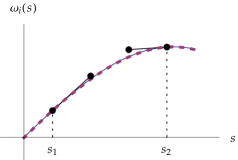
Figure 1. Schematic of interpolating a function using a cubic Bézier curve. The function to be interpolated is shown as a thin solid curve, and the constructed interpolating Bézier curve is shown by the heavy dashed curve. The large dots indicate the control points derived from the value and slope of the function at $s_{1}$ and $s_{2}$.

To treat the second source of error—arising from the fact that non-parallel rotations do not commute—we could do the same as for the first source of error: increase the number of orbital slices. That approach, however, seems unnecessarily expensive when we use very accurate, or exact, orbital integrators.

It turns out that the rotation vector $\vec{\Omega}$ varies across a slice in a sufficiently simple manner that we may interpolate it across a slice using piece-wise cubic polynomials, constructed as Bézier curves [15]. To use this technique, we compute, at the edge of each slice during the orbital integration, not only $\vec{\Omega}$, but also the derivatives of its three components. With that information, we construct a cubic interpolating polynomial with the correct slope at the end points; see figure 1 for a schematic illustration. For the $\vec{\Omega}$ variations that occur in our simulations, this approach yields very accurate interpolating functions. Moreover, the low cost of evaluating this interpolating polynomial makes it possible to take many spin steps per orbital slice.

The PWC computation of the spin precession in (37b) will converge with a sufficiently large number of steps. If convergence requires an excessive number of steps, the use of cubic Bézier curves can speed up the computation. What the Bézier approach does not do is increase the rate at which the computation converges. For that we must look elsewhere, and that is the topic of the next section.

4.3. Romberg quadratures for spin precession

As we have seen, the spin precession across a beamline element is not, in reality, piece-wise constant; rather, within an element it varies smoothly with $s$. More significantly, the integrators based on (37) exhibit second-order convergence (see section 5.2). This quadratic convergence suggests the use of some accelerating technique to cancel the errors. In particular, we have applied a Romberg approach [5, 53] to spin integration, and, as we show later in this paper, the improvement is dramatic.

Instead of computing the rotation vectors at the middle of each slice, we now, for this new approach, compute them at the edges of each slice. We then accumulate the spin precession as in (37). For the first and last edges, however, we use a half-step; i. e. we replace $\Delta s$ by $\Delta s/2$. This is akin to using the trapezoidal rule for integration [5, 35]. We do this using $N$ slices, with $N$ a multiple of some power of two.

During the orbital integration, we record the value of $\vec{\Omega}$ at the edge of each slice. Then by keeping every other $\vec{\Omega}$, or every fourth, or every eighth, etc., we can approximate the net spin precession using a range of additional step-sizes that are related to the original by powers of two. In other words, we compute for these different step sizes a net quaternion that represents the spin precession of a given particle across an element. We obtain thus the sequence of quaternions

(38) $$Q(h),\;Q(h/2),\;Q(h/2^{2}),\;Q(h/2^{3}),\;\dotsc,$$

where $h$ denotes the coarsest step size.

For example, when crossing an element using eight slices, we will compute a total of nine $\vec{\Omega}$s: $\vec{\Omega}_{0}$ at the beginning of the first slice, $\vec{\Omega}_{1}$ at the end of the first slice, on through $\vec{\Omega}_{8}$ at the end of the last slice. Now, assuming each slice has length $\Delta s$, we multiply the first and last of these by $\Delta s/2$, and all the others by $\Delta s$, to obtain the sequence

$$\frac{1}{2}\Delta s\,\vec{\Omega}_{0},\ \Delta s\,\vec{\Omega}_{1},\ \Delta s\,\vec{\Omega}_{2},\ \dotsc,\ \frac{1}{2}\Delta s\,\vec{\Omega}_{8}.$$

After constructing the quaternions that correspond to each of these nine precession vectors, we multiply them together to obtain a net quaternion that represents one approximation to the exact spin precession across this element. This is one of the entries in the sequence (38) above. To obtain the entry to its immediate left, we drop every other $\vec{\Omega}$ and compensate by doubling the step size; the sequence

$$\Delta s\,\vec{\Omega}_{0},\ 2\Delta s\,\vec{\Omega}_{2},\ \dotsc,\ \Delta s\,\vec{\Omega}_{8},$$

thus yields another—the next coarser—approximation to the spin precession across this element. And so on.

We then compute the Romberg limit: First define by

(39a) $$Q_{0k}=Q(h/2^{k})$$

the sequence of approximations in (38). Then use the rule

(39b) $$Q_{j+1,k}=\frac{4^{j+1}Q_{j,k}-Q_{j,k-1}}{4^{j+1}-1}$$

to construct the Romberg table:

(39c) $$\begin{array}[]{ccccccc}Q_{00}&&&&&&\\ Q_{01}&&Q_{11}&&&&\\ Q_{02}&&Q_{12}&&Q_{22}&&\\ Q_{03}&&Q_{13}&&Q_{23}&&Q_{33}.\end{array}$$

This table may have more or fewer rows than indicated here, but the number at the bottom right is the Romberg limit of the initial data given in the first column. We normalise the resulting quaternion at the end of each element.

When integrating a well-behaved function over a finite interval, the trapezoidal rule together with the Romberg limit performs remarkably well with modest computational effort. Its efficiency, however, derives from the structure of the error term seen in the Euler-Maclaurin summation formula [35, 53], and the manner in which the Romberg algorithm cancels those errors. Here, on the other hand, we have a product of quaternions, and hence no a priori reason to suspect that the above will actually work. We tried it for a lark.

4.4. Solenoid fringe

In the thin-pancake model discussed earlier for the solenoid fringe, there exists a well-defined limit of the fringe length $\varepsilon$ times the precession vector $\vec{\Omega}$, as $\varepsilon\rightarrow 0$. In that limit, a spin crossing a solenoid fringe experiences a net rotation given by the vector

(40) $$\vec{\omega}=\pm\frac{b_{0}/2}{(B\rho)_{\circ}P_{s}}\Bigl{[}(1+G\gamma)(X,\,Y,\,0)-G(\gamma-1)\frac{XP_{x}+YP_{y}}{P^{2}}m\gamma\vec{V}\Bigr{]},$$

where we choose the leading plus or minus for entrance or exit, respectively. Here the kinetic momentum vector $m\gamma\vec{V}$ is as given in (36), except that we must insert a factor of $\frac{1}{2}$ in front of $A_{x}$ and $A_{y}$. In a similar manner, $P_{s}$ denotes the square-root in (33), but with the same factor of $\frac{1}{2}$ inserted before $A_{x}$ and $A_{y}$. These factors of $\frac{1}{2}$ enter because in going to the limit of a zero-length fringe, we evaluate the field strength in the middle of that fringe region.

4.5. Dipole and multipole fringes

A particle’s spin also experiences a kick when crossing the fringe of a multipole magnet. This spin kick arises predominantly from the longitudinal field component in the fringe. In the limit of a thin fringe, and to lowest order in the dynamical variables, the spin kick caused by the fringe of a normal (i. e. not skew) $2m$-pole magnet of strength $b_{m}$ is given by the rotation vector

(41) $$\vec{\omega}_{m}=-\frac{\pm b_{m}}{(B\rho)_{\circ}}(1+G)\frac{r^{m}}{m}\sin(m\phi)\,\hat{z},$$

where we convert $r^{m}\sin(m\phi)$ to a function of $X$ and $Y$ using $(X+\mathrm{i}\mspace{2.0mu}Y)^{m}=r^{m}\mathrm{e}^{\mathrm{i}m\phi}.$ For a skew multipole, in (41) replace $\sin$ by $\cos$, and $b_{m}$ by $a_{m}$.

The above result (41) is appropriate for beams that cross a fringe roughly normal to the entrance or exit face of the magnet. When entering, or exiting, a rectangular bend, however, a particle typically sees the longitudinal field $B_{z}$ as having a significant component transverse to its velocity. As long as $P_{x}$ is not too large, one may account for this effect by simply adding an extra term to (41) to obtain the rotation vector

(42) $$\vec{\omega}_{\text{rb}}=\vec{\omega}_{1}+\frac{\pm b_{1}}{(B\rho)_{\circ}}G(\gamma-1)P_{x}\,\hat{x},$$

which describes the spin kick experienced by a particle crossing the fringe of a rectangular bend. Note the factor of $G\gamma$ in the second term: it is one good reason for not using rectangular bends in machines designed for polarized beams, particularly at high energy.

If one requires a higher order computation of the spin kick across a magnet fringe, it is possible to apply a procedure analogous to that used for orbital kicks across fringe fields in [22].

5. Performance of integrators

In this section, we examine the performance of the orbital and spin integrators described in the previous two sections. Our principal focus is on the integrators for spin. We examine the orbital integrators—much more briefly—with the goal of understanding their impact on spin integration.

For the orbital integrators, we examine their performance in a particular context: that of Brookhaven’s Relativistic Heavy Ion Collider (RHIC) [32] operating at approximately $250\text{\,}\mathrm{GeV}$, with the optics settings used before the beta squeeze. For the spin integrators, we examine their single-element performance, as well as their performance in the context of spin tracking for RHIC. In this context, we note that RHIC has two full Siberian snakes on opposite sides of the ring to flip the spins, with the snake angles set to $\pm$$$. These settings mean that for a perfectly aligned RHIC, the design orbit will have a spin-tune of exactly $\frac{1}{2}$ [7, 37]. Sextupoles are adjusted to set the chromaticities to $(\xi_{x},\xi_{y})=(0.70,0.74)$, and the spin rotators near the interaction points are turned off. The latter are needed only after the beta squeeze, when the counter-rotating RHIC beams are brought to collision, and the experiments require longitudinal polarization at the interaction point. For our simulations, then, the equilibrium polarization is roughly vertical throughout the ring.

5.1. Orbit integrators

For the simulations discussed here, we read a RHIC lattice description from a file in SXF format [31]. Which integrator to use for which elements is set in a separate ‘.apdf’ file (for Accelerator Propagator Description Format). When referring to the integrators, we use the acronym BK/MK, or sometimes just “bend-kick”, to mean the use of (10) for sector bends, together with (24) and (25) for quadrupoles. The Siberian snakes were modelled as thin elements: they are transparent to the orbital motion, and they act on the spin according to snake angles defined in an input file. In the simulations described here, we use a base number $n_{b}$ of slices for all dipoles and most quadrupoles. Then for the strongest quadrupoles, those in the interaction region, we use $4n_{b}$ slices.

5.1.1. Poincaré sections

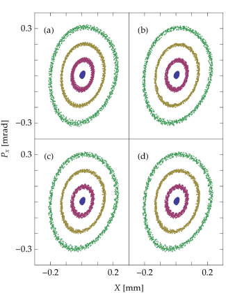
Figure 2. Poincaré sections for four sample particles using drift-kick integration with (a) $n_{b}=4$ and (b) $n_{b}=16$, and using BK/MK integration with (c) $n_{b}=1$ and (d) $n_{b}=16$.

To give a sense of how well the drift-kick and BK/MK integrators reproduce gross features of the orbital motion, we show Poincaré sections of the $X$-$P_{x}$ plane; see figure 2. The range of amplitudes shown is representative of beams at this azimuth in RHIC—the interaction point, before the beta squeeze is applied to the optics.

Figure 2 indicates that the drift-kick and BK/MK integrators produce the same gross features of the orbital motion. There are, however, differences in the details. In particular, the drift-kick traces with $n_{b}=4$ seem more elliptical, while the remaining traces seem more ovoid. The trace-widths also seem more regular for drift-kick integration with $n_{b}=4$, as compared to all the others. Differences between the two BK/MK integrators, with $n_{b}=1$ and $n_{b}=16$, are not visible with the bare eye. Differences between (b), (c), and (d) are much smaller than those between (a), on the one hand, and (c) and (d), on the other.

5.1.2. Orbital spectra and tune fitting

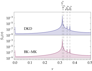
Figure 3. Spectrum of $X$ obtained using (a) drift-kick integration with $n_{b}=8$, or (b) BK/MK integration with $n_{b}=1$. The indicated tunes are all taken modulo 1.

In figure 3 we show the spectrum of $X$ obtained by taking a discrete Fourier transform of the $X$ coördinates obtained over the course of $T=1000$ turns,

(43) $$S_{X}(\nu)=\left|\frac{1}{T}\sum_{t=0}^{T}\mathrm{e}^{-\mathrm{i}2\pi t\nu}X(t)\right|^{2}.$$

The spectra were averaged over a bunch containing $N=1024$ particles with amplitudes typical for RHIC. The tunes marked in the figure (see top edge) are the design values for RHIC at this energy ($215.735\text{\,}\mathrm{GeV}$ kinetic): $\nu_{x}=28.6835$, $\nu_{y}=29.6742$. Note that we see peaks not only at $\nu_{x}$ and $\nu_{y}$, but also at $2\nu_{x}$ and $2\nu_{y}$—evidence of significant nonlinearity in the orbital motion.

As shown in figure 3, one can obtain a close match to the design orbital tunes using either drift-kick or BK/MK integration. However, in the case of drift-kick integration, one must adjust the strengths of the main quadrupoles by an amount that depends on the number of orbital slices used. No such adjustment is required when using BK/MK integration.

In the context of purely orbital tracking, adjusting the quadrupole strengths to fit the desired tunes is a sensible means of ensuring the correct linear behavior in accelerator simulations. In the context of spin tracking, however, such adjustments might be problematic, because changing a quadrupole’s strength changes the amount of spin precession a particle experiences as it crosses that element. In other words, fitting the orbital tune can perturb the integrated spin precession angle of a given particle—particularly at high energy, i. e., at large values of the naïve spin tune, $G\gamma$.

We can estimate the importance of this effect as follows. On crossing a quadrupole, a spin experiences a net precession with magnitude given approximately by $\omega=-(1+G\gamma)Ab_{2}L/(B\rho)_{\circ},$ where $A$ denotes the particle amplitude, and $L$ the quadrupole length. For the RHIC lattices we studied, the tune fitting required a relative change in $b_{2}$ that varied greatly with the step-size used for crossing the quadrupoles. For finely sliced lattices, the relative change in $b_{2}$ (from the value used for BK/MK integration) could be as small as a few times ${10}^{-5}$. At RHIC energies, this adjustment yields a sub-$\mathrm{\SIUnitSymbolMicro rad}$ change in the spin precession, and perhaps a few $\mathrm{\SIUnitSymbolMicro rad}$s over a full turn. As we shall see later, when one uses drift-kick orbital integration, this variation is negligible compared to other sources of error. On the other hand, for very coarse slicing, the relative change in $b_{2}$ can exceed $0.1\text{\,}\mathrm{\char 37\relax}$, which leads to a small, though noticeable, change in the simulated spin precession angle.

5.1.3. Single-turn errors

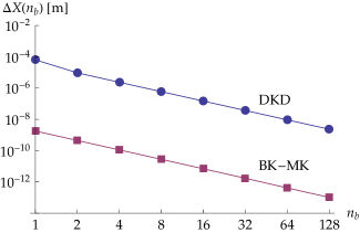
Figure 4. One-turn errors in $X$ versus $n_{b}$ for drift-kick integration (upper curve), and BK/MK integration (lower curve). The errors were computed by comparing with a data set produced using BK/MK integration and $n_{b}=256$.

For accurate spin tracking, it does not suffice to integrate the orbital motion in a manner that merely reproduces global properties of the phase-space distribution. Errors in particle orbits introduce errors in the spin rotations, possibly changing the character of the simulated spin dynamics. As a consequence, one must compute accurately the trajectories of individual particles.

To gain an understanding of the orbital errors on a per-particle basis, we look at the rms deviation between computed particle orbits and a reference solution for each particle. For the $X$ coördinate after $t$ turns, we thus compute

(44) $$\Delta X(t;n_{b})=\sqrt{\frac{1}{N}\sum_{\smash{j}=\smash{1}}^{N}\Bigl{[}X_{j}(t;n_{b})-X_{j}^{\text{(ref)}}(t)\Bigr{]}^{2}\,}\,.$$

The sum is over the particles in the bunch. The reference solution is computed with $n_{b}=128$ using the BK/MK integrators, i. e. $X_{j}^{\text{(ref)}}(t)=X_{j}(t;128)$.

Figure 4 shows the absolute error $\Delta X(1;n_{b})$ after one turn for a RHIC beam at approximately $216\text{\,}\mathrm{GeV}$ with a $95\text{\,}\mathrm{\char 37\relax}$ horizontal emittance $\varepsilon_{x}$ of $15\pi\text{\,}\mathrm{m}\mathrm{m}\,\mathrm{m}\mathrm{rad}$. The slope $-2$ on the $\log$-$\log$ scale shows that both drift-kick and BK/MK integrators exhibit second-order convergence in $s$. The drift-kick integrator starts out with a relative error of order one (cf. figure 2), indicating that with this very large step-size, the phases of the orbital motion are completely off: the errors are as large as they can be with a symplectic integrator. At $n_{b}=64$, the relative errors have decreased to about a part in ${10}^{4}$. On the other hand, the BK/MK integrators exhibit relative errors which start out below a part in ${10}^{6}$ and decrease until they are below about a part in ${10}^{9}$.

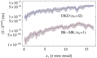
Figure 5. One-turn errors in $X$ versus amplitude for several different integrators: drift-kick with $n_{b}=32$ (upper curve), and BK/MK with $n_{b}=1$ (lower curve).

Figure 5 also shows one-turn errors in $X$, but here as a function of particle emittance. These results, which are consistent with those of figure 4, tell us that the accuracies of the different integrators have roughly the same amplitude dependence. To reduce the noise level in this graphic, we have averaged the results within non-overlapping bins that each contained $20$ particles in a narrow slice of emittance. The bands indicate one standard deviation above and below the computed average.

5.1.4. Evolution of orbital errors over many turns

Figure 6 shows the errors in the $X$ coördinate as a function of the number of turns for drift-kick integration and BK/MK integration. If we do not adjust the quadrupole strengths so as to fit the desired tunes, then the drift-kick integration errors oscillate periodically because of the tune errors. We see that behavior in the uppermost (tan) curve, for drift-kick integration with $n_{b}=8$. After fitting the tunes, we note that drift-kick integration errors with $n_{b}=4$ now track the minima of the tan oscillatory errors.

While the errors observed are much smaller for BK/MK integration—even with $n_{b}=1$—they always exhibit the same qualitative behavior: After a few hundred turns, even when using BK/MK integration, the errors grow approximately linearly because of unavoidable tiny differences in the tunes. We believe this is not a significant issue.

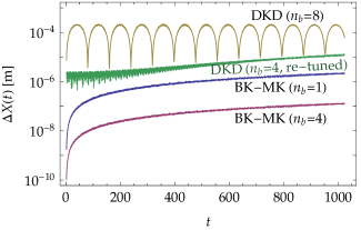
Figure 6. Evolution of the orbital error in $X$ as a function of turn number $t$. The four curves correspond to different methods of integration: from top to bottom they are drift-kick with $n_{b}=8$ and no tune fit (tan), drift-kick after tune fitting with $n_{b}=4$ (green), and BK/MK with $n_{b}=1$ (purple), and $4$ (maroon). For the reference solution, we used BK/MK with $n_{b}=16$.

5.2. Spin integrators

Here we describe the accuracy of our spin integrators. First, we discuss the errors seen when tracking across various individual beamline elements, where we focus on the impact of both step-size and Romberg iterations. We then discuss, more briefly, the spin integration errors seen over the course of a single turn and many turns.

5.2.1. Single-element errors

Figure 7. Absolute error in the computed spin versus the number of slices for a proton crossing several different beamline elements. All but the lower right graphic show results for a $200\text{\,}\mathrm{G}\mathrm{e}\mathrm{V}$ $p^{+}$ crossing a RHIC IR quad (top left), a RHIC arc dipole (top right), and a $2.1\text{\,}\mathrm{m}$, $1.3\text{\,}\mathrm{T}$ solenoid (bottom left). The bottom-right graphic shows the result for a $25\text{\,}\mathrm{G}\mathrm{e}\mathrm{V}$ $p^{+}$ traversing the same solenoid. Each curve corresponds to a different method of integrating the spin: PWC for piece-wise constant integration; the $k$ values indicate the number of Romberg iterations.

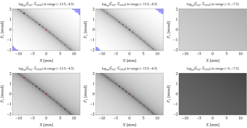
Figure 8. Absolute error in the computed spin across a RHIC dipole for a range of initial conditions in orbital phase space. Darker (lighter) grays represent smaller (larger) errors. Points outside the range indicated above each graphic are colored red if below, and blue if above. The error range covers the same five decades in the four graphics to the left. In the right-hand two graphics, the error range is again the same, but covers just a decade and a half that is mostly above the range in the other graphics. The upper and lower rows respectively show results obtained using PWC spin integration with four and eight slices. The three columns correspond to different values for $P_{y}^{i}$ and $P_{t}^{i}$: $P_{y}^{i}=0$, $P_{t}^{i}=0$ (left); $P_{y}^{i}=$20\text{\,}\mathrm{\SIUnitSymbolMicro rad}$$, $P_{t}^{i}=0$ (middle); $P_{y}^{i}=$20\text{\,}\mathrm{\SIUnitSymbolMicro rad}$$, $P_{t}^{i}\approx$0.35\text{\times}{10}^{-3}$$ (right).

The graphics in figure 7 show the spin integration errors we computed when tracking a particular particle across several different beamline elements. From top to bottom, those elements are a quadrupole, a sector bend, a solenoid, and another solenoid (but with a very low energy proton, such that the total spin rotation is comparable to $90\mathrm{°}$). In each of those graphics, the solid curve labelled PWC corresponds to piece-wise constant spin integration, where for the orbital motion we used the integrators given in sections 3.1, 3.3, and 3.7. In all cases the slope $-2$ reveals second-order convergence for PWC spin integration. The remaining curves correspond to $k$ Romberg iterations (i. e. $Q_{kk}$) applied to the PWC data obtained for the given number of slices. Since we do not know the result of exact spin integration, we have here estimated the spin integration error as the absolute difference between the result $\vec{\mathcal{S}}^{N}$ obtained using $N$ slices and what we considered our “best” result, $\vec{\mathcal{S}}_{\text{best}}$.

In figure 7, we have used for $\vec{\mathcal{S}}_{\text{best}}$ the results we obtained using $256$ slices and three Romberg iterations. If we instead use for $\vec{\mathcal{S}}_{\text{best}}$ our most finely sliced PWC result, then small details in these graphics change, but the overall implication holds—that one or more iterations of the Romberg procedure can dramatically reduce the errors made by PWC spin integration. In the case of the quadrupole integrated using four slices, we see that two Romberg iterations yield a four-decade reduction in the error—to a level that requires some four-hundred slices using just PWC spin integration. For the solenoid, a similar statement holds in the case of a low-energy proton; and in the high-energy case, one Romberg iteration suffices to reduce the spin integration error to the level of round-off. For the sector bend, we see a less dramatic absolute reduction in the error; but even there, between $8$ and $64$ slices, the slope $-4$ on the $k=1$ curve tells us that one Romberg iteration converts second-order PWC integration to fourth-order.

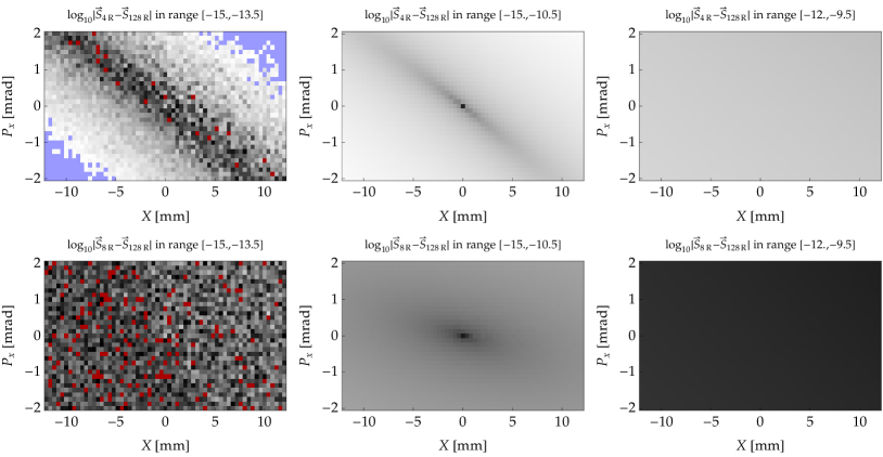
Figure 9. Absolute error in the computed spin across a RHIC dipole for a range of initial conditions in orbital phase space. Each of the graphics in this figure show results for the same orbital initial conditions and the same number of slices as the corresponding graphic in figure 8. The differences are that the integration here includes one Romberg step, and the error ranges are significantly lower.

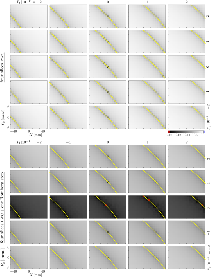
Figure 10. Absolute error in the computed spin using four slices across a RHIC dipole. Each small graphic covers a range of initial conditions in horizontal phase-space (see labels at lower left). The rows and columns correspond respectively to different initial values for $P_{y}$ and $P_{t}$ (see labels along right and top edges). For the lower set of graphics, we added one Romberg iteration.

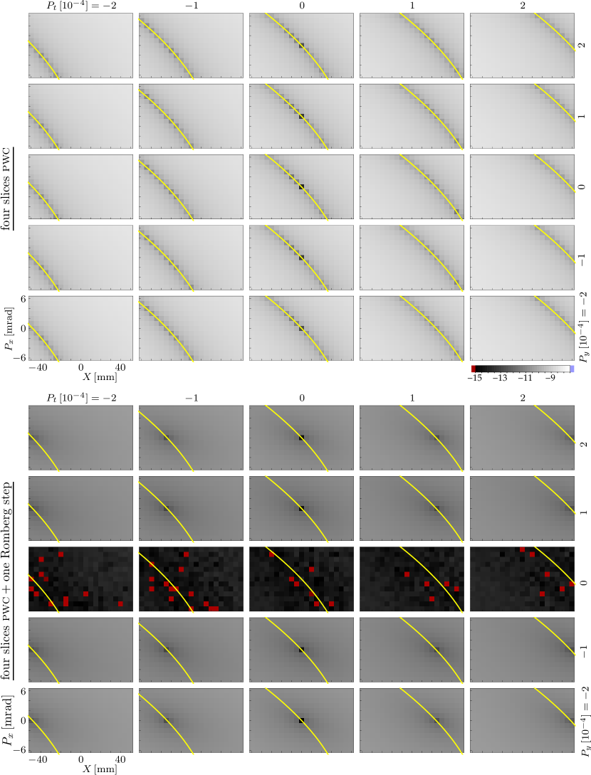
Figure 11. Absolute error in the computed spin using eight slices across a RHIC dipole for a range of initial conditions. See also the caption of figure 10. The two sets of twenty-five graphics correspond to PWC spin integration (upper set) and PWC plus one Romberg iteration (lower set).

The graphics in figure 7 illustrate the scaling of spin integration errors for one particular particle, and the impact of Romberg iterations on PWC spin integration. Were we just lucky, or do we see similar behavior across the relevant phase-space? The next several figures address this question, illustrating the effect of Romberg quadratures on spin integration for particles covering a range of initial conditions in phase-space.

For the sector bend, we examine spin integration errors across a RHIC dipole: a $9.45\text{\,}\mathrm{m}$ long magnet set to bend $200\text{\,}\mathrm{GeV}$ protons $2.225\mathrm{°}$, so with magnetic field strength $B\approx$2.75\text{\,}\mathrm{T}$$. As a proxy for exact tracking, we settled on, after considerable testing, one Romberg iteration applied to $128$ slices of PWC spin integration. Furthermore, because a magneto-static dipole is translationally invariant in both $Y$ and $T$, we examine how the spin integration errors vary with respect to just $X$, $P_{x}$, $P_{y}$, and $P_{t}$.

In figure 8, we show the absolute error in the computed spin using PWC spin integration with either four or eight slices (upper and lower rows, respectively). Figure 9 shows the corresponding results obtained after we apply one Romberg iteration. To help the reader make a proper comparison, we note further details in the captions of those two figures.

A comparison of figures 8 and 9 suggests that applying Romberg quadratures to spin integration across a sector bend does indeed reduce the error throughout phase-space. But we are also struck by some of the features seen in figure 8: the pronounced valley that runs diagonally across the four graphics on the left; and the much flatter and somewhat larger errors in the presence of an energy deviation, seen in the two graphics on the right.

To gain some understanding of these features, we examined a much larger range of phase space; a range that is, in fact un-physically large for an arc dipole in RHIC. Figures 10 and 11 show the results. Each of the one hundred small graphics in those two figures covers the same range of horizontal phase space: $\pm 5\text{\,}\mathrm{cm}$ in $X$, and $\pm 6\text{\,}\mathrm{mrad}$ in $P_{x}$. They are laid out in four matrices of twenty-five graphics each, where the columns correspond to five different values of $P_{t}^{i}$, evenly spaced in the range $\pm 2\text{\times}{10}^{-4}$; and the rows correspond to five different values of $P_{y}^{i}$, evenly spaced in the range $\pm 0.2\text{\,}\mathrm{mrad}$. (See the labels at the top and to the right of each matrix of graphics.) To obtain the graphics in figure 10, we used four slices of PWC spin integration for the upper set of twenty-five graphics, and four slices plus one Romberg iteration for the lower set. We obtained the data shown in figure 11 using eight slices. In all the graphics, the gray-scale covers the same (logarithmic) range of errors: from black at ${10}^{-15}$ to white at $e-7.5$.

The graphics shown in figures 10 and 11 reiterate the message that applying a Romberg step to the result of PWC spin integration can reduce the error throughout the phase-space of orbital initial conditions. In addition, however, we draw the reader’s attention to the yellow curve, overlaid on each graphic, which clearly follows the deep valley seen in those graphics for which no Romberg step was applied. In each graphic, this curve is the locus of points $(X^{i},P_{x}^{i})$ for which the value of $P_{x}$ at the magnet exit equals the value $P_{x}^{i}$ at the magnet entrance. This value is given by

(45) $$P_{x}^{\text{sym}}(X^{i})=\cos\Bigl{(}\frac{hL}{2}\Bigr{)}\biggl{[}\sqrt{1+\frac{2}{\smash{\beta_{\circ}}}P_{t}+P_{t}^{2}-P_{y}^{2}-(1+hX^{i})^{2}\cos^{2}\Bigl{(}\frac{hL}{2}\Bigr{)}}\\ -(1+hX^{i})\sin\Bigl{(}\frac{hL}{2}\Bigr{)}\bigg{]}.$$

Note that the dependence of $P_{x}^{\text{sym}}$ on $P_{y}$ and $P_{t}$ occurs only under the square-root, and that there it is linear in $P_{t}$ and quadratic in $P_{y}$. This difference (together with the fact that $P_{y}$ and $P_{t}$ denote small quantities) explains why the yellow curves in figures 10 and 11 show little dependence on $P_{y}$, but very sensitive dependence on $P_{t}$.

Earlier, when examining figure 8, we noted that the two right-hand graphics have much flatter and somewhat larger error profiles than appear in the left-hand four graphics. Now, on comparing with the graphics in figure 10, we see what happened: the valley simply moved “off stage” as we increased the energy deviation.

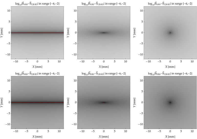
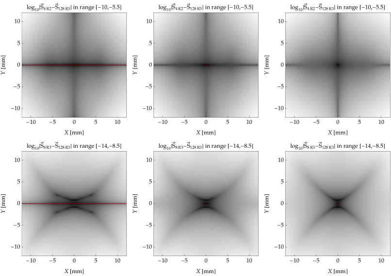
Figure 12. Absolute error in the computed spin across a RHIC IR quadrupole. The rows, from top to bottom, show results obtained using four slices, eight slices, four slices plus two Romberg steps, and eight slices plus three Romberg steps. The columns, from left to right, show results averaged over spins covering an opening angle about the vertical of $0\mathrm{°}$, $20\mathrm{°}$, and $180\mathrm{°}$.

For the quadrupole, we examine spin integration errors across a RHIC interaction region (IR) quadrupole: in this case a $1.83\text{\,}\mathrm{m}$ long magnet set to focus $200\text{\,}\mathrm{GeV}$ protons with a magnetic quadrupole gradient of $b_{2}=$70.0\text{\,}\mathrm{T}\text{\,}{\mathrm{m}}^{-1}$$. As a proxy for exact tracking, we settled on, again after much testing, three Romberg iterations applied to $128$ slices of PWC spin integration.

A coarse examination over the range of initial conditions $\pm 20\text{\,}\mathrm{mm}$ in $X$ and $Y$, $\pm 20\text{\,}\mathrm{\SIUnitSymbolMicro rad}$ in $P_{x}$ and $P_{y}$, and $\pm 0.35\text{\times}{10}^{-3}$ in $P_{t}$ indicate that (at least within this phase-space domain) spin integration errors change little with respect to variations in the transverse momenta $P_{x}$ and $P_{y}$, or the relative energy deviation $P_{t}$. As a consequence, here we show graphics of the spin integration errors for this element only in the $(X,Y)$ plane, with $P_{x}^{i}=P_{y}^{i}=P_{t}^{i}=0$.

In the case of the sector bend, the spin integration error does not appear to depend on the initial spin orientation. For the quadrupole, however, the accuracy of spin integration very definitely depends on the initial spin, so we have included that dependence in the results shown here.

In figure 12, we show the absolute error in the computed spin across a RHIC IR quadrupole. The first two rows show results obtained with PWC spin integration using either four slices (first row), or eight slices (second). The results shown in the lower two rows correspond to applying our Romberg procedure to the first two rows: four slices plus two Romberg steps (third row), or eight slices plus three Romberg steps (bottom row). As indicated above each graphic, the gray-scale in the first two rows covers the same (logarithmic) range of errors: from black at ${10}^{-6}$ to white at ${10}^{-2}$. In the third row, the range goes from ${10}^{-10}$ to $e-5.5$, which means most of the errors in the third row (all except small triangles in the corners) lie below the errors in the upper two rows. In the last row, the range of ${10}^{-14}$ to $e-8.5$ means the errors here lie entirely below those of the upper two rows; and they lie below most of the errors in the third row.

The columns in figure 12 correspond to averaging over various sets of initial spins. We generated a quasi-random distribution of spins (i. e., points on the unit sphere [44]) with opening angle $\alpha$ about the vertical: $\alpha=$$$ (left column), $20\mathrm{°}$ (middle), and $180\mathrm{°}$ (right).

In the case of a vertical spin ($\alpha=$$$), the errors vanish for orbital motion in the mid-plane because the vertical spin remains parallel to the vertical field everywhere along those orbits and therefore does not precess. What about other particles, those launched still with a vertical initial spin, but away from the mid-plane? For particles traversing a RHIC IR quad, the $\vec{\Omega}$ of (6b) lies predominantly along the quadrupole magnetic field, $(b_{2}Y,b_{2}X,0)$. Since the component of $\vec{\Omega}$ orthogonal to the spin is the component that rotates the spin, it follows that an initially vertical spin should be most sensitive to variations in $Y$, and rather insensitive to variations in $X$. This suggests why the two graphics in the upper left of figure 12—those for $\alpha=$$$ and no Romberg iterations—show essentially no variation with respect to $X^{i}$. Moreover, the fact that the orbital variation in $Y$ is (to first order) proportional to $Y^{i}$ suggests why the errors in those same two graphics increase away from the horizontal mid-plane.

As we allow the distribution of initial spins to open up ($\alpha>$$$), the distribution of errors (before the application of any Romberg iterations) quickly becomes more symmetric about the quadrupole axis. See the four graphics in the upper-right of figure 12. After we apply one or more Romberg steps, the quadrupole spin-integration errors become smaller and develop additional structure across the $(X,Y)$ plane. See the bottom two rows of figure 12. We do not yet understand the origin of this structure.

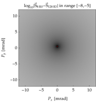
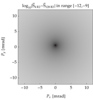
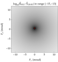
Figure 13. Absolute error in the computed spin across a solenoid. We computed the data shown in these three graphics using, from left to right, eight slices PWC spin integration, four slices PWC plus two Romberg iterations, and eight slices PWC plus three Romberg iterations. Note the different error ranges indicated above each graphic: with each step across the page, the errors fall by several decades.

For the solenoid, we examine spin integration errors across a $1.3\text{\,}\mathrm{T}$, $2.1\text{\,}\mathrm{m}$ long magnet. For the $200\text{\,}\mathrm{GeV}$ protons we used in previous elements, we find that four slices together with one or two levels of Romberg quadratures suffice to reduce errors to the level of round-off. In this case, however, the particle experiences very little spin rotation—of order $10\text{\,}\mathrm{mrad}$. We therefore chose to look at the spin integration errors for a much lower energy proton, $1.2\text{\,}\mathrm{GeV}$, traversing this same magnet. In this case the spin rotation is of order $0.6\text{\,}\mathrm{rad}$. As a proxy for exact tracking, we again settled on three Romberg iterations applied to $128$ slices of PWC spin integration.

Given the homogeneous nature of a solenoid’s body magnetic field in our thin-fringe approximation, we expect spin integration errors across this element to exhibit very little dependence on $X^{i}$, $Y^{i}$, or $P_{t}^{i}$. A coarse examination over a range of initial conditions in phase space indicates that this is indeed the case. As a consequence, here we show graphics of the spin integration errors for this element only in the $(P_{x},P_{y})$ plane.

In figure 13, we show the absolute error in the computed spin for a $1.2\text{\,}\mathrm{GeV}$ proton traversing the solenoid described above. The top graphic shows the result obtained using eight slices of PWC spin integration. The two graphics below show results obtained using four slices plus two Romberg steps (middle), and eight slices plus three Romberg steps (bottom). As indicated by the ranges noted above each graphic, the error ranges in these three graphics do not overlap. Indeed, the error range drops by several decades with each step down the page.

5.2.2. Single-turn errors

In this section, we examine spin integration errors after a full turn in the same RHIC lattice used for the orbital studies in section 5.1. See figures 14 and 15. As our measure of the error, we use the mean difference between the spin computed using a given set of numerical algorithms, and a reference solution that we use as a proxy for the exact result. The mean is taken over an ensemble of spins in a beam. We compute thus, at turn $t$,

(46) $$\Delta\vec{\mathcal{S}}(t)=\frac{1}{N}\sum_{j=1}^{N}\,\Bigl{|}\vec{\mathcal{S}}_{j}(t)-\vec{\mathcal{S}}_{j}^{\text{\,(ref)}}(t)\Bigr{|}\,.$$

For the results shown here, we computed the reference solution using BK/MK integration with $n_{b}=256$ and three Romberg iterations.

Figure 14 shows the absolute spin error as a function of the number of spin slices, here chosen identical to the number of orbital slices. No Romberg steps were applied, except when computing the reference solution. As a consequence, differences seen here between drift-kick results (upper two curves) and BK/MK results (lower curve) derive solely from differences in the orbital data passed to the Thomas-BMT equation.

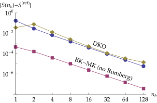
Figure 14. Single-turn spin errors as a function of the number of slices for several different integrators: drift-kick (blue circles, tan diamonds), and BK/MK (purple squares). The blue circles represent DKSKD: traverse each slice using half-drift, half-kick, spin rotation, half-kick, half-drift. The purple squares represent DKDSDKD: traverse each slice using half-DKD, spin rotation, half-DKD. The reference solution used BK/MK with $n_{b}=256$ together with three Romberg iterations.

At small numbers of orbital slices, spin integration based on drift-kick orbital integration reproduces only the one-turn spin-precession axis (close to the vertical). The precession angle about that axis, however, is completely off: compared to the reference solution, the phase of the spin precession is distributed uniformly over a $2\pi$ interval. Increasing the number of orbital slices improves the accuracy of spin integration, and at $n_{b}=64$ the single-turn spin-phase errors fall below a $\mathrm{mrad}$.

When performing spin integration based on BK/MK orbital integration, we obtain errors that are consistently two-and-a-half decades below those based on drift-kick integration (see the lowest curve in figure 14). This result, we emphasize, obtains in the absence of Romberg quadrature.

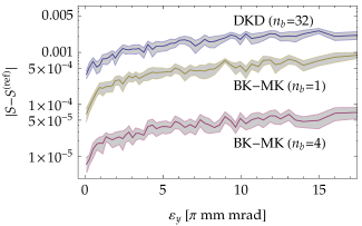
Figure 15. Amplitude dependence of the single-turn spin errors for three different integrators: drift-kick with $n_{b}=32$ (upper), and BK/MK with $n_{b}=1$ (middle), and $n_{b}=4$ (lower).

Figure 15 also shows the absolute spin error, but now as a function of particle emittance, after a single turn in the RHIC lattice. As in figure 14, no Romberg steps were applied—except in computing the reference solution—so that here also the differences seen derive solely from differences in the accuracy of the orbital integration. In addition, we have reduced the noise level in this graphic by, as in figure 5, averaging over narrow slices of emittance.

5.2.3. Evolution of spin errors

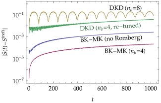
Figure 16. Accumulated spin error as a function of turn number, for multi-turn tracking in a RHIC lattice, using different methods of integration. From top to bottom: drift-kick integration with $n_{b}=8$ and no tune-fit (tan); the previous standard, a TEAPOT split with $n_{b}=4$ (green); BK/MK with $n_{b}=4$ and no Romberg (blue); and BK/MK with $n_{b}=4$ (purple). The simulated beam had a $95\text{\,}\mathrm{\char 37\relax}$ emittance of $15\pi\text{\,}\mathrm{m}\mathrm{m}\,\mathrm{m}\mathrm{rad}$.

We also examined how spin errors evolve over the course of many simulated turns in RHIC. In figure 16 we use the accumulated spin error to compare different methods of integration. The green curve shows results obtained using the previous standard: a TEAPOT split with four slices for most elements, but $16$ slices for the strong elements around the interaction regions. The lowest two curves we obtained using the new integrators, also with $n_{b}=4$. For the blue curve, we used just the “trapezoidal” rule (PWC of figure 7). For the lowest curve, we computed a Romberg limit using a maximum $k$ of $3$.

The topmost curve, obtained using drift-kick integration with $n_{b}=8$, but without retuning the lattice, exhibits pronounced oscillations. The tune errors in the orbital integration translate into these periodic oscillations of the spin errors.

6. GPU-accelerated implementation

In recent years, graphics processing units (GPUs) have emerged as an effective means to accelerate compute-intensive workloads. Because they are designed for massively data-parallel workloads with very regular control flow and memory access patterns, GPUs can dedicate a much larger fraction of their transistors to processing elements (registers and arithmetic and logic units) than can CPUs. As a consequence, they can achieve significantly larger computational throughput, performance per watt, and performance per dollar for workloads that are well-suited to their architecture. Particle tracking in the absence of space-charge effects is an embarrassingly parallel problem, and is therefore a natural fit for GPUs.

To map the spin-orbit tracking problem onto GPU hardware, we assign a GPU thread to each particle. For the actual tracking, we first transfer the state of a bunch to global memory on the GPU. This state comprises six-dimensional orbit data, three-dimensional spin data, plus the quaternions required for accumulating spin rotations. Particle tracking through individual beamline elements is broken up into several GPU kernels. We first compute the orbital motion through a particular beamline element. This requires loading orbit data at the element entrance from global memory into registers, computing the orbital motion using the integrators discussed in detail above, and then, at the element exit, writing the updated state back to global memory. During the orbital computation, we record in global memory the spin precession vector $\vec{\Omega}$ at the edge of each orbital slice. After integrating the orbital data through the given element, we then use the recorded $\vec{\Omega}$ data to update the quaternions using PWC spin integration plus one or more Romberg steps. We then update the spin.

The particle data resides on the GPU throughout spin-orbit tracking. By maintaining the data on the GPU, we avoid unnecessary data transfers between GPU and CPU, which can significantly slow down simulations. Particle data is occasionally copied back to the CPU in order to perform analysis; e. g., to compute (or update) the invariant spin field (ISF) at a particular location in the accelerator.

Figure 17. Time required to track $N$ particles through 100 turns of the RHIC lattice with GPU-accelerated integrators (solid). The CPU time (dashed) is an estimate; see text for details.

Figure 17 shows a comparison of the performance of spin-orbit tracking on a GPU and a CPU. The GPU simulations were carried out on the Dirac cluster at the National Energy Research Scientific Computing center (NERSC). The CPU performance is an estimate for an $8$-core CPU, based on the assumption that the simulation scales perfectly to $8$ CPU cores and that each CPU core is a factor $4$ faster than a GPU core. For up to a few hundred particles the CPU is faster than the GPU. For larger numbers of particles, the GPU accelerated simulations are faster. For a few ten-thousands of particles, the GPU accelerated simulations are approximately $15$ times faster than the corresponding CPU implementation.

7. Conclusion

In section 5.1, we showed that the BK/MK integrators can be much more efficient than the drift-kick integrators. This, of course, is well known (but see Forest’s discussion [23] for why drift-kick integration remains useful). Our purpose in including such a comparison here has to do with the influence of accurate orbit integration on the acccuracy of spin integration.

Figure 14 tells us that better orbit data yields more accurate spin integration. Using BK/MK integration yields a two-decade reduction of the spin errors as compared to drift-kick integration. We see that the improvement with the number of orbital slices is, in large part, due to the improvement in the orbital accuracy. In other words, with drift-kick integration the accuracy of the spin motion will improve just by increasing the number of orbital slices while holding the number of spin integration steps fixed.

On the other hand, for BK/MK integration, the discretization of the spin motion appears to be a significant source of error: A comparison of figures 4 and 5 with figures 14 and 15 show that the relative error in the orbital motion is much smaller than that in the spin rotation angle.

In section 4.2 we discussed interpolating the spin precession vectors, using cubic Bézier polynomials, as a means of rapidly computing multiple spin steps per orbital slice. To compute a Bézier curve for $\vec{\Omega}$, one must first determine the associated control points (see figure 1), and doing so requires computing the longitudinal derivative of $\vec{\Omega}$ at the beginning and end of each slice. For most elements, this is a non-trivial, hence time-consuming, computation. In other words, if we wish to enjoy the fast computation of many $\vec{\Omega}$ s along an interpolating Bézier curve, we must first invest some time computing $\vec{\Omega}^{\prime}$. As a trade-off, this means we benefit only if we plan to interpolate $\vec{\Omega}$ at some (possibly large) number of intermediate locations.

In the bargain, however, we do not improve the rate at which spin integration converges: The accuracy of this approach cannot improve upon what we obtain by taking smaller steps (i. e., using more orbital slices). In other words, the best we might hope for from interpolating the precession vector $\vec{\Omega}$, is a faster computation of PWC spin integration, which exhibits just second-order convergence.

As shown in figure 7, as well as in figures 8 through 13, the application of Romberg quadratures to PWC spin integration does increase the rate of convergence. Moreover, this approach requires only a modest number of orbital slices. Applying the Romberg algorithm to a sequence of quaternion products constitutes an easy and fast means of accelerating the convergence of spin integration. As a consequence, we have not pursued further the use of Bézier curves to speed up the computation of $\vec{\Omega}$.

Note that our initial motivation for using quaternions was the factor of two savings in arithmetic they convey. After discovering that Romberg applied to quaternions accelerates the convergence of the spin motion, we have another—much more significant—reason to use quaternions when integrating the Thomas-BMT equation for spin motion.

Concerning the convergence of spin motion, we here comment on what happens when simulating a system near a spin-orbit resonance [9]. First, note that in such a system a particle’s spin orientation becomes very sensitive to even very tiny perturbations. As a consequence, if we follow a single spin and ask for it’s motion to converge as we slice the lattice ever more finely, we may never see that happen. As with the orbital motion, we do not—cannot—ask for the “exact result”, because the machine we build is not the one we designed (though we hope it is close!). We instead ask for accurate qualitative dynamics, as revealed by phase-space portraits.

Second, note that the integrators are particular to given elements. In other words, they care only about the mapping of phase-space coördinates across a single element: $z^{i}\text{ at entrance}\rightarrow z^{f}\text{ at exit}$. On the other hand, a resonance condition can exist only in a ring: it is defined by the ring. One might therefore expect that the choice of integrator is, in some sense, independent of the proximity and strength of a resonance. But this expectation can hold only if the integrators are independent of, or have no effect on, whatever properties define the resonance.

When using drift-kick integrators, we know the tune seen in tracking data depends on how finely we slice our elements. What happens, then, as we approach a resonance? If we increase the slicing so as to ensure convergence, the effective tune changes. Hence the distance to resonance changes, and the spin dynamics can appear quite different—especially because of its sensitivity in the neighborhood of a resonance. If, on increasing the slicing we also re-tune the lattice, then the distance to resonance, as defined by the orbital tunes, remains the same. But the quadrupole strengths do change, and this implies a change in the spin tune for a given simulated particle [9]. And so again the distance to resonance changes, and again the spin dynamics can appear quite different because of its sensitivity in the neighborhood of a resonance.

Because BK/MK integrators yield the same linear orbital tunes independently of slicing, they are not subject to the same difficulties.

In addition to the improved accuracy and accelerated convergence of spin tracking, our code benefits from the significant speed-up it derives just from its implementation on GPUs. As shown in figure 17, a reasonable estimate for that benefit yields a speed-up factor of about 15. On a more practical level, we note that on one of NVIDIA’s GeForce TITAN GPU nodes, computing an ISF for RHIC at ${10}^{4}$ phase-space locations using ${10}^{3}$ turns takes less than fifteen minutes.

Finally, we are currently implementing integrators for other types of optical elements. These include electrostatic lenses, which are important for simulating EDM experiments, as well as better models for Siberian snakes.

References

- Abell et al. [2013] D. T. Abell, D. Meiser, D. P. Barber, M. Bai, and V. H. Ranjbar. GPU-accelerated dynamics and analysis for RHIC. In Petit-Jean-Genaz et al. [52], pages 1037–1039. URL http://accelconf.web.cern.ch/accelconf/ipac2013/papers/mopwo066.pdf.
- Abelleira Fernandez et al. [2012] J. L. Abelleira Fernandez, C. Adolphsen, A. N. Akay, et al. A Large Hadron electron Collider at CERN: Report on the physics and design concepts for machine and detector. Eprint http://arxiv.org/abs/1206.2913, Sept. 2012.
- Abeyratne et al. [2012] S. Abeyratne, A. Accardi, S. Ahmed, et al. Science requirements and conceptual design for a polarized medium energy electron-ion collider at Jefferson Lab. Eprint http://arxiv.org/abs/1209.0757, Sept. 2012.
- Accardi et al. [2011] A. Accardi, V. Guzey, A. Prokudin, and C. Weiss. Nuclear physics with a medium-energy Electron-Ion Collider. Eprint http://arxiv.org/abs/1110.1031, Oct. 2011.
- Acton [1996] F. S. Acton. Real Computing Made Real: Preventing Errors in Scientific and Engineering Calculations. Princeton University Press, Princeton, NJ, 1996.
- Aidala et al. [2013] C. A. Aidala, S. D. Bass, D. Hasch, and G. K. Mallot. The spin structure of the nucleon. Rev. Modern Phys., 85(2):655–691, Apr.–June 2013. doi: 10.1103/RevModPhys.85.655.
- Bai [2008] M. Bai. RHIC polarized proton status and plan. Eur. Phys. J. Special Topics, 162:181–189, Aug. 2008. doi: 10.1140/epjst/e2008-00793-8.
- Balandin and Golubeva [1997] V. V. Balandin and N. I. Golubeva. Hamiltonian methods for the study of polarized proton beam dynamics in accelerators and storage rings. In J. J. Bisognano and A. A. Mondelli, editors, Computational accelerator physics, volume 391 of AIP Conference Proceedings, Woodbury, NY, Mar. 1997. AIP Press. See also http://arxiv.org/abs/physics/9903032.
- Barber et al. [2004] D. P. Barber, J. A. Ellison, and K. Heinemann. Quasiperiodic spin-orbit motion and spin tunes in storage rings. Phys. Rev. ST Accel. Beams, 7(12):124002, Dec. 2004. doi: 10.1103/PhysRevSTAB.7.124002. An extended version is available at http://arxiv.org/abs/physics/0412157.
- Bargmann et al. [1959] V. Bargmann, L. Michel, and V. L. Telegdi. Precession of the polarization of particles moving in a homogeneous electromagnetic field. Phys. Rev. Lett., 2(10):435–436, May 1959. doi: 10.1103/PhysRevLett.2.435.
- [11] M. Berz. COSY-Infinity. http://cosyinfinity.org.
- Biedenharn and Louck [1981] L. C. Biedenharn and J. D. Louck. Angular Momentum in Quantum Physics: Theory and Applications, volume 8 of Encyclopedia of Mathematics and its Applications. Addison-Wesley Publishing Co., Reading, MA, 1981.
- Brown [1982] K. L. Brown. A first- and second-order matrix theory for the design of beam transport systems and charged particle spectrometers. SLAC Report 75, Stanford Linear Accelerator Center, Stanford, CA, June 1982. URL http://www.slac.stanford.edu/pubs/slacreports/slac-r-075.html.
- Brüning and Klein [2013] O. Brüning and M. Klein. The Large Hadron electron Collider. Eprint http://arxiv.org/abs/1305.2090, May 2013.
- Casselman [2005] B. Casselman. Mathematical Illustrations: A Manual of Geometry and PostScript. Cambridge University Press, Cambridge, UK, 2005.
- Chao [1981] A. W. Chao. Evaluation of radiative spin polarization in an electron storage ring. Nucl. Instrum. Methods, 180(1):29–36, Feb. 1981. doi: 10.1016/0029-554X(81)90006-9. Also available as SLAC-PUB-2564.
- Dragt [1982] A. J. Dragt. Lectures on nonlinear orbit dynamics. In R. A. Carrigan, F. R. Huson, and M. Month, editors, Physics of High Energy Particle Accelerators: Fermilab Summer School, Batavia, IL, 13–24 July, 1981, volume 87 of AIP Conference Proceedings, pages 147–313, Woodbury, NY, 1982. AIP Press. doi: 10.1063/1.33615.
- Dragt [2015] A. J. Dragt. Lie Methods for Nonlinear Dynamics with Applications to Accelerator Physics. Jan. 2015. Latest version available at http://www.physics.umd.edu/dsat/.
- Dragt and Forest [1983] A. J. Dragt and É. Forest. Computation of nonlinear behavior of Hamiltonian systems using Lie algebraic methods. J. Math. Phys., 24(12):2734–2744, Dec. 1983. doi: 10.1063/1.525671.
- Eur [2002] MAD—Methodical Accelerator Design: User’s Guide. European Organization for Nuclear Research, Geneva, 2002. URL http://madx.web.cern.ch/madx/doc/madx_manual.pdf.
- Fischer and Bazilevsky [2012] W. Fischer and A. Bazilevsky. Impact of three-dimensional polarization profiles on spin-dependent measurements in colliding beam experiments. Phys. Rev. ST Accel. Beams, 15(4):041001, Apr. 2012. doi: 10.1103/PhysRevSTAB.15.041001.
- Forest [1998] É. Forest. Beam Dynamics: A New Attitude and Framework, volume 8 of The Physics and Technology of Particle and Photon Beams. Harwood Academic Publishers, Amsterdam, 1998.
- Forest [2006] É. Forest. Geometric integration for particle accelerators. J. Phys. A: Math. Gen., 39(19):5321–5377, May 2006. doi: 10.1088/0305-4470/39/19/S03.
- Forest [2010] É. Forest. Orbital and spin normal forms in FPP or Propaganda in mathematical physics. KEK Report 2010-39, KEK, Tsukuba, Japan, Nov. 2010. URL http://www-lib.kek.jp/cgi-bin/kiss_prepri.v8?KN=201027039&OF=8.
- Forest and Milutinović [1988] É. Forest and J. Milutinović. Leading order hard edge fringe fields effects exact in and consistent with Maxwell’s equations for rectilinear magnets. Nucl. Instrum. Methods Phys. Res., Sect. A, 269(3):474–482, June 1988. doi: 10.1016/0168-9002(88)90123-4.
- Forest et al. [1994] É. Forest, M. F. Reusch, D. L. Bruhwiler, and A. Amiry. The correct local description for tracking in rings. Part. Accel., 45:65–94, 1994.
- Forest et al. [2002] É. Forest, F. Schmidt, and E. McIntosh. Introduction to the Polymorphic Tracking Code. KEK Report 2002-3, KEK, Tsukuba, Japan, 2002. URL http://www-lib.kek.jp/cgi-bin/kiss_prepri.v8?KN=200302020&OF=4.
- Forest et al. [2006a] É. Forest, S. C. Leemann, and F. Schmidt. Fringe effects in MAD, Part I: Second-order fringe in MAD-X for the module PTC. KEK Report 2005-109, KEK, Tsukuba, Japan, Mar. 2006a. URL http://www-lib.kek.jp/cgi-bin/kiss_prepri.v8?KN=200527109&OF=8.
- Forest et al. [2006b] É. Forest, S. C. Leemann, and F. Schmidt. Fringe effects in MAD, Part II: Bend curvature in MAD-X for the module PTC. KEK Report 2005-110, KEK, Tsukuba, Japan, Mar. 2006b. URL http://www-lib.kek.jp/cgi-bin/kiss_prepri.v8?KN=200527110&OF=8.
- Forest et al. [2006c] É. Forest, Y. Nogiwa, and F. Schmidt. The FPP and PTC libraries. In Proceedings of the 9th International Computational Accelerator Physics Conference, Chamonix, France, 2–6 October 2006, pages 17–21, 2006c. URL http://accelconf.web.cern.ch/accelconf/icap06/papers/mom1mp02.pdf.
- Gröte et al. [1998] H. Gröte, J. Holt, N. Malitsky, F. Pilat, R. Talman, and C. G. Trahern. SXF (Standard eXchange Format): definition, syntax, examples. Technical Report RHIC/AP/155, Brookhaven National Laboratory, Upton, NY, Aug. 1998.
- Harrison et al. [2002] M. Harrison, S. G. Peggs, and T. Roser. The RHIC accelerator. Annu. Rev. Nucl. Part. Sci., 52:425–469, Dec. 2002. doi: 10.1146/annurev.nucl.52.050102.090650.
- Heinemann [1996] K. Heinemann. On Stern-Gerlach forces allowed by special relativity and the special case of the classical spinning particle of Derbenev-Kondratenko. Technical Report DESY-96-229, Deutsches Elektronen-Synchrotron, Hamburg, Germany, Nov. 1996. Available at http://arXiv.org/abs/physics/9611001.
- Heinemann and Hoffstätter [1996] K. Heinemann and G. H. Hoffstätter. Tracking algorithm for the stable spin polarization field in storage rings using stroboscopic averaging. Phys. Rev. E, 54(4):4240–4255, Oct. 1996. doi: 10.1103/PhysRevE.54.4240.
- Hildebrand [1987] F. B. Hildebrand. Introduction to Numerical Analysis. Dover Publications, Inc., Mineola, NY, second edition, 1987. Unabridged, slightly corrected republication of the second edition (1974) of the work first published by McGraw-Hill, Inc., in 1956.
- Hoffstaetter [2006] G. H. Hoffstaetter. High-Energy Polarized Proton Beams: A Modern View, volume 218 of Springer Tracts in Modern Physics. Springer, New York, NY, 2006.
- Huang et al. [2011] H. Huang, L. Ahrens, I. G. Alekseev, E. Aschnauer, et al. RHIC polarized proton operation and highlights. In C. Petit-Jean-Genaz, A. Blanco, I. Etxebarria, F. Perez, A. Wolski, and V. Schaa, editors, Proceedings of the 2nd International Particle Accelerator Conference, San Sebastian, Spain, 4–9 September 2011, pages 1888–1890, 2011. URL http://accelconf.web.cern.ch/accelconf/ipac2011/papers/tupz035.pdf.
- Lehrach [2012] A. Lehrach. Project overview and computational needs to measure electric dipole moments at storage rings. In D. Hecht, editor, Proceedings of the 11th International Computational Accelerator Physics Conference, Rostock, Germany, 19–24 August 2012, pages 7–11, 2012. URL http://accelconf.web.cern.ch/accelconf/icap2012/papers/moaai1.pdf.
- Luccio [1995] A. U. Luccio. Numerical spin tracking in a synchrotron computer code: SPINK—Examples (RHIC). Technical Report BNL-52481, Brookhaven National Laboratory, Upton, NY, Sept. 1995.
- Luccio and MacKay [1999] A. U. Luccio and W. W. MacKay, editors. Proceedings of the 1999 Particle Accelerator Conference, New York, NY, 29 March–2 April 1999, Piscataway, NJ, 1999. IEEE.
- Luccio et al. [1999] A. U. Luccio, A. Lehrach, J. Niederer, T. Roser, M. J. Syphers, and N. Tsoupas. New capabilities of the spin tracking code SPINK. In Luccio and MacKay [40]. URL http://accelconf.web.cern.ch/accelconf/p99/papers/tup44.pdf.
- Malitsky et al. [2003] N. Malitsky, R. Talman, M. Blaskiewicz, R. Calaga, R. Fliller III, A. Luccio, T. Satogata, and J. Wei. Towards the UAL open source project. In J. T. Chew, P. W. Lucas, and S. Webber, editors, Proceedings of the 2003 Particle Accelerator Conference, Portland, OR, 12–16 May 2003, page 272, Piscataway, NJ, 2003. IEEE. URL http://accelconf.web.cern.ch/accelconf/p03/papers/topb004.pdf.
- Mane [2012] S. R. Mane. Calculation of higher order nonradiative spin resonance strengths in circular accelerators. Nucl. Instrum. Methods Phys. Res., Sect. A, 680:35–42, May 2012. doi: 10.1016/j.nima.2012.04.024.
- Marsaglia [1972] G. Marsaglia. Choosing a point from the surface of a sphere. Ann. Math. Statist., 43(2):645–646, 1972. doi: 10.1214/aoms/1177692644.
- McLachlan and Quispel [2002] R. I. McLachlan and G. R. W. Quispel. Splitting methods. Acta Numer., 11:341–434, Jan. 2002. doi: 10.1017/S0962492902000053.
- [46] F. Méot. Zgoubi. http://sourceforge.net/projects/zgoubi/.
- Méot [1992] F. Méot. A numerical method for combined spin tracking and ray tracing of charged particles. Nucl. Instrum. Methods Phys. Res., Sect. A, 313(3):492–500, Mar. 1992. doi: 10.1016/0168-9002(92)90829-S.
- Miller et al. [2007] J. P. Miller, E. de Rafael, and B. L. Roberts. Muon : experiment and theory. Rep. Progr. Phys., 70(5):795–881, May 2007. doi: 10.1088/0034-4885/70/5/R03.
- Mitchell and Dragt [2010] C. E. Mitchell and A. J. Dragt. Accurate transfer maps for realistic beamline elements: Straight elements. Phys. Rev. ST Accel. Beams, 13(6):064001, June 2010. doi: 10.1103/PhysRevSTAB.13.064001.
- Onderwater [2011] C. J. G. Onderwater. Search for EDMs using storage rings. J. Phys.: Conf. Ser., 295:012008, 2011. doi: 10.1088/1742-6596/295/1/012008.
- Papaphilipou and Abell [2000] Y. Papaphilipou and D. T. Abell. Beam dynamics analysis and correction of magnet field imperfections in the SNS accumulator ring. In A. Gallo, editor, Proceedings of the 7th European Particle Accelerator Conference, Vienna, Austria, 26–30 June 2000, pages 1453–1455, Geneva, 2000. European Physical Society. URL http://accelconf.web.cern.ch/accelconf/e00/papers/mop6a01.pdf.
- Petit-Jean-Genaz et al. [2013] C. Petit-Jean-Genaz et al., editors. Proceedings of the 4th International Particle Accelerator Conference, Shanghai, China, 12–17 May 2013, 2013.
- Press et al. [2002] W. H. Press, S. A. Teukolsky, W. T. Vetterling, and B. P. Flannery. Numerical Recipes in C++: The Art of Scientific Computing. Cambridge University Press, Cambridge, UK, second edition, 2002.
- Ranjbar et al. [2011] V. H. Ranjbar, F. Méot, and M. Bai. Spin tracking with GPUs to 250 GeV in RHIC lattice. In T. Satogata, editor, Proceedings of the 2011 Particle Accelerator Conference, New York, NY, 28 March–1 April 2011, pages 1624–1626, Piscataway, NJ, 2011. IEEE. URL http://accelconf.web.cern.ch/accelconf/pac2011/papers/wep080.pdf.
- Roberts [2010] B. L. Roberts. Status of the Fermilab muon experiment. Eprint http://arxiv.org/abs/1001.2898v2, Jan. 2010.
- [56] D. Sagan. Bmad. http://www.lns.cornell.edu/~dcs/bmad/.
- Schachinger and Talman [1985] L. Schachinger and R. Talman. TEAPOT: A thin element accelerator program for optics and tracking. Technical Report SSC-52, SSC Central Design Group, Dec. 1985. URL http://lss.fnal.gov/archive/other/ssc/ssc-52.pdf.
- Thomas [1927] L. H. Thomas. The kinematics of an electron with an axis. Philos. Mag. S 7, 3(13):1–22, Jan. 1927. doi: 10.1080/14786440108564170.
- Venturini and Dragt [1999a] M. Venturini and A. J. Dragt. Accurate computation of transfer maps from magnetic field data. Nucl. Instrum. Methods Phys. Res., Sect. A, 427(1–2):387–392, May 1999a. doi: 10.1016/S0168-9002(98)01518-6.
- Venturini and Dragt [1999b] M. Venturini and A. J. Dragt. Computing transfer maps from magnetic field data. In Luccio and MacKay [40], pages 1593–1595. URL http://accelconf.web.cern.ch/accelconf/p99/papers/tup50.pdf.
- Vogt [2000] M. Vogt. Bounds on the Maximum Attainable Equilibrium Polarization of Protons at High Energy in HERA. PhD dissertation, Universität Hamburg, 2000.
- Yoshida [1990] H. Yoshida. Construction of higher order symplectic integrators. Phys. Lett. A, 150(5–7):262–268, Nov. 1990. doi: 10.1016/0375-9601(90)90092-3.