A TB-HIV/AIDS coinfection model and optimal control treatment

Abstract.

We propose a population model for TB-HIV/AIDS coinfection transmission dynamics, which considers antiretroviral therapy for HIV infection and treatments for latent and active tuberculosis. The HIV-only and TB-only sub-models are analyzed separately, as well as the TB-HIV/AIDS full model. The respective basic reproduction numbers are computed, equilibria and stability are studied. Optimal control theory is applied to the TB-HIV/AIDS model and optimal treatment strategies for co-infected individuals with HIV and TB are derived. Numerical simulations to the optimal control problem show that non intuitive measures can lead to the reduction of the number of individuals with active TB and AIDS.

Cristiana J. Silva and Delfim F. M. Torres

Center for Research and Development in Mathematics and Applications (CIDMA)

Department of Mathematics, University of Aveiro, 3810–193 Aveiro, Portugal

1. Introduction

According with the World Health Organization (WHO), the human immunodeficiency virus (HIV) and mycobacterium tuberculosis are the first and second cause of death from a single infectious agent, respectively [48]. Acquired immunodeficiency syndrome (AIDS) is a disease of the human immune system caused by infection with HIV. HIV is transmitted primarily via unprotected sexual intercourse, contaminated blood transfusions, hypodermic needles, and from mother to child during pregnancy, delivery, or breastfeeding [37]. There is no cure or vaccine to AIDS. However, antiretroviral (ART) treatment improves health, prolongs life, and substantially reduces the risk of HIV transmission. In both high-income and low-income countries, the life expectancy of patients infected with HIV who have access to ART is now measured in decades, and might approach that of uninfected populations in patients who receive an optimum treatment (see [12] and references cited therein). However, ART treatment still presents substantial limitations: does not fully restore health; treatment is associated with side effects; the medications are expensive; and is not curative. Following UNAIDS global report on AIDS epidemic 2013 [45], globally, an estimated 35.3 million people were living with HIV in 2012. An increase from previous years, as more people are receiving ART. There were approximately 2.3 million new HIV infections globally, showing a 33% decline in the number of new infections with respect to 2001. At the same time, the number of AIDS deaths is also declining with around 1.6 million AIDS deaths in 2012, down from about 2.3 million in 2005.

Mycobacterium tuberculosis is the cause of most occurrences of tuberculosis (TB) and is usually acquired via airborne infection from someone who has active TB. It typically affects the lungs (pulmonary TB) but can affect other sites as well (extrapulmonary TB). In 2012, approximately 8.6 million people fell ill with TB and 1.3 million people died from TB. Nevertheless, TB death rate dropped 45 per cent between 1990 and 2012, and 22 million lives were saved through use of strategies recommended by WHO [48].

Individuals infected with HIV are more likely to develop TB disease because of their immunodeficiency, and HIV infection is the most powerful risk factor for progression from TB infection to disease [18]. In 2012, 1.1 million of 8.6 million people who developed TB worldwide were HIV-positive. The number of people dying from HIV-associated to TB has been falling since 2003. However, there were still 320 000 deaths from HIV-associated to TB in 2012, and further efforts are needed to reduce this burden [48]. ART is a critical intervention for reducing the risk of TB morbidity and mortality among people living with HIV and, when combined with TB preventive therapy, it can have a significant impact on TB prevention [48].

Collaborative TB/HIV activities (including HIV testing, ART therapy and TB preventive measures) are crucial for the reduction of TB-HIV coinfected individuals. WHO estimates that these collaborative activities prevented 1.3 million people from dying, from 2005 to 2012. However, significant challenges remain: the reduction of tuberculosis related deaths among people living with HIV has slowed in recent years; the ART therapy is not being delivered to TB-HIV coinfected patients in the majority of the countries with the largest number of TB/HIV patients; the pace of treatment scale-up for TB/HIV patients has slowed; less than half of notified TB patients were tested for HIV in 2012; and only a small fraction of TB/HIV infected individuals received TB preventive therapy [45].

The study of the joint dynamics of TB and HIV present formidable mathematical challenges due to the fact that the models of transmission are quite distinct [36]. Some mathematical models have been proposed for TB-HIV coinfection (see, e.g., [2, 3, 22, 28, 30, 36, 40]). In this paper, we propose a new population model for TB-HIV/AIDS coinfection transmission dynamics, where TB, HIV and TB-HIV infected individuals have access to respective disease treatment, and single HIV-infected and TB-HIV co-infected individuals under HIV and TB/HIV treatment, respectively, stay in a chronic stage of the HIV infection.

Optimal control is a branch of mathematics developed to find optimal ways to control a dynamic system [10, 16, 31]. While the usefulness of optimal control theory in epidemiology is nowadays well recognized (see, e.g., [4, 26, 27, 33, 34]), and has been applied to TB models (see, e.g., [5, 15, 19, 21, 41, 42]) and HIV models (see, e.g., [23, 29]), to our knowledge optimal control have never been applied to a TB-HIV/AIDS coinfection model. In this paper, we apply optimal control theory to our TB-HIV/AIDS model and study optimal strategies for the minimization of the number of individuals with TB and AIDS active diseases, taking into account the costs associated to the proposed control measures.

The paper is organized as follows. The model is formulated in Section 2. The HIV-only and TB-only sub-models of the full TB-HIV/AIDS model are analyzed in Section 3 and the full TB-HIV/AIDS model is analyzed in Section 4. In Section 5 we propose an optimal control problem and apply the Pontryagin maximum principle to derive its solution. In Section 6 numerical simulations and discussion of the results are carried out for the optimal control problem associated to the TB-HIV/AIDS model. We end mentioning some possible future work in Section 7.

2. Model formulation and basic properties

The model subdivides the human population into eleven mutually-exclusive compartments, namely susceptible individuals ($S$), TB-latently infected individuals, who have no symptoms of TB disease and are not infectious ($L_{T}$), TB-infected individuals, who have active TB disease and are infectious ($I_{T}$), TB-recovered individuals ($R$), HIV-infected individuals with no clinical symptoms of AIDS ($I_{H}$), HIV-infected individuals under treatment for HIV infection ($C_{H}$), HIV-infected individuals with AIDS clinical symptoms ($A$), TB-latent individuals co-infected with HIV (pre-AIDS) ($L_{TH}$), HIV-infected individuals (pre-AIDS) co-infected with active TB disease ($I_{TH}$), TB-recovered individuals with HIV-infection without AIDS symptoms ($R_{H}$), HIV-infected individuals with AIDS symptoms co-infected with active TB ($A_{T}$). The total population at time $t$, denoted by $N(t)$, is given by

$$N(t)=S(t)+L_{T}(t)+I_{T}(t)+R(t)+I_{H}(t)+C_{H}(t)+A(t)\\ +I_{TH}(t)+L_{TH}(t)+R_{H}(t)+A_{T}(t).$$

The susceptible population is increased by the recruitment of individuals (assumed susceptible) into the population, at a rate $\Lambda$. All individuals suffer from natural death, at a constant rate $\mu$. Susceptible individuals acquire TB infection from individuals with active TB at a rate $\lambda_{T}$, given by

$$\lambda_{T}(t)=\frac{\beta_{1}}{N(t)}\left(I_{T}(t)+I_{TH}(t)+A_{T}(t)\right),$$ (1)

where $\beta_{1}$ is the effective contact rate for TB infection. Similarly, susceptible individuals acquire HIV infection, following effective contact with people infected with HIV at a rate $\lambda_{H}$, given by

$$\lambda_{H}(t)=\frac{\beta_{2}}{N(t)}\left[I_{H}(t)+I_{TH}(t)+L_{TH}(t)+R_{H}(t)+\eta_{C}\,C_{H}(t)+\eta_{A}\left(A(t)+A_{T}(t)\right)\right],$$ (2)

where $\beta_{2}$ is the effective contact rate for HIV transmission. The modification parameter $\eta_{A}\geq 1$ accounts for the relative infectiousness of individuals with AIDS symptoms, in comparison to those infected with HIV with no AIDS symptoms. Individuals with AIDS symptoms are more infectious than HIV-infected individuals (pre-AIDS) because they have a higher viral load and there is a positive correlation between viral load and infectiousness [11]. On the other hand, $\eta_{C}\leq 1$ translates the partial restoration of immune function of individuals with HIV infection that use correctly ART [12].

Remark 1.

For the basic and classical SIR model, one has the force of infection $F$ given by $F=\beta I$, which models the transition rate from the compartment of susceptible individuals $S$ to the compartment of infectious individuals $I$. However, for large classes of communicable diseases, it is more realistic to consider a force of infection $F$ that does not depend on the absolute number of infectious, but on their fraction with respect to the total population $N$, that is, $F=\beta\frac{I}{N}$. In our case, the force of infection for the HIV is given by $\lambda_{H}=\frac{\beta_{2}}{N}\left[I_{H}+I_{TH}+L_{TH}+R_{H}+\eta_{C}\,C_{H}+\eta_{A}\left(A+A_{T}\right)\right]$.

Only approximately 10% of people infected with mycobacterium tuberculosis develop active TB disease. Therefore, approximately 90% of people infected remain latent. Latent infected TB people are asymptomatic and do not transmit TB [43]. Individuals leave the latent-TB class $L_{T}$ by becoming infectious, at a rate $k_{1}$, or recovered, with a treatment rate $\tau_{1}$. The treatment rate for active TB-infected individuals is $\tau_{2}$. We assume that TB-recovered individuals $R$ acquire partial immunity and the transmission rate for this class is given by $\beta^{\prime}_{1}\lambda_{T}$ with $\beta^{\prime}_{1}\leq 1$. Individuals with active TB disease suffer induced death at a rate $d_{T}$. We assume that individuals in the class $R$ are susceptible to HIV infection at a rate $\lambda_{H}$. On the other hand, TB-active infected individuals $I_{T}$ are susceptible to HIV infection, at a rate $\delta\lambda_{H}$, where the modification parameter $\delta\geq 1$ accounts for higher probability of individuals in class $I_{T}$ to become HIV-positive. HIV-infected individuals (with no AIDS symptoms) progress to the AIDS class $A$ at a rate $\rho_{1}$, and to the class of individuals with HIV infection under treatment $C_{H}$ at a rate $\phi$. Individuals in the class $C_{H}$ leave to the class $I_{H}$ at a rate $\omega_{1}$. HIV-infected individuals with AIDS symptoms are treated for HIV at the rate $\alpha_{1}$ and suffer induced death at a rate $d_{A}$. Individuals in the class $I_{H}$ are susceptible to TB infection at a rate $\psi\lambda_{T}$, where $\psi\geq 1$ is a modification parameter traducing the fact that HIV infection is a driver of TB epidemic [24]. HIV-infected individuals (pre-AIDS) co-infected with TB-disease, in the active stage $I_{TH}$, leave this class at a rate $\rho_{2}$. A fraction $p$ of $I_{TH}$ individuals take simultaneously TB and HIV treatment and a fraction $q$ of $I_{TH}$ individuals take only TB treatment. Individuals in the class $I_{TH}$ progress to the class $C_{H}$ at a rate $p\rho_{2}$ and to the class $R_{H}$ at a rate $qp_{2}$. Individuals in the class $I_{TH}$ that do not take any of the TB or HIV treatments progress to the class $A_{T}$ at a rate $(1-(p+q))\rho_{2}$, and suffer TB induced death rate at a rate $d_{T}$. Individuals leave $L_{TH}$ class at a rate $\tau_{3}$. A fraction $r$ of $L_{TH}$ individuals take simultaneously TB and HIV treatment and a fraction $1-r$ take only TB treatment. Individuals in the class $L_{TH}$ progress to the class $C_{H}$ at a rate $r\tau_{3}$ and to the class $R_{H}$ at a rate $(1-r)\tau_{3}$. Individuals in the class $L_{TH}$ are more likely to progress to active TB disease than individuals infected only with latent TB. In our model, this progression rate is given by $k_{2}$. Similarly, HIV infection makes individuals more susceptible to TB reinfection when compared with non HIV-positive patients. The modification parameter associated to the TB reinfection rate, for individuals in the class $R_{H}$, is given by $\beta^{\prime}_{2}$, where $\beta^{\prime}_{2}\geq 1$. Individuals in this class progress to class $A$, at a rate $\omega_{2}$. HIV-infected individuals (with AIDS symptoms), co-infected with TB, are treated for HIV, at a rate $\alpha_{2}$. Individuals in the class $A_{T}$ suffer from AIDS-TB coinfection induced death rate, at a rate $d_{TA}$. The aforementioned assumptions result in the system of differential equations

$$\begin{cases}\dot{S}(t)=\Lambda-\lambda_{T}(t)S(t)-\lambda_{H}(t)S(t)-\mu S(t),\\ \dot{L}_{T}(t)=\lambda_{T}(t)S(t)+\beta^{{}^{\prime}}_{1}\lambda_{T}(t)R(t)-(k_{1}+\tau_{1}+\mu)L_{T}(t),\\ \dot{I}_{T}(t)=k_{1}L_{T}(t)-\left(\tau_{2}+d_{T}+\mu+\delta\lambda_{H}(t)\right)I_{T}(t),\\ \dot{R}(t)=\tau_{1}L_{T}(t)+\tau_{2}I_{T}(t)-(\beta^{{}^{\prime}}_{1}\lambda_{T}(t)+\lambda_{H}(t)+\mu)R(t),\\ \dot{I}_{H}(t)=\lambda_{H}(t)S(t)-(\rho_{1}+\phi+\psi\lambda_{T}(t)+\mu)I_{H}(t)+\alpha_{1}A(t)+\lambda_{H}(t)R(t)+\omega_{1}C_{H}(t),\\ \dot{A}(t)=\rho_{1}I_{H}(t)+\omega_{2}R_{H}(t)-\alpha_{1}A(t)-(\mu+d_{A})A(t),\\ \dot{C}_{H}(t)=\phi I_{H}(t)+p\,\rho_{2}I_{TH}(t)+r\,\tau_{3}L_{TH}(t)-(\omega_{1}+\mu)C_{H}(t),\\ \dot{L}_{TH}(t)=\beta^{{}^{\prime}}_{2}\lambda_{T}(t)R_{H}(t)-(k_{2}+\tau_{3}+\mu)L_{TH}(t),\\ \dot{I}_{TH}(t)=\delta\lambda_{H}(t)I_{T}(t)+\psi\lambda_{T}(t)I_{H}(t)+\alpha_{2}A_{T}(t)+k_{2}L_{TH}(t)-\left(\rho_{2}+\mu+d_{T}\right)I_{TH}(t),\\ \dot{R}_{H}(t)=q\rho_{2}I_{TH}(t)+(1-r)\,\tau_{3}L_{TH}(t)-\left(\beta^{{}^{\prime}}_{2}\lambda_{T}(t)+\omega_{2}+\mu\right)R_{H}(t),\\ \dot{A}_{T}(t)=(1-(p+q))\rho_{2}I_{TH}(t)-(\alpha_{2}+\mu+d_{TA})A_{T}(t),\end{cases}$$ (3)

that describes the transmission dynamics of TB and HIV/AIDS disease. The model flow is illustrated in Figure 1.

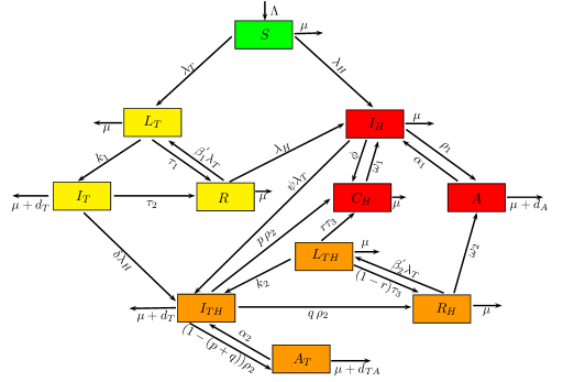
Figure 1. Model for TB-HIV/AIDS transmission.

2.1. Positivity and boundedness of solutions

Since the system of equations (3) represents human populations, all parameters in the model are non-negative and it can be shown that, given non-negative initial values, the solutions of the system are non-negative. Consider the biologically feasible region

$$\Omega=\{\left(S,L_{T},I_{T},R,I_{H},A,C_{H},L_{TH},I_{TH},R_{H},A_{T}\right)\in\mathbb{R}_{+}^{11}\,:\,N\leq\Lambda/\mu\}.$$

In what follows we prove the positive invariance of $\Omega$ (i.e., all solutions in $\Omega$ remain in $\Omega$ for all time). The rate of change of the total population, obtained by adding all the equations in model (3), is given by

$$\frac{dN}{dt}=\Lambda-\mu N(t)-d_{T}I_{T}(t)-d_{A}A(t)-d_{T}I_{TH}(t)-d_{TA}A_{T}(t).$$

Using a standard comparison theorem [25] we can show that

$$N(t)\leq N(0)e^{-\mu t}+\frac{\Lambda}{\mu}\left(1-e^{-\mu t}\right).$$

In particular, $N(t)\leq\frac{\Lambda}{\mu}$ if $N(0)\leq\frac{\Lambda}{\mu}$. Thus, the region $\Omega$ is positively invariant. Hence, it is sufficient to consider the dynamics of the flow generated by (3) in $\Omega$. In this region, the model is epidemiologically and mathematically well posed [20]. Thus, every solution of the model (3) with initial conditions in $\Omega$ remains in $\Omega$ for all $t>0$. This result is summarized below.

Lemma 2.1.

The region $\Omega$ is positively invariant for the model (3) with non-negative initial conditions in $\mathbb{R}^{11}_{+}$.

3. Analysis of the sub-models

In this section we analyze the models for HIV only (HIV-only model) and TB only (TB-only model).

3.1. HIV-only model

The model that considers only HIV (obtained by setting $L_{T}=I_{T}=R=L_{TH}=I_{TH}=R_{H}=A_{T}$) is given by

$$\begin{cases}\dot{S}(t)=\Lambda-\lambda_{H}(t)S(t)-\mu S(t),\\[5.69046pt] \dot{I}_{H}(t)=\lambda_{H}(t)S(t)-(\rho_{1}+\phi+\mu)I_{H}(t)+\alpha_{1}A(t)+\omega_{1}C_{H},\\[5.69046pt] \dot{A}(t)=\rho_{1}I_{H}(t)-(\alpha_{1}+\mu+d_{A})A(t),\\[5.69046pt] \dot{C}_{H}(t)=\phi I_{H}(t)-(\omega_{1}+\mu)C_{H}(t),\end{cases}$$ (4)

where

$$\lambda_{H}(t)=\frac{\beta_{2}}{N(t)}\left[I_{H}(t)+\eta_{C}C_{H}(t)+\eta_{A}A(t)\right]$$

with

$$N(t)=S(t)+I_{H}(t)+A(t)+C_{H}(t).$$

Analogously to Lemma 2.1, we can prove that the region

$$\Omega_{1}=\{\left(S,I_{H},A,C_{H}\right)\in\mathbb{R}_{+}^{4}\,:\,N\leq\Lambda/\mu\}$$ (5)

is positively invariant and attracting. Thus, the dynamics of the HIV-only model will be considered in $\Omega_{1}$.

3.1.1. Persistence

In this section, we look for the conditions under which the host population and disease will persist. Rewriting the submodel system (4) as

$$\begin{cases}\dot{S}(t)=\Lambda-\frac{\beta_{2}(N)\left(I_{H}+\eta_{C}\,C_{H}+\eta_{A}A\right)}{N}S(t)-\mu S(t),\\[5.69046pt] \dot{I}_{H}(t)=\frac{\beta_{2}(N)\left(I_{H}+\eta_{C}\,C_{H}+\eta_{A}A\right)}{N}S(t)-(\rho_{1}+\phi+\mu)I_{H}(t)+\alpha_{1}A(t)+\omega_{1}C_{H},\\[5.69046pt] \dot{C}_{H}(t)=\phi I_{H}(t)-(\omega_{1}+\mu)C_{H}(t),\\[5.69046pt] \dot{A}(t)=\rho_{1}I_{H}(t)-(\alpha_{1}+\mu+d_{A})A(t),\end{cases}$$ (6)

in what follows we assume that $\beta_{2}(N)$ is continuous for $N\geq 0$ and continuously differentiable for $N>0$; $\beta_{2}(N)$ is monotone nondecreasing in $N$; and $\beta_{2}(N)>0$ if $N>0$.

Remark 2.

In this work $\beta_{2}$ denotes the effective contact rate for HIV transmission. It is a constant for a concrete situation, but one can look to it as variable in the sense that, depending on the situation/region, one can have different values for this parameter. This is so because $\beta_{2}$ is related with the level of contagion/propagation of the disease. In Section 5 we consider fixed values for $\beta_{1}$ and $\beta_{2}$, which represent specific cases of the infection level. By varying $\beta_{1}$ and $\beta_{2}$ we vary the basic reproduction numbers (see expressions (12) and (20) for $R_{1}$ and $R_{2}$, respectively). Here we consider $\beta_{2}$ as a function of $N$ to discuss persistence.

It is convenient to reformulate the model in terms of the fractions of the $S$, $I_{H}$, $A$ and $C_{H}$ parts of the population,

$$x=\frac{S}{N},\quad y=\frac{I_{H}}{N},\quad z=\frac{C_{H}}{N},\quad w=\frac{A}{N},$$ (7)

and express (6) in these terms to obtain the system

$$\begin{cases}\dot{N}=\Lambda-(\mu+d_{A}w)N,\\[5.69046pt] \dot{x}=\frac{\Lambda}{N}(1-x)-\beta_{2}(N)(y+\eta_{C}z+\eta_{A}w)x+x(\mu-y+d_{A}w),\\[5.69046pt] \dot{y}=\beta_{2}(N)(y+\eta_{C}Z+\eta_{A}w)x+yd_{A}w-\left(\rho_{1}+\phi+\mu\right)y+\alpha_{1}w+\omega_{1}z,\\[5.69046pt] \dot{z}=\phi y-(\omega_{1}+\mu-d_{A}w)z,\\[5.69046pt] \dot{w}=\rho_{1}y-(\alpha_{1}+\mu+d_{A}-d_{A}w)w.\end{cases}$$ (8)

Equations (7) suggest that $x+y+z+w=1$. The manifold $x+y+z+w=1$, $x,y,z,w\geq 0$, is forward invariant under the solution flow of (8), which has a global solution satisfying (7). We now show conditions under which the host population will persist.

Theorem 3.1.

Let $\beta_{2}(0)=0$, $N(0)>0$. Then the population is uniformly persistent, that is,

$$\liminf_{t\to\infty}N(t)\geq\varepsilon,$$

where $\varepsilon>0$ does not depend on the initial data.

Proof.

We have to show that the set

$$X_{2}=\left\{N=0,\,x\geq 0,\,y\geq 0,\,z\geq 0,\,w\geq 0,\,x+y+z+w=1\right\}$$

is uniform strong repeller for

$$X_{1}=\left\{N>0,\,x\geq 0,\,y\geq 0,\,z\geq 0,\,w\geq 0,\,x+y+z+w=1\right\}.$$

Theorem 3.2, Theorem 3.3 and Corollary 1 are taken from [3, 44].

Theorem 3.2.

Let $X$ be a locally compact metric space with metric $d$. Let $X$ be the disjoint union of two sets $X_{1}$ and $X_{2}$ such that $X_{2}$ is compact. Let $\Phi$ be a continuous semiflow on $X_{1}$. Then $X_{2}$ is a uniform strong repeller for $X_{1}$, whenever it is a uniform weak repeller for $X_{1}$.

Theorem 3.3.

Let $D$ be a bounded interval in $\mathbb{R}$ and $g\,:\,(t_{0},\infty)\times D\to\mathbb{R}$ be bounded and uniformly continuous. Further, let $x\,:\,(t_{0},\infty)\to D$ be a solution of

$$x^{\prime}=g(t,x),$$

which is defined on the whole interval $(t_{0},\infty)$. Then there exist sequences $s_{n},t_{n}\to\infty$ such that

$$\lim_{n\to\infty}g(s_{n},x_{\infty})=0=\lim_{n\to\infty}g(t_{n},x^{\infty}).$$

Corollary 1.

Let the assumptions of Theorem 3.3 be satisfied. Then

• $\liminf_{t\to\infty}g(t,x_{\infty})\geq 0\geq\limsup_{t\to\infty}g(t,x_{\infty})$,

• $\liminf_{t\to\infty}g(t,x^{\infty})\geq 0\geq\limsup_{t\to\infty}g(t,x^{\infty})$.

As the assumptions of Theorem 3.2 are satisfied, it suffices to show that $X_{2}$ is a uniform weak repeller for $X_{1}$. Let $r=y+z+w$. Then,

$$\begin{split}r^{\prime}&=\beta_{2}(N)(yx+\eta_{C}zx+\eta_{A}wx)+d_{A}wr-\mu r-d_{A}w\\ &\leq\beta_{2}(N)(1+\eta_{C}+\eta_{A})-\frac{\Lambda}{N}r+d_{A}(r-1),\end{split}$$

using the fact that $x,y,z,w,r\leq 1$. This implies that

$$\begin{split}&\frac{\Lambda}{N^{\infty}}r^{\infty}+(1-r^{\infty})d_{A}\leq\beta_{2}(N^{\infty})(1+\eta_{C}+\eta_{A})\\ &\Rightarrow\beta_{2}(N^{\infty})\geq\frac{\Lambda r^{\infty}}{N^{\infty}\left(1+\eta_{C}+\eta_{A}\right)}+\frac{(1-r^{\infty})d_{A}}{1+\eta_{C}+\eta_{A}}.\end{split}$$ (9)

From the equation of $N$ in (8) we have

$$\liminf_{t\to\infty}\frac{1}{N}\frac{dN}{dt}\geq\frac{\Lambda}{N^{\infty}}-\left(\mu+d_{A}w^{\infty}\right)\geq\frac{\Lambda}{N^{\infty}}-\left(\mu+d_{A}r^{\infty}\right).$$

Hence $N$ increases exponentially, unless

$$\frac{\Lambda}{N^{\infty}}\leq\mu+d_{A}r^{\infty},\quad\text{that is,}\quad\frac{1}{d_{A}}\left(\frac{\Lambda}{N^{\infty}}-\mu\right)\leq r^{\infty}.$$ (10)

Combining (9) and (10), we obtain that

$$\beta_{2}(N^{\infty})\geq\left(\frac{\Lambda}{d_{A}N^{\infty}(1+\eta_{C}+\eta_{A})}-\frac{1}{1+\eta_{C}+\eta_{A}}\right)\left(\frac{\Lambda}{N^{\infty}}-\mu\right)+\frac{d_{A}}{1+\eta_{C}+\eta_{A}},$$ (11)

as $\beta_{2}(0)=0$ and $\beta_{2}(N)$ is continuous at $0$, $N^{\infty}\geq\varepsilon>0$ with $\varepsilon$ not depending on the initial data. From (11) we see that we can relax $\beta_{2}(0)=0$ and require

$$\beta_{2}(0)<\left(\frac{\Lambda}{d_{A}N^{\infty}(1+\eta_{C}+\eta_{A})}-\frac{1}{1+\eta_{C}+\eta_{A}}\right)\left(\frac{\Lambda}{N^{\infty}}-\mu\right)+\frac{d_{A}}{1+\eta_{C}+\eta_{A}}.$$

This concludes the proof. ∎

The disease is persistent in the population if the fraction of the infected and AIDS cases is bounded away from zero. If the population dies out and the fraction of the infected and AIDS remains bounded away from zero, we would still say that the disease is persistent in the population.

Proposition 3.4.

Let $\beta_{2}(\infty)(1+\eta_{C}+\eta_{A})\geq\frac{\Lambda}{N^{\infty}}r^{\infty}$. Then the disease is uniformly weakly persistent insofar as

$$r^{\infty}=\limsup_{t\to\infty}r(t)\geq\varepsilon,$$

with $\varepsilon>0$ being independent of the initial data, provided that $r(0)>0$.

The proof of Proposition 3.4 is outlined in [44].

3.1.2. Local stability of disease-free equilibrium

The model (4) has a disease-free equilibrium (DFE), obtained by setting the right-hand sides of the equations in the model to zero, given by

$$\Sigma_{0}=\left(S^{*},I^{*}_{H},A^{*},C^{*}_{H}\right)=\left(\frac{\Lambda}{\mu},0,0,0\right).$$

The linear stability of $\Sigma_{0}$ can be established using the next-generation operator method on the system (4). Following [46], the basic reproduction number is obtained as the spectral radius of the matrix $FV^{-1}$ at the DFE, $\Sigma_{0}$, with $F$ and $V$ given by, respectively,

$$F=\left[\begin{array}[]{cccc}0&0&0&0\\ \vskip 6.0pt plus 2.0pt minus 2.0pt\cr\lambda_{H}&{\frac{{\beta_{2}}\,S}{{N}}}&{\frac{{\beta_{2}}\,{\eta_{A}}\,S}{{N}}}&{\frac{{\beta_{2}}\,{\eta_{C}}\,S}{{N}}}\\ \vskip 6.0pt plus 2.0pt minus 2.0pt\cr 0&0&0&0\\ \vskip 6.0pt plus 2.0pt minus 2.0pt\cr 0&0&0&0\end{array}\right]$$

and

$$V=\left[\begin{array}[]{cccc}\lambda_{H}+\mu&{\frac{{\beta_{2}}\,S}{{N}}}&{\frac{{\beta_{2}}\,{\eta_{A}}\,S}{{N}}}&{\frac{{\beta_{2}}\,{\eta_{C}}\,S}{{N}}}\\ \vskip 6.0pt plus 2.0pt minus 2.0pt\cr 0&C_{1}&-{\alpha_{1}}&-{\omega_{1}}\\ \vskip 6.0pt plus 2.0pt minus 2.0pt\cr 0&-{\rho_{1}}&C_{2}&0\\ \vskip 6.0pt plus 2.0pt minus 2.0pt\cr 0&-\phi&0&C_{3}\end{array}\right],$$

where $C_{1}=\rho_{1}+\phi+\mu$, $C_{2}=\alpha_{1}+\mu+d_{A}$, $C_{3}=\omega_{1}+\mu$. The basic reproduction number is given by the dominant eigenvalue of the matrix $FV^{-1}$, that is,

$$R_{1}=\frac{{\beta_{2}}\,\Lambda\,\left(C_{3}(C_{2}+{\eta_{A}}\,{\rho_{1}})+{\eta_{C}}\,\phi C_{2}\right)}{N\mu\left[\mu\left(C_{3}(\rho_{1}+C_{2})+C_{2}\phi+\rho_{1}d_{A}\right)+\rho_{1}\omega_{1}d_{A}\right]}.$$ (12)

The basic reproduction number $R_{1}$ represents the expected average number of new HIV infections produced by a single HIV-infected individual when in contact with a completely susceptible population [46].

Remark 3.

The next-generation matrix is one of the most well known methods in epidemiology to compute the basic reproduction number for a compartmental model of the spread of infectious diseases. To calculate the basic reproduction number through this method, the whole population is divided into $n$ compartments in which there are $m<n$ infected compartments. Let $x_{i}$, $i=1,2,\ldots,m$, be the numbers of infected individuals in the $i$th infected compartment at time $t$. Now, the epidemic model is $x_{i}^{\prime}=F_{i}(x)-V_{i}(x)$ or, in vector form, $x^{\prime}=F(x)-V(x)$. Let $x_{0}$ denote here the disease-free equilibrium state. The Jacobian matrices of $F(x)$ and $V(x)$ are, respectively,

$$DF(x)=\left[\begin{array}[]{cc}F&0\\ 0&0\\ \end{array}\right]\quad\text{ and }\quad DV(x)=\left[\begin{array}[]{cc}V&0\\ J_{3}&J_{4}\\ \end{array}\right],$$

where $F$ and $V$ are the $m\times m$ matrices given by

$$F=\left[\frac{\partial F_{i}(x_{0})}{\partial x_{j}}\right],\quad V=\left[\frac{\partial V_{i}(x_{0})}{\partial x_{j}}\right].$$

The matrix $FV^{-1}$ is known as the next-generation matrix and its spectral radius is the basic reproduction number of the model. The reader interested in all the details about the computation of the basic reproduction number by the next-generation matrix is referred to [14, 46] or any good book on dynamical modeling and analysis of epidemics (e.g., [13]).

Lemma 3.5.

The disease free equilibrium $\Sigma_{0}$ is locally asymptotically stable if $R_{1}<1$, and unstable if $R_{1}>1$.

Proof.

Following Theorem 2 of [46], the disease-free equilibrium, $\Sigma_{0}$, is locally asymptotically stable if all the eigenvalues of the Jacobian matrix of the system (4), here denoted by $M\left(\Sigma_{0}\right)$, computed at the DFE $\Sigma_{0}$, have negative real parts. The Jacobian matrix of the system (4) at disease free equilibrium $\Sigma_{0}$ is given by

$$M\left(\Sigma_{0}\right)=\left[\begin{array}[]{cccc}-\mu&-{\frac{\beta_{2}\,\Lambda}{\mu\,N}}&-{\frac{\beta_{2}\,\eta_{A}\,\Lambda}{\mu\,N}}&-{\frac{\beta_{2}\,\eta_{C}\,\Lambda}{\mu\,N}}\\ \vskip 6.0pt plus 2.0pt minus 2.0pt\cr 0&{\frac{\beta_{2}\,\Lambda}{\mu\,N}}-C_{1}&{\frac{\beta_{2}\,\eta_{A}\,\Lambda}{\mu\,N}}+\alpha_{1}&{\frac{\beta_{2}\,\eta_{C}\,\Lambda}{\mu\,N}}+\omega_{1}\\ \vskip 6.0pt plus 2.0pt minus 2.0pt\cr 0&\rho_{1}&C_{2}&0\\ \vskip 6.0pt plus 2.0pt minus 2.0pt\cr 0&\phi&0&C_{3}\end{array}\right].$$ (13)

One has

$$\textrm{trace}\left[M\left(\Sigma_{0}\right)\right]=-\mu+{\frac{\beta_{2}\,\Lambda}{\mu\,N}}-(C_{1}+C_{2}+C_{3})<0$$

and

$$\det\left[M\left(\Sigma_{0}\right)\right]=-\frac{\beta_{2}\,\Lambda}{N}\left[C_{3}(C_{2}+\rho_{1}\eta_{A})+\phi\eta_{C}C_{2}\right]\\ +\mu\left[\mu\left(C_{3}(\rho_{1}+C_{2})+C_{2}\phi+\rho_{1}d_{A}\right)+\rho_{1}\omega_{1}d_{A}\right]>0$$

for $R_{1}<1$. We have just proved that the disease free equilibrium $\Sigma_{0}$ of model (4) is locally asymptotically stable if $R_{1}<1$, and unstable if $R_{1}>1$. ∎

3.1.3. Global stability of disease-free equilibrium (DFE)

Following [8], let us rewrite the submodel system (4) as

$$\begin{split}&\frac{dX}{dt}=F(X,Z),\\ &\frac{dZ}{dt}=G(X,Z),\quad G(X,0)=0,\end{split}$$ (14)

where $X=S$ and $Z=(I_{H},A,C_{H})$, with $X\in\mathbb{R}_{+}$ denoting the total number of uninfected individuals and $Z\in\mathbb{R}^{3}_{+}$ denoting the total number of infected individuals. The disease-free equilibrium is now denoted by

$$U_{0}=(X_{0},0),\quad\text{where}\,\,X_{0}=\left(\frac{\Lambda}{\mu},0\right).$$

The conditions (H1) and (H2) below must be met to guarantee global asymptotically stability:

• for $\frac{dX}{dt}=F(X,0)$, $U_{0}$ is globally asymptotically stable;

• $G(X,Z)=AZ-\hat{G}(X,Z)$, $\hat{G}(X,Z)\geq 0$ for $(X,Z)\in\mathcal{G}$, where $A=D_{Z}G(U_{0},0)$ is a Metzler matrix (the off diagonal elements of $A$ are nonnegative) and $\mathcal{G}$ is the region where the model makes biological sense.

Theorem 3.6.

The fixed point $U_{0}=(X_{0},0)$ is a globally asymptotically stable equilibrium of (4) provided $R_{1}<1$ and the assumptions (H1) and (H2) are satisfied.

Proof.

We have

$$\frac{dX}{dt}=F(X,Z)=\left[\begin{array}[]{c}\Lambda-\lambda_{H}S-\mu S\end{array}\right],$$

$$F(X,0)=\left[\begin{array}[]{c}\Lambda-\mu S\end{array}\right],$$

$$\frac{dZ}{dt}=G(X,Z)=\left[\begin{array}[]{c}\lambda_{H}(t)S(t)-C_{1}I_{H}(t)+\alpha_{1}A(t)+\omega_{1}C_{H}\\[5.69046pt] \rho_{1}I_{H}(t)-C_{2}A(t)\\[5.69046pt] \phi I_{H}(t)-C_{3}C_{H}(t)\end{array}\right],$$

and $G(X,0)=0$. Therefore,

$$\frac{dX}{dt}=F(X,0)=\left[\begin{array}[]{c}\Lambda-\mu S\\[5.69046pt] -\mu R_{T}\end{array}\right],$$

$$A=D_{Z}G(X_{0},0)=\left[\begin{array}[]{ccc}{\frac{\beta_{2}\,\Lambda}{N\mu}}-C_{1}&{\frac{\beta_{2}\,\eta_{A}\,\Lambda}{N\mu}}+\alpha_{1}&{\frac{\beta_{2}\,\eta_{C}\,\Lambda}{N\mu}}+\omega_{1}\\ \vskip 6.0pt plus 2.0pt minus 2.0pt\cr\rho_{1}&-C_{2}&0\\ \vskip 6.0pt plus 2.0pt minus 2.0pt\cr\phi&0&-C_{3}\end{array}\right]$$

and

$$\hat{G}(X,Z)=\left[\begin{array}[]{c}\hat{G}_{1}(X,Z)\\[5.69046pt] \hat{G}_{2}(X,Z)\\[5.69046pt] \hat{G}_{3}(X,Z)\end{array}\right]={\footnotesize{\left[\begin{array}[]{c}\beta_{2}(1-\frac{1}{N})(I_{H}+\eta_{A}A+\eta_{C}C_{H})\\ \vskip 6.0pt plus 2.0pt minus 2.0pt\cr 0\\ \vskip 6.0pt plus 2.0pt minus 2.0pt\cr 0\end{array}\right]}}.$$ (15)

It follows that $\hat{G}_{1}(X,Z)\geq 0$, $\hat{G}_{2}(X,Z)=\hat{G}_{3}(X,Z)=0$. Thus, $\hat{G}(X,Z)\geq 0$. Conditions (H1) and (H2) are satisfied, and we conclude that $U_{0}$ is globally asymptotically stable for $R_{1}<1$. ∎

3.1.4. Existence of an endemic equilibrium

To find conditions for the existence of an equilibrium for which HIV is endemic in the population (i.e., at least one of $I_{H}^{*}$, $A^{*}$ or $C_{H}^{*}$ is non-zero), denoted by $\Sigma_{H}=\left(S^{*},I_{H}^{*},A^{*},C_{H}^{*}\right)$, the equations in (4) are solved in terms of the force of infection at steady-state ($\lambda_{H}^{*}$), given by

$$\lambda_{H}^{*}=\frac{\beta_{2}\left(I_{H}^{*}+\eta_{A}A^{*}+\eta_{C}\,C_{H}^{*}\right)}{N^{*}}.$$ (16)

Setting the right hand sides of the model to zero (and noting that $\lambda_{H}=\lambda_{H}^{*}$ at equilibrium) gives

$$S^{*}=\frac{\Lambda}{\lambda_{H}^{*}+\mu},\quad I_{H}^{*}=-\frac{\lambda_{H}^{*}\Lambda C_{2}C_{3}}{D},\quad A^{*}=-\frac{\rho_{1}\lambda_{H}^{*}\Lambda C_{3}}{D},\quad C_{H}^{*}=-\frac{\phi\lambda_{H}^{*}\Lambda C_{2}}{D},$$ (17)

with $D=-(\lambda_{H}^{*}+\mu)(\mu\left(C_{3}(\rho_{1}+C_{2})+C_{2}\phi+\rho_{1}d_{A}\right)+\rho_{1}\omega_{1}d_{A})$. Using (17) in the expression for $\lambda_{H}^{*}$ in (16) shows that the nonzero (endemic) equilibria of the model satisfy

$$\lambda_{H}^{*}=\frac{\Lambda\beta_{2}\left(C_{2}C_{3}+\eta_{A}\rho_{1}C_{3}+\eta_{C}\phi C_{2}\right)}{N\left[\mu\left(C_{3}(\rho_{1}+C_{2})+C_{2}\phi+\rho_{1}d_{A}\right)+\rho_{1}\omega_{1}d_{A}\right]}-\mu,$$

that is,

$$\lambda_{H}^{*}=-\mu(1-R_{1}).$$

The force of infection at the steady-state $\lambda_{H}^{*}$ is positive, only if $R_{1}>1$. We have just proved the following result.

Lemma 3.7.

The submodel system (4) has a unique endemic equilibrium whenever $R_{1}>1$.

3.1.5. Local stability of the endemic equilibrium

In what follows we prove the local asymptotic stability of the endemic equilibrium $\Sigma_{H}$, using the center manifold theory [6], as described in [9, Theorem 4.1], with $\Sigma_{H}=(S^{*},I_{H}^{*},A^{*},C_{H}^{*})$ and each of its components given as in (17). To apply this method, the following simplification and change of variables are first made. Let $S=x_{1}$, $I_{H}=x_{2}$, $A=x_{3}$ and $C_{H}=x_{4}$, so that $N=x_{1}+x_{2}+x_{3}+x_{4}$. Further, by using vector notation $X=(x_{1},x_{2},x_{3},x_{4})^{T}$, the submodel (4) can be written in the form $\frac{dX}{dt}=(f_{1},f_{2},f_{3},f_{4})^{T}$, as follows:

$$\begin{split}\frac{dx_{1}}{dt}&=f_{1}=\Lambda-\frac{\beta_{2}\left(x_{2}+\eta_{A}x_{3}+\eta_{C}x_{4}\right)}{x_{1}+x_{2}+x_{3}+x_{4}}x_{1}-\mu x_{1},\\[5.69046pt] \frac{dx_{2}}{dt}&=f_{2}=\frac{\beta_{2}\left(x_{2}+\eta_{A}x_{3}+\eta_{C}x_{4}\right)}{x_{1}+x_{2}+x_{3}+x_{4}}x_{1}-C_{1}x_{2}+\alpha_{1}x_{3}+\omega_{1}x_{4},\\[5.69046pt] \frac{dx_{3}}{dt}&=f_{3}=\rho_{1}x_{2}-C_{2}x_{3},\\[5.69046pt] \frac{dx_{4}}{dt}&=f_{4}=\phi x_{2}-C_{3}x_{4}.\end{split}$$ (18)

The basic reproduction number of the submodel (4) is given by (12). Choose as bifurcation parameter $\beta^{*}$, by solving for $\beta_{2}$ from $R_{1}=1$:

$$\beta^{*}=\frac{\mu\left(C_{3}(\rho_{1}+C_{2})+C_{2}\phi+\rho_{1}d_{A}\right)+\rho_{1}\omega_{1}d_{A}}{C_{3}(C_{2}+{\eta_{A}}\,{\rho_{1}})+{\eta_{C}}\,\phi C_{2}}.$$

The submodel (4) has a disease free equilibrium given by

$$\Sigma_{H}=(x_{10},x_{20},x_{30},x_{40})=\left(\frac{\Lambda}{\mu},0,0,0\right).$$

The Jacobian of the system (18), evaluated at $\Sigma_{0}$, $M\left(\Sigma_{0}\right)$, and with $\beta_{2}=\beta^{*}$, is given by (13). Note that the above linearized system, of the transformed system (18) with $\beta_{2}=\beta^{*}$, has a zero eigenvalue which is simple. Hence, the center manifold theory [6] can be used to analyze the dynamics of (18) near $\beta_{2}=\beta^{*}$. In particular, Theorem 4.1 in [9] is used to show the locally asymptotically stability of the endemic equilibrium point of (18), for $\beta_{2}$ near $\beta^{*}$.

The Jacobian $M(\Sigma_{0})$ at $\beta_{2}=\beta^{*}$ has a right eigenvector (associated with the zero eigenvalue) given by $w=[w_{1},w_{2},w_{3},w_{4}]^{T}$, where

$$\begin{split}w_{1}&=-{\frac{w_{3}\,\mu(C_{3}(\rho_{1}+C_{2})+C_{2}\phi+\rho_{1}d_{A})+\rho_{1}\omega_{1}d_{A}}{C_{3}\mu\,\rho_{1}}},\\ w_{2}&={\frac{w_{3}\,C_{2}}{\rho_{1}}},\\ w_{3}&=w_{3}>0,\\ w_{4}&={\frac{C_{2}\phi\,w_{3}}{C_{3}\rho_{1}}}.\end{split}$$

Further, $M(\Sigma_{0})$ for $\beta_{2}=\beta^{*}$ has a left eigenvector $v=[v_{1},v_{2},v_{3},v_{4}]$ (associated with the zero eigenvalue), where

$$\begin{split}v_{1}&=0,\\ v_{2}&=v_{3}{\frac{C_{2}C_{3}+\eta_{A}\rho_{1}C_{3}+\eta_{C}\phi C_{2}}{\mu(\eta_{A}C_{1}+\eta_{A}\omega_{1}+\alpha_{1})+\omega_{1}\eta_{A}\rho_{1}+(\eta_{C}\phi+\omega_{1})\alpha_{1}}},\\ v_{3}&=v_{3}>0,\\ v_{4}&=v_{3}{\frac{\eta_{C}C_{2}+\mu(\omega_{1}+\eta_{C}\rho_{1}+\eta_{C}\phi)+\rho_{1}(\omega_{1}\eta_{A}+\eta_{C}d_{A})+(\omega_{1}+\eta_{C}\phi)(\alpha_{1}+d_{A})}{\mu\left(\eta_{A}C_{1}+\eta_{A}\omega_{1}+\alpha_{1}\right)+\omega_{1}(\eta_{A}\rho_{1}+\alpha_{1})+\eta_{C}\phi\alpha_{1}}}.\end{split}$$

To apply Theorem 4.1 in [9] it is convenient to let $f_{k}$ represent the right-hand side of the $k$th equation of the system (18) and let $x_{k}$ be the state variable whose derivative is given by the $k$th equation for $k=1,\ldots,4$. The local stability near the bifurcation point $\beta_{2}=\beta^{*}$ is then determined by the signs of two associated constants, denoted by $a$ and $b$, defined (respectively) by

$$a=\sum_{k,i,j=1}^{4}\,v_{k}w_{i}w_{j}\frac{\partial^{2}f_{k}}{\partial x_{i}\partial x_{j}}(0,0)\quad\text{and}\quad b=\sum_{k,i=1}^{4}\,v_{k}w_{i}\frac{\partial^{2}f_{k}}{\partial x_{i}\partial\phi}(0,0)$$

with $\phi=\beta_{2}-\beta^{*}$. Note that, in $f_{k}(0,0)$, the first zero corresponds to the DFE, $\Sigma_{0}$, for the subsystem (4). In other words, $f_{k}(0,\phi)=0$, for $k=1,\ldots,4$, if and only if the right-hand sides of the equations of (4) is zero at $\Sigma_{0}$. Moreover, from $\phi=\beta_{2}-\beta^{*}$ we have $\phi=0$ when $\beta_{2}=\beta^{*}$, which is the second component in $f_{k}(0,0)$.

For the system (18), the associated non-zero partial derivatives at the disease free equilibrium $\Sigma_{0}$ are given by

$$\begin{split}&\frac{\partial^{2}f_{1}}{\partial x_{2}^{2}}=\frac{2\beta^{*}\mu}{\Lambda},\quad\frac{\partial^{2}f_{1}}{\partial x_{2}\partial x_{3}}=\frac{\beta^{*}\mu(1+\eta_{A})}{\Lambda},\quad\frac{\partial^{2}f_{1}}{\partial x_{2}\partial x_{4}}=\frac{\beta^{*}\mu(1+\eta_{C})}{\Lambda},\\ &\frac{\partial^{2}f_{1}}{\partial x_{3}^{2}}=\frac{2\beta^{*}\mu\eta_{A}}{\Lambda},\quad\frac{\partial^{2}f_{1}}{\partial x_{3}\partial x_{4}}=\frac{\beta^{*}\mu(\eta_{A}+\eta_{C})}{\Lambda},\\ &\frac{\partial^{2}f_{1}}{\partial x_{4}\partial x_{2}}=\frac{\beta^{*}\mu(1+\eta_{C})}{\Lambda},\quad\frac{\partial^{2}f_{1}}{\partial x_{4}^{2}}=\frac{2\beta^{*}\mu\eta_{C}}{\Lambda},\\ &\frac{\partial^{2}f_{2}}{\partial x_{2}^{2}}=\frac{2\beta^{*}\mu}{\Lambda},\quad\frac{\partial^{2}f_{2}}{\partial x_{2}\partial x_{3}}=-\frac{\beta^{*}\mu(1+\eta_{A})}{\Lambda},\quad\frac{\partial^{2}f_{2}}{\partial x_{2}\partial x_{4}}=-\frac{\beta^{*}\mu(1+\eta_{C})}{\Lambda},\\ &\frac{\partial^{2}f_{2}}{\partial x_{3}^{2}}=-\frac{2\beta^{*}\eta_{A}\mu}{\Lambda},\quad\frac{\partial^{2}f_{2}}{\partial x_{3}\partial x_{4}}=-\frac{\beta^{*}\mu(\eta_{A}+\eta_{C})}{\Lambda},\\ &\frac{\partial^{2}f_{2}}{\partial x_{4}^{2}}=-\frac{2\beta^{*}\eta_{C}\mu}{\Lambda},\quad\frac{\partial^{2}f_{2}}{\partial x_{4}\partial x_{2}}=-\frac{\beta^{*}\mu(1+\eta_{C})}{\Lambda}.\end{split}$$

It follows from the above expressions that

$$a=\frac{w_{3}^{2}C_{2}\phi\,\beta_{2}\mu\left(\eta_{A}+\eta_{C}\right)}{\rho_{1}\left(\omega_{1}+\mu\right)\Lambda}-\frac{2D_{1}C_{2}^{2}\left(C_{3}+\phi(1+\eta_{C})\right)}{D_{2}\rho_{1}^{2}C_{3}}\\ -\frac{2D_{1}\left(C_{2}C_{3}\rho_{1}\left(C_{3}(1+\eta_{A})+\phi\right)+C_{3}^{2}\eta_{A}\rho_{1}^{2}+C_{2}^{2}\phi^{2}\eta_{C}\right)}{D_{2}\rho_{1}^{2}C_{3}^{2}},$$

with

$$\begin{split}D_{1}&=v_{3}w_{3}^{2}\beta_{2}\mu\left(C_{3}C_{2}+C_{3}\eta_{A}\rho_{1}+\eta_{C}\phi C_{2}\right),\\ D_{2}&=\Lambda\left(\eta_{A}\rho_{1}C_{3}+C_{3}\alpha_{1}+\eta_{A}\mu C_{3}+\mu\phi+\eta_{C}\phi\alpha_{1}\right).\end{split}$$

For the sign of $b$, it can be shown that the associated non-vanishing partial derivatives are

$$\begin{split}\frac{\partial^{2}f_{1}}{\partial x_{2}\partial\beta^{*}}&=-1,\quad\frac{\partial^{2}f_{1}}{\partial x_{3}\partial\beta^{*}}=-\eta_{A},\quad\frac{\partial^{2}f_{1}}{\partial x_{4}\partial\beta^{*}}=-\eta_{C},\\ \frac{\partial^{2}f_{2}}{\partial x_{2}\partial\beta^{*}}&=-1,\quad\frac{\partial^{2}f_{2}}{\partial x_{3}\partial\beta^{*}}=-\eta_{A},\quad\frac{\partial^{2}f_{2}}{\partial x_{4}\partial\beta^{*}}=\eta_{C}.\end{split}$$

It also follows from the above expressions that

$$b={\frac{((\eta_{A}+\eta_{C})\rho_{1}+C_{2})\left(C_{3}C_{2}+C_{3}\eta_{A}\rho_{1}+\eta_{C}\phi C_{2}\right)v_{3}w_{3}}{\left((\eta_{A}\rho_{1}+\alpha_{1}+\eta_{A}\mu)C_{3}+\eta_{A}\mu\phi+\eta_{C}\phi\alpha_{1}\right)\rho_{1}}}.$$

From the previous computations, we have $a<0$ and $b>0$. Thus, using Theorem 4.1 of [9], the following result is established.

Theorem 3.8.

The endemic equilibrium $\Sigma_{H}$ is locally asymptotically stable for the basic reproduction number $R_{1}$ (12) near 1.

3.2. TB-only model

The sub-model of (3) with no HIV/AIDS disease, that is, $I_{H}=A=C_{H}=L_{TH}=I_{TH}=R_{H}=A_{T}=0$, is given by

$$\begin{cases}\dot{S}(t)=\Lambda-\lambda_{T}(t)S(t)-\mu S(t),\\[5.69046pt] \dot{L}_{T}(t)=\lambda_{T}(t)S(t)+\beta^{{}^{\prime}}_{1}\lambda_{T}(t)R(t)-(k_{1}+\tau_{1}+\mu)L_{T}(t),\\[5.69046pt] \dot{I}_{T}(t)=k_{1}L_{T}(t)-(\tau_{2}+d_{T}+\mu)I_{T}(t),\\[5.69046pt] \dot{R}(t)=\tau_{1}L_{T}(t)+\tau_{2}I_{T}(t)-(\beta^{{}^{\prime}}_{1}\lambda_{T}(t)+\mu)R(t),\end{cases}$$ (19)

where

$$\lambda_{T}(t)=\frac{\beta_{1}I_{T}(t)}{N(t)}$$

and

$$N(t)=S(t)+L_{T}(t)+I_{T}(t)+R(t).$$

The sub-model (19) was proposed and analyzed in [7]. This model incorporates the basic properties of TB transmission and dynamics. The basic reproduction number $R_{2}$ of (19) is given by

$$R_{2}=\frac{\Lambda}{\mu N}\left(\frac{\beta_{1}}{\mu+d_{T}+\tau_{2}}\right)\left(\frac{k_{1}}{\mu+k_{1}+\tau_{1}}\right).$$ (20)

The existence, uniqueness and local asymptotic stability of the disease-free and endemic equilibria are proven in [7, Theorem 1].

4. Analysis of the full model

We now consider the full model (3), with the DFE given by

$$\begin{split}\Xi_{0}&=\left(S^{\diamond},L_{T}^{\diamond},I_{T}^{\diamond},R^{\diamond},I_{H}^{\diamond},A^{\diamond},C_{H}^{\diamond},L_{TH}^{\diamond},I_{TH}^{\diamond},R_{H}^{\diamond},A_{T}^{\diamond}\right)\\ &=\left(\frac{\Lambda}{\mu},0,0,0,0,0,0,0,0,0,0\right).\end{split}$$

The associated matrices $F$ and $V$ (see Section 3.1.2) are given, respectively, by

$$F=\left[\begin{array}[]{cc}F_{1}&F_{2}\end{array}\right]$$

with

$$F_{1}=\left[\begin{array}[]{cccccc}0&0&0&0&0&0\\ \vskip 6.0pt plus 2.0pt minus 2.0pt\cr\lambda_{T}&0&{\frac{\beta_{1}(S+R\beta^{\prime}_{1})}{N}}&\beta^{\prime}_{1}\lambda_{T}&0&0\\ \vskip 6.0pt plus 2.0pt minus 2.0pt\cr 0&0&0&0&0&0\\ \vskip 6.0pt plus 2.0pt minus 2.0pt\cr 0&0&0&0&0&0\\ \vskip 6.0pt plus 2.0pt minus 2.0pt\cr\lambda_{H}&0&0&\lambda_{H}&{\frac{\beta_{2}(S+R)}{N}}&{\frac{\beta_{2}\eta_{A}(S+R)}{N}}\\ \vskip 6.0pt plus 2.0pt minus 2.0pt\cr 0&0&0&0&0&0\\ \vskip 6.0pt plus 2.0pt minus 2.0pt\cr 0&0&0&0&0&0\\ \vskip 6.0pt plus 2.0pt minus 2.0pt\cr 0&0&{\frac{\beta^{\prime}_{2}\,\beta_{1}R_{H}}{N}}&0&0&0\\ \vskip 6.0pt plus 2.0pt minus 2.0pt\cr 0&0&\delta\lambda_{H}+{\frac{\psi\,\beta_{1}I_{H}}{N}}&0&{\frac{\delta\beta_{2}I_{T}}{N}}+\psi\lambda_{T}&{\frac{\delta\beta_{2}\eta_{A}I_{T}}{N}}\\ \vskip 6.0pt plus 2.0pt minus 2.0pt\cr 0&0&0&0&0&0\\ \vskip 6.0pt plus 2.0pt minus 2.0pt\cr 0&0&0&0&0&0\end{array}\right],$$

$$F_{2}=\left[\begin{array}[]{ccccc}0&0&0&0&0\\ \vskip 6.0pt plus 2.0pt minus 2.0pt\cr 0&0&{\frac{\beta_{1}(S+R\beta^{\prime}_{1})}{N}}&0&{\frac{\beta_{1}(S+R\beta^{\prime}_{1})}{N}}\\ \vskip 6.0pt plus 2.0pt minus 2.0pt\cr 0&0&0&0&0\\ \vskip 6.0pt plus 2.0pt minus 2.0pt\cr 0&0&0&0&0\\ \vskip 6.0pt plus 2.0pt minus 2.0pt\cr{\frac{\beta_{2}\eta_{C}(S+R)}{N}}&{\frac{\beta_{2}(S+R)}{N}}&{\frac{\beta_{2}(S+R)}{N}}&{\frac{\beta_{2}(S+R)}{N}}&{\frac{\beta_{2}\eta_{A}(S+R)}{N}}\\ \vskip 6.0pt plus 2.0pt minus 2.0pt\cr 0&0&0&0&0\\ \vskip 6.0pt plus 2.0pt minus 2.0pt\cr 0&0&0&0&0\\ \vskip 6.0pt plus 2.0pt minus 2.0pt\cr 0&{\frac{\beta^{\prime}_{2}\,\beta_{1}R_{H}}{N}}&\beta^{\prime}_{2}\lambda_{T}&{\frac{\beta^{\prime}_{2}\,\beta_{1}R_{H}}{N}}&0\\ \vskip 6.0pt plus 2.0pt minus 2.0pt\cr{\frac{\delta\beta_{2}I_{T}}{N}}&{\frac{\delta\beta_{2}I_{T}}{N}}+{\frac{\psi\beta_{1}I_{H}}{N}}&\frac{\delta\beta_{2}I_{T}}{N}&{\frac{\delta\beta_{2}\eta_{A}I_{T}}{N}}+{\frac{\psi\beta_{1}I_{H}}{N}}&0\\ \vskip 6.0pt plus 2.0pt minus 2.0pt\cr 0&0&0&0&0\\ \vskip 6.0pt plus 2.0pt minus 2.0pt\cr 0&0&0&0&0\end{array}\right],$$

and $V=\left[V_{1}\quad V_{2}\right]$ with

$$V_{1}=\left[\begin{array}[]{cccccc}\lambda_{T}+\lambda_{H}+\mu&0&{\frac{\beta_{1}S}{N}}&0&{\frac{\beta_{2}S}{N}}&{\frac{\beta_{2}S\eta_{A}}{N}}\\ \vskip 6.0pt plus 2.0pt minus 2.0pt\cr 0&C_{4}&0&0&0&0\\ \vskip 6.0pt plus 2.0pt minus 2.0pt\cr 0&-k_{1}&\delta\lambda_{H}+C_{5}&0&{\frac{\delta\beta_{2}I_{T}}{N}}&{\frac{\delta\beta_{2}\eta_{A}I_{T}}{N}}\\ \vskip 6.0pt plus 2.0pt minus 2.0pt\cr 0&-\tau_{1}&\frac{\beta^{\prime}_{1}\beta_{1}R-\tau_{2}N}{N}&\beta^{\prime}_{1}\lambda_{T}+\lambda_{H}+\mu&{\frac{\beta_{2}R}{N}}&{\frac{\beta_{2}\eta_{A}R}{N}}\\ \vskip 6.0pt plus 2.0pt minus 2.0pt\cr 0&0&{\frac{\psi\beta_{1}I_{H}}{N}}&0&\psi\lambda_{T}+C_{1}&-\alpha_{1}\\ \vskip 6.0pt plus 2.0pt minus 2.0pt\cr 0&0&0&0&-\rho_{1}&C_{2}\\ \vskip 6.0pt plus 2.0pt minus 2.0pt\cr 0&0&0&0&-\phi&0\\ \vskip 6.0pt plus 2.0pt minus 2.0pt\cr 0&0&0&0&0&0\\ \vskip 6.0pt plus 2.0pt minus 2.0pt\cr 0&0&0&0&0&0\\ \vskip 6.0pt plus 2.0pt minus 2.0pt\cr 0&0&{\frac{\beta^{\prime}_{2}\beta_{1}R_{H}}{N}}&0&0&0\\ \vskip 6.0pt plus 2.0pt minus 2.0pt\cr 0&0&0&0&0&0\end{array}\right]$$

and

$$V_{2}=\left[\begin{array}[]{ccccc}{\frac{\beta_{2}\eta_{C}S}{N}}&{\frac{\beta_{2}S}{N}}&{\frac{\left(\beta_{1}+\beta_{2}\right)S}{N}}&{\frac{\beta_{2}S}{N}}&{\frac{\left(\beta_{1}+\beta_{2}\eta_{A}\right)S}{N}}\\ \vskip 6.0pt plus 2.0pt minus 2.0pt\cr 0&0&0&0&0\\ \vskip 6.0pt plus 2.0pt minus 2.0pt\cr{\frac{\delta\beta_{2}\eta_{C}I_{T}}{N}}&{\frac{\delta\beta_{2}I_{T}}{N}}&{\frac{\delta\beta_{2}I_{T}}{N}}&{\frac{\delta\beta_{2}I_{T}}{N}}&{\frac{\delta\beta_{2}\eta_{A}I_{T}}{N}}\\ \vskip 6.0pt plus 2.0pt minus 2.0pt\cr\frac{\beta_{2}\eta_{C}R}{N}&{\frac{\beta_{2}R}{N}}&{\frac{\left(\beta^{\prime}_{1}\beta_{1}+\beta_{2}\right)R}{N}}&{\frac{\beta_{2}R}{N}}&\frac{\left(\beta^{\prime}_{1}\beta_{1}+\beta_{2}\eta_{A}\right)R}{N}\\ \vskip 6.0pt plus 2.0pt minus 2.0pt\cr-\omega_{1}&0&{\frac{\psi\beta_{1}I_{H}}{N}}&0&\frac{\psi\beta_{1}I_{H}}{N}\\ \vskip 6.0pt plus 2.0pt minus 2.0pt\cr 0&{\frac{\beta_{2}R}{N}}&0&-\omega_{2}&0\\ \vskip 6.0pt plus 2.0pt minus 2.0pt\cr\omega_{1}+\mu&-r\,\tau_{3}&-p\,\rho_{2}&0&0\\ \vskip 6.0pt plus 2.0pt minus 2.0pt\cr 0&C_{6}&0&0&0\\ \vskip 6.0pt plus 2.0pt minus 2.0pt\cr 0&-k_{2}&C_{7}&0&-\alpha_{2}\\ \vskip 6.0pt plus 2.0pt minus 2.0pt\cr 0&\left(-1+r\right)\tau_{3}&-q\,\rho_{2}+{\frac{\beta^{\prime}_{2}\beta_{1}R_{H}}{N}}&\beta^{\prime}_{2}\lambda_{T}+\omega_{2}+\mu&{\frac{\beta^{\prime}_{2}\beta_{1}R_{H}}{N}}\\ \vskip 6.0pt plus 2.0pt minus 2.0pt\cr 0&0&\left(-1+p+q\right)\rho_{2}&0&C_{8}\end{array}\right],$$

where $C_{4}=k_{1}+\tau_{1}+\mu$, $C_{5}=\tau_{2}+\mu+d_{T}$, $C_{6}=k_{2}+\tau_{3}+\mu$, $C_{7}=\rho_{2}+\mu+d_{T}$ and $C_{8}=\alpha_{2}+d_{TA}+\mu$. The dominant eigenvalues of the matrix $FV^{-1}$ are

$$R_{1}=\frac{{\beta_{2}}\,\Lambda\,\left(C_{3}(C_{2}+{\eta_{A}}\,{\rho_{1}})+{\eta_{C}}\,\phi C_{2}\right)}{N\mu\left[\mu\left(C_{3}(\rho_{1}+C_{2})+C_{2}\phi+\rho_{1}d_{A}\right)+\rho_{1}\omega_{1}d_{A}\right]},\quad R_{2}=\frac{\Lambda\beta_{1}k_{1}}{\mu NC_{5}C_{4}}.$$

Thus, the basic reproduction number $R_{0}$ of the model (21) is given by

$$R_{0}=\max\{R_{1},R_{2}\}.$$

Using the same procedure as in Section 3.1.2, the following result holds.

Lemma 4.1.

The DFE of the full HIV-TB model (3), given by $\Xi_{0}$, is locally asymptotically stable if $R_{0}<1$, and unstable if $R_{0}>1$.

Remark 4.

There are different ways to compute the basic reproduction number $R_{0}$. Here we are computing it using one of the most well-known methods: $R_{0}$ is the dominant eigenvalue of the associated next-generation matrix $FV^{-1}$ (see Remark 3). A justification for the value of the basic reproduction number $R_{0}$ to be $\max\{R_{1},R_{2}\}$ is given in Section 4.4 of [46].

5. Optimal control problem

In this section we present an optimal control problem, describing our goal and the restrictions of the epidemic. In the model without controls discussed so far, we have $p$ representing the fraction of $I_{TH}$ individuals that take HIV and TB treatment and $q$ representing the fraction of $I_{TH}$ individuals that take TB treatment only. Roughly speaking, the problem of optimal control consists to determine the optimal combination for the values of $p$ and $q$. For this reason, we take $p$ as the control $u_{1}$ and $q$ as the control $u_{2}$. Precisely, we add to the model (3) the two control functions $u_{1}(\cdot)$ and $u_{2}(\cdot)$ in the following way:

$$\begin{cases}\dot{S}(t)=\Lambda-\lambda_{T}(t)S(t)-\lambda_{H}(t)S(t)-\mu S(t),\\[5.69046pt] \dot{L}_{T}(t)=\lambda_{T}(t)S(t)+\beta^{{}^{\prime}}_{1}\lambda_{T}(t)R(t)-\left(k_{1}+\tau_{1}+\mu\right)L_{T}(t),\\[5.69046pt] \dot{I}_{T}(t)=k_{1}L_{T}(t)-\left(\tau_{2}+d_{T}+\mu+\delta\lambda_{H}(t)\right)I_{T}(t),\\[5.69046pt] \dot{R}(t)=\tau_{1}L_{T}(t)+\tau_{2}I_{T}(t)-(\beta^{{}^{\prime}}_{1}\lambda_{T}(t)+\lambda_{H}(t)+\mu)R(t),\\[5.69046pt] \dot{I}_{H}(t)=\lambda_{H}(t)S(t)-(\rho_{1}+\phi+\psi\lambda_{T}(t)+\mu)I_{H}(t)+\alpha_{1}A(t)+\lambda_{H}(t)R(t)+\omega_{1}C_{H}(t),\\[5.69046pt] \dot{A}(t)=\rho_{1}I_{H}(t)+\omega_{2}R_{H}(t)-\alpha_{1}A(t)-(\mu+d_{A})A(t),\\[5.69046pt] \dot{C}_{H}(t)=\phi I_{H}(t)+u_{1}(t)\,\rho_{2}I_{TH}(t)+r\,\tau_{3}L_{TH}(t)-(\omega_{1}+\mu)C_{H}(t),\\[5.69046pt] \dot{L}_{TH}(t)=\beta^{{}^{\prime}}_{2}\lambda_{T}(t)R_{H}(t)-\left(k_{2}+\tau_{3}+\mu\right)L_{TH}(t),\\[5.69046pt] \dot{I}_{TH}(t)=\delta\lambda_{H}(t)I_{T}(t)+\psi\lambda_{T}(t)I_{H}(t)+\alpha_{2}A_{T}(t)+k_{2}L_{TH}(t)-\left(\rho_{2}+\mu+d_{T}\right)I_{TH}(t),\\[5.69046pt] \dot{R}_{H}(t)=u_{2}(t)\rho_{2}I_{TH}(t)+(1-r)\,\tau_{3}L_{TH}(t)-\left(\beta^{{}^{\prime}}_{2}\lambda_{T}(t)+\omega_{2}+\mu\right)R_{H}(t),\\[5.69046pt] \dot{A}_{T}(t)=\left(1-(u_{1}(t)+u_{2}(t))\right)\rho_{2}I_{TH}(t)-\left(\alpha_{2}+\mu+d_{TA}\right)A_{T}(t).\end{cases}$$ (21)

As already mentioned, the controls $u_{1}$ and $u_{2}$ represent the fraction of $I_{TH}$ individuals that are treated for TB and HIV (simultaneously) and treated for TB only, respectively. If we consider fixed values for $u_{1}$ and $u_{2}$ in (21), then we get the model (3) with $u_{1}=p$ and $u_{2}=q$. The aim is to find the optimal values $u_{1}^{*}$ and $u_{2}^{*}$ of the controls $u_{1}$ and $u_{2}$, such that the associated state trajectories $S^{*},L_{T}^{*},I_{T}^{*},R^{*},I_{H}^{*},A^{*},C_{H}^{*},L_{TH}^{*},I_{TH}^{*},R_{H}^{*},A_{T}^{*}$, solution of the system (21) in the time interval $[0,T]$ with initial conditions $S^{*}(0)$, $L_{T}^{*}(0)$, $I_{T}^{*}(0)$, $R^{*}(0)$, $I_{H}^{*}(0)$, $A^{*}(0)$, $C_{H}^{*}(0)$, $L_{TH}^{*}(0)$, $I_{TH}^{*}(0)$, $R_{H}^{*}(0)$, $A_{T}^{*}(0)$, minimize the objective functional. Here the objective functional considers the number of HIV-infected individuals with AIDS symptoms co-infected with TB $A_{T}$, and the implementation cost of the strategies associated to the controls $u_{i}$, $i=1,2$. The controls are bounded between $0$ and $0.95$. We assume that $p$ and $q$ cannot take values greater than $0.95$ because we assume that there are some budgetary constraints or some resistance from patients in making the treatments (treatment for HIV and TB together or just the treatment for TB). In other words, we assume that one cannot treat all the people for both diseases or even just for tuberculosis. This is more than reasonable from biological side. Moreover, the sum of $p+q$ is also taken as bounded by 0.95. This is related with the formulation of the model. Indeed, note that $1-(p+q)$ is the fraction of $I_{TH}$ individuals who are not treated for TB and HIV simultaneously and are also not treated for TB alone. For this reason, what we assume is that this fraction of individuals takes at least the value of 5%. This is in agreement with available medical data. Precisely, we consider the state system (21) of ordinary differential equations in $\mathbb{R}^{11}$ with the set of admissible control functions given by

$$\Theta=\biggl{\{}(u_{1}(\cdot),u_{2}(\cdot))\in(L^{\infty}(0,T))^{2}\,|\,0\leq u_{1}(t),u_{2}(t)\leq 0.95\,\\ \text{ and }\,0\leq u_{1}(t)+u_{2}(t)\leq 0.95,\,\forall\,t\in[0,T]\,\biggr{\}}.$$ (22)

The objective functional is given by

$$J(u_{1}(\cdot),u_{2}(\cdot))=\int_{0}^{T}\left[A_{T}(t)+\frac{W_{1}}{2}u_{1}^{2}(t)+\frac{W_{2}}{2}u_{2}^{2}(t)\right]dt,$$ (23)

where the constants $W_{1}$ and $W_{2}$ are a measure of the relative cost of the interventions associated to the controls $u_{1}$ and $u_{2}$, respectively.

Remark 5.

Epidemiologically, our cost functional tells us that we want to minimize the number of HIV-infected individuals with AIDS symptoms co-infected with active TB. For that, one applies control measures that are associated with some implementation costs that we also intend to minimize. Other cost functionals may be used as well. Here, by considering the cost with controls in a quadratic form, we are being consistent with previous works in the literature (see, e.g., [35, 42]). Moreover, a quadratic structure in the control has mathematical advantages: if the control set is a compact and convex polyhedron (as it is the case here), it imply that the Hamiltonian attains its minimum over the control set at a unique point. For future work we plan to compare the results now obtained, for a cost with a quadratic form in the controls, with those of a linear cost in the controls.

In order to simplify the formulation of the optimal control problem, let $f_{i}$ represent the right-hand side of the $i$th equation of system (21), $x_{i}$ be the state variable whose derivative is given by the $i$th component of $F$, $F=\left(f_{1},\ldots,f_{11}\right)$, and $X=\left(x_{1},\ldots,x_{11}\right)$, $i=1,\ldots,11$. We consider the optimal control problem of determining $X^{*}(\cdot)$ associated to an admissible control pair $\left(u_{1}^{*}(\cdot),u_{2}^{*}(\cdot)\right)\in\Theta$ on the time interval $[0,T]$, satisfying (21), the initial conditions $X(0)$ and minimizing the cost function (23), that is,

$$J(u_{1}^{*}(\cdot),u_{2}^{*}(\cdot))=\min_{\Theta}J(u_{1}(\cdot),u_{2}(\cdot)).$$ (24)

The existence of optimal controls $\left(u_{1}^{*}(\cdot),u_{2}^{*}(\cdot)\right)$ comes from the convexity of the cost functional (23) with respect to the controls and the regularity of the system (21) (see, e.g., [10, 16] for existence results of optimal solutions). According to the Pontryagin maximum principle [31], if $\left(u_{1}^{*}(\cdot),u_{2}^{*}(\cdot)\right)\in\Theta$ is optimal for the problem (21), (24) with the initial conditions $X(0)$ and fixed final time $T$, then there exists a nontrivial absolutely continuous mapping $\lambda:[0,T]\to\mathbb{R}^{11}$, $\lambda(t)=\left(\lambda_{1}(t),\ldots,\lambda_{11}(t)\right)$, called adjoint vector, such that

$$\dot{x}_{i}=\frac{\partial H}{\partial\lambda_{i}}(X,\lambda,u_{1},u_{2}),\quad\dot{\lambda}_{i}=-\frac{\partial H}{\partial x_{i}}(X,\lambda,u_{1},u_{2}),\quad i=1,\ldots,11,$$ (25)

where the function $H=H(X,\lambda,u_{1},u_{2})$ defined by

$$H=A_{T}+\frac{W_{1}}{2}u_{1}^{2}+\frac{W_{2}}{2}u_{2}^{2}+\langle\lambda,F(X,u_{1},u_{2})\rangle\\$$

is called the Hamiltonian, and the minimality condition

$$H(X^{*}(t),\lambda^{*}(t),u_{1}^{*}(t),u_{2}^{*}(t))=\min_{\stackrel{{\scriptstyle 0\leq u_{1},u_{2}\leq 0.95}}{{u_{1}+u_{2}\leq 0.95}}}H(X^{*}(t),\lambda^{*}(t),u_{1},u_{2})$$ (26)

holds almost everywhere on $[0,T]$. Moreover, the transversality conditions

$$\lambda_{i}(T)=0,\quad i=1,\ldots,11,$$

are also satisfied.

6. Numerical results and discussion

In this section we present results of the numerical implementation of extremal control strategies for the TB-HIV model (21).

$S(0)$	$L_{T}(0)$	$I_{T}(0)$	$R(0)$	$I_{H}(0)$	$A(0)$
$\frac{66N(0)}{120}$	$\frac{37N(0)}{120}$	$\frac{5N(0)}{120}$	$\frac{2N(0)}{120}$	$\frac{2N(0)}{120}$	$\frac{N(0)}{120}$
$C_{H}(0)$	$L_{TH}(0)$	$I_{TH}(0)$	$R_{H}(0)$	$A_{T}(0)$
$\frac{N(0)}{120}$	$\frac{2N(0)}{120}$	$\frac{2N(0)}{120}$	$\frac{N(0)}{120}$	$\frac{N(0)}{120}$

Table 1. Initial conditions of the TB-HIV/AIDS model, where $N(0)=30000$.

First we solve numerically the optimal control problem (21), (24) with initial conditions given in Table 1, and fixed final time $T=50$ years. The initial conditions were estimated as follows. We assume that more than half of population ($55\%$) belongs to the subgroup of susceptible and that a big percentage ($\simeq 31\%$) is infected with TB but is in the latent stage. This is justified from the fact that “about one-third of the world’s population has latent TB”, as one can find in the website of the World Health Organization (WHO) [49]. The value for the fraction of people infected with HIV is assumed $\simeq 1.7\%$, based on HIV & AIDS Information from AVERT.org [1]: “There is either a generalised or concentrated epidemic. In a generalised epidemic, HIV prevalence is 1% or more in the general population. In a concentrated or low level epidemics, HIV prevalence is below 1% in the general population but exceeds 5% in specific at-risk populations like injecting drug users or sex workers, or HIV prevalence is not recorded at a significant level in any group.” The remaining values are estimated by assuming that we are in a “controlled” situation, without large percentages in the groups of highest risk such as $A$, $A_{T}$ and $C_{H}$. Our aim is to find the optimal combination of the fraction of individuals $I_{TH}$ that take correctly HIV and TB treatment ($u_{1}^{*}$) or take only TB treatment ($u_{2}^{*}$), in order to minimize the number of individuals with AIDS and TB diseases $A_{T}$. Different approaches were used to obtain and confirm the numerical results. One approach consisted in using IPOPT (short for “Interior Point OPTimizer”, a software library for large scale nonlinear optimization of continuous systems) [47] and the algebraic modeling language AMPL (acronym for “A Mathematical Programming Language”) [17]. A second approach was to use the PROPT Matlab Optimal Control Software [32]. For more details we refer the reader to [41, 42], where the same optimization approaches are used. In Figure 2 we compare the extremal dynamics $C_{H}^{*}$, $I_{TH}^{*}$ and $A_{T}^{*}$ associated to the extremal controls $u_{1}^{*}$ and $u_{2}^{*}$ with the dynamics of the model (21) with $u_{1}(t)=p$ and $u_{2}(t)=q$, which coincide with model (3). In this simulations we consider $\beta_{1}=0.6$, $\beta_{2}=0.1$ and the rest of the parameters take the values of Table 2, which corresponds to $R_{0}=4.91159$ ($R_{1}=4.91159$, $R_{2}=1.07437$). We assume that the weight constants take the same value $W_{1}=W_{2}=50$. Observe that the number of individuals with AIDS and TB diseases $A_{T}$ decreases significantly when the control measures $u_{1}^{*}$, $u_{2}^{*}$ are implemented, see Figure 2 (c). On the other hand, the number of individuals that stays in the class $C_{H}$ increases in opposition to the number of individuals that have both infections HIV and TB, see Figure 2 (a) and (b).

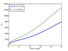
(a) $C_{H}$

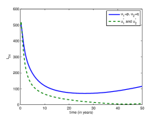
(b) $I_{TH}$

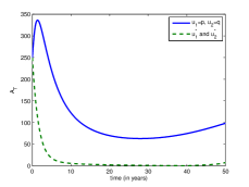
(c) $A_{T}$

Figure 2. Dynamics $C_{H}$, $I_{TH}$ and $A_{T}$ for cost functional (23), $\beta_{1}=0.6$, $\beta_{2}=0.1$, $W_{1}=W_{2}=50$ and parameter values from Table 2.

During approximately 40 years the optimal combination of the fractions of individuals $I_{TH}$ that take HIV and TB treatments simultaneously and only TB treatment is around $0.5$ and $0.46$, respectively, see Figure 3 (a) and (b). In Figure 3 (c) we observe that the extremal controls satisfy the restriction (22).

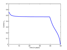
(a) $u_{1}^{*}$

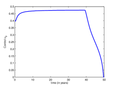
(b) $u_{2}^{*}$

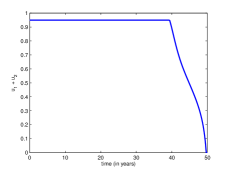
(c) $u_{1}^{*}+u_{2}^{*}$

Figure 3. Extremal controls $u_{1}^{*}$ and $u_{2}^{*}$ for cost functional (23), $\beta_{1}=0.6$, $\beta_{2}=0.1$, $W_{1}=W_{2}=50$ and parameter values from Table 2.

Figure 4. Total population $N$ for cost functional (23), $\beta_{1}=0.6$, $\beta_{2}=0.1$, $W_{1}=W_{2}=50$ and parameter values from Table 2.

At the end of 50 years, the number of TB and AIDS induced deaths reduces 5% when the controls $u_{1}^{*}$, $u_{2}^{*}$ are applied, see Figure 4. Since the HIV treatments have higher costs than TB treatment, we can consider that the weight constant $W_{1}$ associated to the control $u_{1}$ takes greater values than $W_{2}$. In this case, the fraction of individuals that take TB and HIV treatment $u_{1}^{*}$ decreases and the fraction of individuals that take only TB treatment increases, compared to the previous case $W_{1}=W_{2}=50$, but the associated extremal dynamics $C_{H}^{*}$, $I_{H}^{*}$ and $A_{T}^{*}$ behave similarly to the ones in the case $W_{1}=W_{2}=50$, see Figure 5.

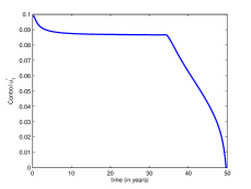
(a) $u_{1}^{*}$

(b) $u_{2}^{*}$

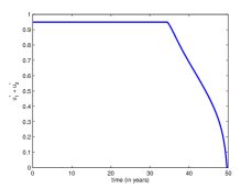
(c) $u_{1}^{*}+u_{2}^{*}$

Figure 5. Extremal controls $u_{1}^{*}$ and $u_{2}^{*}$ for cost functional (23), $\beta_{1}=0.6$, $\beta_{2}=0.1$, $W_{1}=500$, $W_{2}=50$ and parameter values from Table 2.

The extremal controls in Figure 5 (a) and (b) are not intuitive, since the fraction of individuals that take both HIV and TB treatments is very low. If we assume that our aim is to minimize the cost functional

$$J_{1}(u_{1}(\cdot),u_{2}(\cdot))=\int_{0}^{T}\left[A(t)+A_{T}(t)+\frac{W_{1}}{2}u_{1}^{2}(t)+\frac{W_{2}}{2}u_{2}^{2}(t)\right]dt,$$ (27)

with $T=10$ years and no disease induced deaths ($d_{T}=d_{TA}=d_{A}=0$), that is, we wish to minimize the number of individuals that have only AIDS $A$ and have both AIDS and TB diseases $A_{T}$, the extremal controls behave in a more intuitive way. Since we assume that there is no disease induced deaths we consider that is more adequate to consider $T=10$ instead of $T=50$ years. Moreover, is this case, the total population is constant. We observe that the fraction of individuals that take both HIV and TB treatment $u_{1}^{*}$ takes the maximum value for more than 7 years, and during this time the extremal control $u_{2}^{*}$ vanishes, see Figure 6.

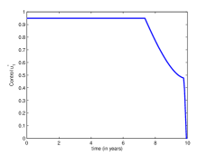
(a) $u_{1}^{*}$

(b) $u_{2}^{*}$

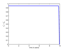
(c) $u_{1}^{*}+u_{2}^{*}$

Figure 6. Extremal controls $u_{1}^{*}$ and $u_{2}^{*}$ for cost functional $J_{1}$, with $\beta_{1}=0.6$, $\beta_{2}=0.1$, $W_{1}=W_{2}=50$ and parameter values from Table 2.

In this case, we compare the behavior of the dynamics $A$, $A_{T}$, $I_{TH}$ and $C_{H}$ for the following cost functionals $J_{1}$, $J_{2}$ and $J_{3}$, with $W_{1}=W_{2}=50$, where

$$J_{2}(u_{1}(\cdot))=\int_{0}^{T}\left[A(t)+A_{T}(t)+\frac{W_{1}}{2}u_{1}^{2}(t)\right]dt,$$ (28)

$$J_{3}(u_{2}(\cdot))=\int_{0}^{T}\left[A(t)+A_{T}(t)+\frac{W_{2}}{2}u_{2}^{2}(t)\right]dt,$$ (29)

that is, when both controls $u_{1}$ and $u_{2}$ are applied simultaneously, or are applied separately.

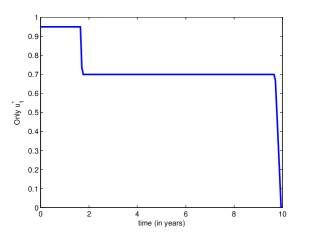
(a) $u_{1}$

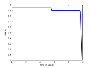
(b) $u_{2}$

Figure 7. Extremal controls when $u_{1}$ and $u_{2}$ are applied separately.

The number of individuals with only AIDS, $A$, is lower for cost functional $J_{1}$ and with extremal controls given by $u_{1}^{*}$ and $u_{2}^{*}$ in Figure 6 (a) and (b), see Figure 8 (a). However, this is not the best strategy for the reduction of the number of individuals with both AIDS and TB diseases, $A_{T}$. In this case, the best strategy is to apply only control $u_{1}$ where $u_{1}$ takes the values given in Figure 7, see Figure 8 (b). The best strategy for the reduction of the total number of individuals with only AIDS and with both AIDS and TB, $A+A_{T}$, during the first six years is the one associated to the cost functional $J_{2}$, that is, apply only control $u_{1}^{*}$ (see Figure 7 (a)) and after six years the best strategy is to apply simultaneously both controls $u_{1}^{*}$ and $u_{2}^{*}$ given by Figure 6.

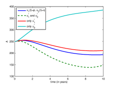
(a) $A$

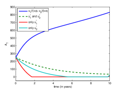
(b) $A_{T}$

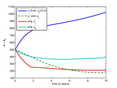
(c) $A+A_{T}$

Figure 8. Dynamics $A$, $A_{T}$ and $A+A_{T}$ for cost functionals $J_{1}$, $J_{2}$, $J_{3}$ and $u_{1}=p=0.1$, $u_{2}=q=0.3$, with $\beta_{1}=0.6$, $\beta_{2}=0.1$, $W_{1}=W_{2}=50$ and parameter values from Table 2.

In Figure 9 we observe that the implementation of controls $u_{1}$ and $u_{2}$ simultaneously or separately, contribute to the reduction of the number of individuals infected with HIV and TB, $I_{TH}$, and increase the number of individuals that remain in the class $C_{H}$, that is, the HIV infection does not evolve to AIDS disease. In this case, the strategy of treating only TB for the individuals in the class $I_{TH}$ does not allow equal or better results on the reduction of individuals in the class $I_{TH}$, which happens in the situation described in Figure 5 for the case $W_{1}=500$ and $W_{2}=50$.

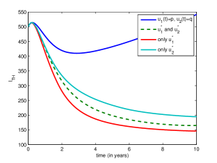
(a) $I_{TH}$

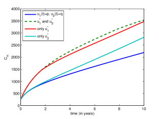
(b) $C_{H}$

Figure 9. Dynamics $I_{TH}$ and $C_{H}$ for cost functionals $J_{1}$, $J_{2}$, $J_{3}$ and $u_{1}=p=0.1$, $u_{2}=q=0.3$, with $\beta_{1}=0.6$, $\beta_{2}=0.1$, $W_{1}=W_{2}=50$ and parameter values from Table 2.

Symbol	Description	Value	References
$N$	Total population	variable
$N(0)$	Initial population	$30000$
$\Lambda$	Recruitment rate	$430$
$\mu$	Natural death rate	$1/70$
$\beta_{1}$	TB transmission rate	variable
$\beta_{2}$	HIV transmission rate	variable
$\eta_{C}$	Modification parameter	$0.9$
$\eta_{A}$	Modification parameter	$1.05$
$k_{1}$	Rate at which individuals leave $L_{T}$ class by becoming infectious	$1/2$	[7, 21]
$\tau_{1}$	TB treatment rate for $L_{T}$ individuals	$2$	[7, 21]
$\tau_{2}$	TB treatment rate for $I_{T}$ individuals	$1$	[7, 21]
$\beta^{\prime}_{1}$	Modification parameter	$0.9$
$d_{T}$	TB induced death rate	$1/10$	[7]
$\delta$	Modification parameter	$1.03$
$\psi$	Modification parameter	$1.07$
$\phi$	HIV treatment rate for $I_{H}$ individuals	$1$
$\rho_{1}$	Rate at which individuals leave $I_{H}$ class to $A$	$0.1$
$\alpha_{1}$	AIDS treatment rate	$0.33$	[3]
$\omega_{1}$	Rate at which individuals leave $C_{H}$ class	$0.09$
$d_{A}$	AIDS induced death rate	$0.3$
$\rho_{2}$	Rate at which individuals leave $I_{TH}$ class	$1$
$p$	Fraction of $I_{TH}$ individuals that take HIV and TB treatment	$0.1$
$q$	Fraction of $I_{TH}$ individuals that take only TB treatment	$0.3$
$\tau_{3}$	Rate at which individuals leave $L_{TH}$ class	$2$
$k_{2}$	Rate at which individuals leave $L_{TH}$ class by becoming TB infectious	$1.3\,k_{1}$
$r$	Fraction of $L_{TH}$ individuals that take HIV and TB treatment	$0.3$
$\beta^{\prime}_{2}$	Modification parameter	$1.1$
$\omega_{2}$	Rate at which individuals leave $R_{H}$ class	$0.15$
$\alpha_{2}$	HIV treatment rate for $A_{T}$ individuals	$0.33$
$d_{TA}$	AIDS-TB induced death rate	$0.33$

Table 2. Parameters of the TB-HIV/AIDS model.

7. Final comments and future work

Our numerical results only give extremals and no claims about optimality are made. As future work, it would be interesting to verify optimality by using second order optimality conditions and addressing properly the issue of conjugate points. For that, one needs to extend the theory underlying the computation of conjugate points and verification of optimality as developed in [38, Section 5.3] and [39].

References

- [1] AVERT, HIV & AIDS Information from AVERT.org, http://www.avert.org/worldwide-hiv-aids-statistics.htm#sthash.YzzqcNUT.dpuf
- [2] (MR2425430) [10.1007/s00285-008-0177-z] N. Bacaër, R. Ouifki, C. Pretorius, R. Wood, B. Williams, Modeling the joint epidemics of TB and HIV in a South African township, J. Math. Biol. 57, 557–593 (2008).
- [3] (MR2544634) [10.1007/s11538-009-9423-9] C. P. Bhunu, W. Garira and Z. Mukandavire, Modeling HIV/AIDS and tuberculosis coinfection, Bul. Math. Biol. 71, 1745–1780 (2009).
- [4] (MR3181992) [10.3934/mbe.2014.11.761] M. H. A. Biswas, L. T. Paiva and MdR de Pinho, A SEIR model for control of infectious diseases with constraints, Mathematical Biosciences and Engineering, Vol. 11, No. 4, 761–784 (2014).
- [5] (MR2718356) [10.1007/s11071-010-9683-9] S. Bowong, Optimal control of the transmission dynamics of tuberculosis, Nonlinear Dynam. 61, no. 4, 729–748 (2010).
- [6] (MR0635782) J. Carr, Applications centre manifold theory, Springer-Verlag, New-York (1981).
- [7] (MR1479331) [10.1007/s002850050069] C. Castillo-Chavez and Z. Feng, To treat or not to treat: The case of tuberculosis, J. Math. Biol. 35, no. 6, 629–656 (1997).
- [8] (MR1938888) [10.1007/978-1-4757-3667-0_13] C. Castillo-Chavez, Z. Feng and W. Huang, On the computation its role on global stability, Mathematical approaches for emerging and re-emerging infectious diseases. IMA, 125, 229–250 (2002).
- [9] (MR2130673) [10.3934/mbe.2004.1.361] C. Castillo-Chavez and B. Song, Dynamical models of tuberculosis and their applications, Math. Biosc. Engrg. 1, no. 2, 361–404 (2004).
- [10] (MR0688142) L. Cesari, Optimization — Theory and Applications. Problems with Ordinary Differential Equations, Applications of Mathematics 17, Springer-Verlag, New York, 1983.
- [11] [10.1016/S0140-6736(08)61115-0] P. W. David, G. L. Matthew, E. G. Andrew, A. C. David and M. K. John, Relation between HIV viral load and infectiousness: A model-based analysis, The Lancet 372, no. 9635, 314–320 (2008).
- [12] [10.1016/S0140-6736(13)61809-7] S. G. Deeks, S. R. Lewin, D. V. Havlir, The end of AIDS: HIV infection as a chronic disease, The Lancet, Vol. 382, Issue 9903, 1525–1533 (2013).
- [13] (MR1882991) O. Diekmann, J. A. P. Heesterbeek, Mathematical epidemiology of infectious diseases, Wiley Series in Mathematical and Computational Biology, Wiley, Chichester, 2000.
- [14] (MR1057044) [10.1007/BF00178324] O. Diekmann, J. A. P. Heesterbeek, J. A. J. Metz, On the definition and the computation of the basic reproduction ratio in models for infectious diseases in heterogeneous populations, J. Math. Biol. 28, no. 4, 365–382 (1990).
- [15] (MR2844653) [10.1155/2011/398476] Y. Emvudu, R. Demasse, D. Djeudeu, Optimal control of the lost to follow up in a tuberculosis model, Comput. Math. Methods Med. 2011 (2011), Art. ID 398476, 12 pp.
- [16] (MR0454768) W. H. Fleming, R. W. Rishel, Deterministic and Stochastic Optimal Control, Springer Verlag, New York, 1975.
- [17] R. Fourer, D. M. Gay, B. W. Kernighan, AMPL: A Modeling Language for Mathematical Programming, Duxbury Press, Pacific Grove, CA, 1993.
- [18] [10.1086/651492] H. Getahun, C. Gunneberg, R. Granich and P. Nunn, HIV infection-associated tuberculosis: The epidemiology and the response, Clin. Infect. Dis. 50 (Suppl 3), S201–S207 (2010).
- [19] (MR2487575) K. Hattaf, M. Rachik, S. Saadi, Y. Tabit, N. Yousfi, Optimal control of tuberculosis with exogenous reinfection, Appl. Math. Sci. (Ruse) 3, no. 5-8, 231–240 (2009).
- [20] (MR1814049) [10.1137/S0036144500371907] H. W. Hethcote, The mathematics of infectious diseases, SIAM Rev. 42 (4), 599–653 (2000).
- [21] (MR1921233) [10.3934/dcdsb.2002.2.473] E. Jung, S. Lenhart, Z. Feng, Optimal control of treatments in a two-strain tuberculosis model, Discrete Contin. Dyn. Syst. Ser. B 2, no. 4, 473–482 (2002).
- [22] [10.1006/tpbi.1998.1382] D. Kirschner, Dynamics of co-infection with M. tuberculosis and HIV-1, Theor. Pop. Biol. 55, no. 1, 94–109 (1999).
- [23] (MR1479338) [10.1007/s002850050076] D. Kirschner, S. Lenhart, S. Serbin, Optimal control of the chemotherapy of HIV, J. Mathematical Biology 35, 775–792 (1996).
- [24] [10.1128/CMR.00042-10] C. K. Kwan and J. D. Ernst, HIV and tuberculosis: A deadly human syndemic, Clin. Microbiol. Rev. 24, no. 2, 351–376 (2011).
- [25] (MR0984861) V. Lakshmikantham, S. Leela, and A.A Martynyuk, Stability Analysis of Nonlinear Systems, Marcel Dekker, Inc., New York and Basel (1989).
- [26] (MR3012899) [10.3934/proc.2011.2011.981] U. Ledzewicz, H. Schättler, On optimal singular controls for a general SIR-model with vaccination and treatment, Discrete Contin. Dyn. Syst., Dynamical systems, differential equations and applications. 8th AIMS Conference. Suppl. Vol. II, 981–990 (2011).
- [27] (MR2316829) S. Lenhart, J. T. Workman, Optimal control applied to biological models, Chapman & Hall/CRC, Boca Raton, FL, 2007.
- [28] (MR2604714) [10.1080/08898480903467241] G. Magombedze, W. Garira, and E. Mwenje, Modeling the TB/HIV-1 Co-Infection and the Effects of Its Treatment, Math. Pop. Studies, 17: 1, 12–64 (2010).
- [29] (MR2597074) [10.3846/1392-6292.2009.14.483-494] G. Magombedze, Z. Mukandavire, C. Chiyaka and G. Musuka, Optimal control of a sex structured HIV/AIDS model with condom use, Mathematical Modelling and Analysis 14:4, 483–494 (2009).
- [30] (MR2195099) [10.1080/13926292.2005.9637287] R. Naresh and A. Tripathi, Modelling and analysis of HIV-TB co-infection in a variable size population, Math. Model. Anal. 10, 275–286 (2005).
- [31] (MR0166037) L. Pontryagin, V. Boltyanskii, R. Gramkrelidze, E. Mischenko, The Mathematical Theory of Optimal Processes, Wiley Interscience, 1962.
- [32] PROPT, Matlab Optimal Control Software (DAE, ODE), http://tomdyn.com
- [33] (MR2719552) [10.1016/j.mcm.2010.06.034] H. S. Rodrigues, M. T. T. Monteiro, D. F. M. Torres, Dynamics of dengue epidemics when using optimal control, Math. Comput. Modelling 52, no. 9-10, 1667–1673 (2010). arXiv:1006.4392
- [34] (MR2878568) [10.1080/00207160.2011.554540] H. S. Rodrigues, M. T. T. Monteiro, D. F. M. Torres, A. Zinober, Dengue disease, basic reproduction number and control, Int. J. Comput. Math. 89, no. 3, 334–346 (2012). arXiv:1103.1923
- [35] (MR3266821) [10.1007/s11538-014-0028-6] P. Rodrigues, C. J. Silva, D. F. M. Torres, Cost-effectiveness analysis of optimal control measures for tuberculosis, Bull. Math. Biol. 76, no. 10, 2627–2645 (2014). arXiv:1409.3496
- [36] (MR2591215) [10.3934/mbe.2009.6.815] L. W. Roeger, Z. Feng and C. Castillo-Chavez, Modeling TB and HIV co-infections, Math. Biosc. and Eng. 6, no. 4, 815–837 (2009).
- [37] W. N. Rom, S. B. Markowitz, Environmental and Occupational Medicine, Lippincott Williams & Wilkins (2007).
- [38] (MR2798273) [10.1007/978-1-4614-3834-2] H. Schättler and U. Ledzewicz, Geometric optimal control, Springer, New York, 2012.
- [39] (MR3275020) [10.3934/dcdsb.2014.19.2657] H. Schättler, U. Ledzewicz, H. Maurer, Sufficient conditions for strong local optimality in optimal control problems with -type objectives and control constraints, Discrete Contin. Dyn. Syst. Ser. B 19, no. 8, 2657–2679 (2014).
- [40] (MR2401283) [10.3934/mbe.2008.5.145] O. Sharomi, C.N. Podder, A.B. Gumel and B. Song, Mathematical analysis of the transmission dynamics of HIV/TB coinfection in the presence of treatment, Math. Biosc. Eng. 5, no. 1, 145–174 (2008).
- [41] (MR2970904) [10.3934/naco.2012.2.601] C. J. Silva and D. F. M. Torres, Optimal control strategies for tuberculosis treatment: a case study in Angola, Numer. Algebra Control Optim. 2, no. 3, 601–617 (2012). arXiv:1203.3255
- [42] (MR3101449) [10.1016/j.mbs.2013.05.005] C. J. Silva and D. F. M. Torres, Optimal control for a tuberculosis model with reinfection and post-exposure interventions, Math. Biosci. 244, no. 2, 154–164 (2013). arXiv:1305.2145
- [43] K. Styblo, State of art: epidemiology of tuberculosis, Bull. Int. Union Tuberc. 53, 141–152 (1978).
- [44] (MR1205534) [10.1137/0524026] H.R. Thieme, Persistence under relaxed point-dissipaty (with applications to an epidemic model), SIAM. J. Math. Anal. Appl. 24, 407–435 (1993).
- [45] UNAIDS, Global report: UNAIDS report on the global AIDS epidemic 2013, Geneva, World Health Organization (2013).
- [46] (MR1950747) [10.1016/S0025-5564(02)00108-6] P. van den Driessche and J. Watmough, Reproduction numbers and subthreshold endemic equilibria for compartmental models of disease transmission, Math. Biosc. 180, 29–48 (2002).
- [47] (MR2195616) [10.1007/s10107-004-0559-y] A. Wächter, L. T. Biegler, On the implementation of an interior-point filter line-search algorithm for large-scale nonlinear programming, Math. Program. 106, no. 1, Ser. A, 25–57 (2006).
- [48] WHO, Global tuberculosis report 2013, Geneva, World Health Organization (2013).
- [49] WHO, Tuberculosis, Fact sheet no. 104, http://www.who.int/mediacentre/factsheets/fs104/en, Updated October 2014.