Frequency comb generation for wave transmission through the nonlinear dimer

Abstract

We study dynamical response of a nonlinear dimer to a symmetrically injected monochromatic wave. We find a domain in the space of frequency and amplitude of the injected wave where all stationary solutions are unstable. In this domain scattered waves carry multiple harmonics with equidistantly spaced frequencies (frequency comb effect). The instability is related to a symmetry protected bound state in the continuum whose response is singular as the amplitude of the injected wave tends to zero.

I Introduction

A nonlinear quantum dimer represents the simplest realization of the discrete nonlinear Schrödinger equation and has attracted much interest for a long time Eilbeck ; Campbell ; Tsironis ; Kenkre0 ; Kenkre ; Tsironis1 ; Molina ; Miros ; Pickton ; Xu . The interest is related to the phenomenon of symmetry breaking (self-trapping) Eilbeck ; Campbell ; Molina ; Berstein . On the other hand, non-trivial time-dependent solutions were found in the nonlinear dimer Eilbeck ; Campbell ; Tsironis ; Kenkre0 ; Kenkre ; Tsironis1 ; Pickton .

The observation of these remarkable properties of the closed nonlinear dimer implies application of a probing wave that opens the dimer. Respectively, temporal equations describing the open nonlinear dimer become non-integrable which constitutes the main difference between the closed and open nonlinear dimers. As dependent on the way of opening the transmission through nonlinear dimer was studied in Refs. Maes1 ; Maes2 ; Miros2 ; BPS ; Brazhnyi ; Miros3 ; Shapira ; T ; Maksimov ; Xu-Miros ; Barashenkov where the phenomenon of symmetry breaking was reported. What is interesting there is a domain in the space of frequency and amplitude of injected wave where stable stationary solutions of the temporal equations do not exist BPS ; Maksimov . Thus one can expect that the dynamical response of the nonlinear dimer will display features which can not be described by the stationary scattering theory. In particular injection of a monochromatic symmetric wave into the nonlinear plaquette gives rise to emission of anti-symmetric satellite waves with frequencies different from the frequency of the incident wave Maksimov . This phenomenon is known as frequency comb (FC) generation and is widely studied in various linear and nonlinear systems Science ; Lushui ; Abrams . The FC generation can be interpreted as a modulational instability of the continuous-wave pump mode Matsko revealed even in a single off-channel nonlinear cavity Hansson . In this paper we show that illumination of the nonlinear dimer with a monochromatic wave in the domain of instability gives rise to FC generation.

II Coupled mode theory equations

The nonlinear dimer can be realized in 2D photonic crystal in the form of coupled microcavities based on two identical dielectric defect rods with the Kerr effect BPS as shown in Fig. 1 (a).

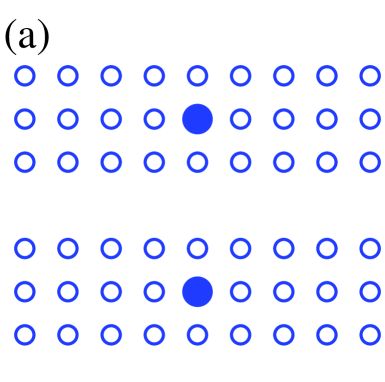
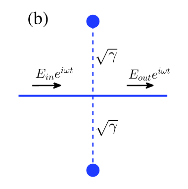
Figure 1: (a) Two identical microcavities made from a Kerr media marked by filled circles are inserted into the square lattice photonic crystal of dielectric rods. The 1D waveguide is formed by extraction of a linear chain. (b) Two nonlinear sites marked by filled circles are positioned symmetrically relative to waveguide and form open nonlinear dimer.

Taking the radii of the rods small enough we can present each rod by a single site variable $A_{j},j=1,2$ disregarding space inhomogeneity of electromagnetic field in the rods. In terms of the eigenfunctions of the Maxwell equations for each microcavity it means that only the monopole mode with the eigenfrequency $\omega_{0}$ resides in the photonic crystal waveguide propagation band and thereby is relevant in the scattering. For simplicity we disregard the dispersion properties of the waveguide and write for the dimer illuminated by light with the amplitude $E_{in}$ and frequency $\omega$ the following temporal coupled mode theory (CMT) equations Haus ; Suh ; BPS

$$-i\dot{A_{1}}=(\omega_{0}+\lambda|A_{1}|^{2})A_{1}+uA_{2}+i\gamma(A_{1}+A_{2})-i\sqrt{\gamma}E_{in}e^{i\omega t},$$

$$-i\dot{A_{2}}=(\omega_{0}+\lambda|A_{2}|^{2})A_{2}+uA_{1}+i\gamma(A_{1}+A_{2})-i\sqrt{\gamma}E_{in}e^{i\omega t}.$$ (1)

Here the terms $\lambda|A_{j}|^{2}A_{j},j=1,2$ account for the Kerr effect of each microcavity, the term $\sqrt{\gamma}$ is responsible for the coupling of the off-channel cavity with the waveguide. The monopole mode of each cavity is localized within a few lattice units Joanbook . If the cavities are positioned far from waveguide we can neglect direct coupling $u$ between them. However even for this case the open nonlinear dimer remains cardinally different from the case of the closed dimer because of the interaction between the cavities via the continuum. For simplicity we consider the case $u=0$. The amplitude of the transmitted wave is given by the following equation Suh ; BPS

$$E_{out}=E_{in}-\sqrt{\gamma}(a_{1}+a_{2})$$ (2)

where $A_{j}(t)=a_{j}(t)e^{i\omega t}$. The open dimer governed by the CMT equations (II) is shown in Fig. 1 (b).

Assuming that the solution is stationary $a_{j}(t)=a_{j0}=const$ the CMT equations (II) are simplified to

$$(\nu+\lambda|a_{10}|^{2})a_{10}+i\gamma(a_{10}+a_{20})-i\sqrt{\gamma}E_{in}=0\,$$

$$(\nu+\lambda|a_{20}|^{2})a_{20}+i\gamma(a_{10}+a_{20})-i\sqrt{\gamma}E_{in}=0\,$$ (3)

where $\nu=\omega_{0}-\omega$. As the input amplitude $E_{in}$ increases the system bifurcates from the symmetry preserving solution $a_{10}=a_{20}$ to the symmetry breaking solution $I_{1}\neq I_{2},\theta_{1}-\theta_{2}=0,\pi$ where $a_{j0}=\sqrt{I_{j}}\exp(i\theta_{j}),j=1,2$ similar to the closed nonlinear dimer Eilbeck ; Tsironis ; Kenkre . However in contrast to the closed nonlinear dimer the open dimer can also transit into the phase symmetry breaking solution with $I_{1}=I_{2}$ but $\theta_{1}-\theta_{2}\neq 0,\pi$ BPS ; Maksimov .

III instability of stationary solutions

Numerical analysis of stability of the stationary solutions revealed a domain in the space of parameters $\omega$ and $E_{in}$ where all stationary solutions are unstable BPS . Similar result was found in the open plaquette of four nonlinear cites Maksimov . In this section we find the domain of instability of stationary solutions of temporal equations (II) analytically.

To examine the stability of solutions of Eq. (II) we apply a standard small perturbation technique Litchinitser ; Cowan :

$$a_{j}(t)=a_{j0}+(x_{j}+iy_{j})e^{\mu t},~{}~{}j=1,2,$$ (4)

where the second term in Eq. (4) is considered to be small. For the symmetry preserving solutions we have from Eq. (II)

$$a_{10}=a_{20}=A_{0}=\frac{i\sqrt{\gamma}E_{in}}{\nu+\lambda I_{0}+2i\gamma}$$ (5)

where according to Eq. (II)

$$I_{0}[(\nu+\lambda I_{0})^{2}+4\gamma^{2}]=\gamma E_{in}^{2},$$ (6)

and $I_{0}=|A_{0}|^{2}$. Substituting (4) into Eq. (II) we obtain the following system of algebraic equations

$$-(\mu+2\lambda Re(A_{0})Im(A_{0}))(x_{1}-x_{2})=(\nu+\lambda I_{0}+2\lambda Im(A_{0})^{2})(y_{1}-y_{2}),$$

$$(\mu-2\lambda Re(A_{0})Im(A_{0}))(y_{1}-y_{2})=(\nu+\lambda I_{0}+2\lambda Re(A_{0})^{2})(x_{1}-x_{2}),$$ (7)

and

$$-(\mu+2\gamma+2\lambda Re(A_{0})Im(A_{0}))(x_{1}+x_{2})=(\nu+\lambda I_{0}+2\lambda Im(A_{0})^{2}(y_{1}+y_{2})$$

$$(\mu+2\gamma-2\lambda Re(A_{0})Im(A_{0}))(y_{1}+y_{2})=(\nu+\lambda I_{0}+2\lambda Re(A_{0})^{2})(x_{1}+x_{2}).$$ (8)

For Eq. (III) we obtain the eigenvalues

$$\mu^{2}=-(\nu+\lambda I_{0})(\nu+3\lambda I_{0}).$$ (9)

The equation $\mu=0$ defines the boundary where the symmetry preserving family of the stationary solutions becomes unstable Cowan . From Eq. (9) we obtain equations $\nu+\lambda I_{c}=0$ and $\nu+3\lambda I_{c}=0$. Substituting these values of $I_{c}$ into Eq. (6) we obtain for the boundaries of the domain where stable stationary solutions do not exist

$$E_{in}^{2}=-\frac{4\gamma\nu}{\lambda},$$

$$E_{in}^{2}=-\frac{4\nu}{3\lambda\gamma}[\nu^{2}/9+\gamma^{2}].$$ (10)

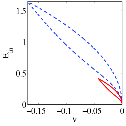
Figure 2: (Color online) Domain in space of physical parameters $\nu=\omega_{0}-\omega$ and $E_{in}$ where all stationary solutions are unstable for $\gamma=0.01$ (red solid line) and $\gamma=0.04$ (blue dash line). Other parameters are $\omega_{0}=1,\lambda=0.01$.

The domains of instability of stationary solutions are shown in Fig. 2. Eq. (III) does not give contribution into the domain of instability. Also numerical analysis of the stability has shown that the symmetry breaking and phase symmetry breaking solutions fall into the same domain of stability as the symmetry preserving solution.

IV numerical solutions of nonlinear temporal CMT equations

Substituting $A_{j}(t)=a_{j}(t)\exp(i\omega t)$ into the temporal CMT equations (II) we obtain

$$-i\dot{a_{1}}=(\nu+\lambda|a_{1}|^{2})a_{1}+i\gamma(a_{1}+a_{2})-i\sqrt{\gamma}E_{in},$$

$$-i\dot{a_{2}}=(\nu+\lambda|a_{2}|^{2})a_{2}+i\gamma(a_{1}+a_{2})-i\sqrt{\gamma}E_{in}.$$ (11)

One can see that the solutions possess a symmetry with the half period time shift corresponding to the permutation of the sites

$$a_{1}(t+T/2)=a_{2}(t),a_{2}(t+T/2)=a_{1}(t).$$ (12)

Indeed, after time shift $t\rightarrow t+T/2$ in the first equation in (IV) we obtain the second equation using Eq. (12) and the periodicity of the solutions. Thus, the system of equations (IV) is reduced to one temporal equation

$$-i\dot{a_{j}}=(\nu+\lambda|a_{j}(t)|^{2})a_{j}(t)+i\gamma(a_{j}(t)+a_{j}(t+T/2))-i\sqrt{\gamma}E_{in}.$$ (13)

Nevertheless the symmetry (12) does not allow to solve Eq. (13) because of unknown period $T$ which strongly depends on the intensity of the injected wave. In Fig. 3 and Fig. 4 we present the results of numerical simulations

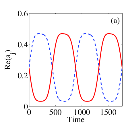
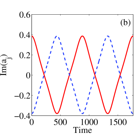
Figure 3: (Color online) Time evolution of site amplitudes $A_{j}(t),j=1,2$, real and imaginary parts for $E_{in}=0.1,\nu=-0.001,\gamma=0.04,\lambda=0.01$.

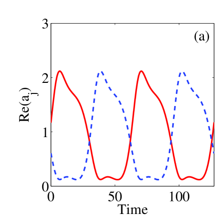
Figure 4: (Color online) The same as in Fig. 3 but for the parameters $E_{in}=0.4,\nu=-0.02,\gamma=0.04,\lambda=0.01$.

of Eq. (IV) in the domain of unstable stationary solutions which demonstrate the symmetry (12). Fig. 4 also demonstrates rachet effect due to absence of the time reversal symmetry in the open dimer. We chose the parameters listed in caption of Fig. 3 and Fig. 4 guided by the data on photonic crystal microcavities from Ref. BPS .

In order to compare the results with the closed dimer Ref. Eilbeck we present trajectories projected onto the modulus $|a_{j}|$ and phase difference $\Delta\theta$ between cavities in Fig. 5 (a). Although for a small injected amplitude $E_{in}$ the trajectories look similar to those shown in Ref. Eilbeck however with the growth of $E_{in}$ the trajectories become asymmetrical relative to $\Delta\theta\rightarrow-\Delta\theta$. The trajectories projected onto the real and imaginary parts of the amplitudes $a_{j}(t)$ demonstrate the most striking difference between the closed and open nonlinear dimer as shown in Fig. 5 (b). While for the closed dimer the trajectories form circles centered at the origin of the coordinate system (they are not shown in Fig. 5 (b)) the trajectories of the open dimer are shifted relative to the coordinate origin. Phase transformation of the injected wave $E_{in}\rightarrow E_{in}e^{i\alpha}$ rotates the trajectories in Fig. 5 (b) by the same angle $\alpha$.

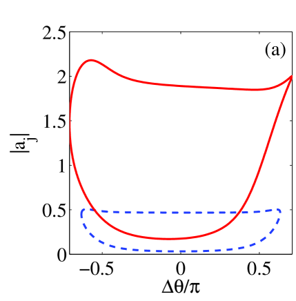
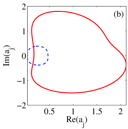
Figure 5: (Color online) (a) Trajectories projected onto $|a_{j}|$ and phase difference $\Delta\theta=\theta_{1}-\theta_{2}$ and (b) real and imaginary parts of amplitudes $a_{j}(t),j=1,2$ for different points in the domain of instability: $E_{in}=0.1,\nu=-0.001$ (blue dash line) and $E_{in}=0.4,\nu=-0.02$ (red solid line). Other parameters are $\omega_{0}=1,\gamma=0.04,\lambda=0.01$.

It is clear that such a complicated time behavior of the amplitudes will reflect at the transmitted wave according to Eq. (2). Fig. 6 shows the Fourier transformation of the transmitted wave

$$E_{out}(t)=\int dfE_{out}(f)\exp(ift)$$ (14)

that demonstrates sharp peaks spaced equidistantly, FC comb effect. In what follows we define the interval between the peaks of the Furrier transform $F_{out}(f)$ as the FC period $\Omega_{FC}$. One can see from Fig. 6 $|E_{out}(f)|\neq|E_{out}(-f)|$ that is a consequence of the rachet effect as seen from Fig. 4.

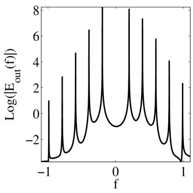
Figure 6: Fourier transform $E_{out}(f)$ of the transmitted wave in Log scale for the parameters listed in Fig. 4.

V the asymptotic evaluation of the frequency comb period

The reason for the cardinal difference between the closed and open nonlinear dimers is the symmetry of the system. Let us rewrite Eq. (IV) in terms of the eigenmodes of the closed linear dimer

$$-i\dot{a}_{s}=(\nu+\lambda[|a_{s}|^{2}+2|a_{a}|^{2}])a_{s}+\lambda a_{a}^{2}a_{s}^{*}+2i\gamma a_{s}-i\sqrt{\gamma}E_{in},$$

$$-i\dot{a}_{a}=(\nu+\lambda[|a_{a}|^{2}+2|a_{s}|^{2}])a_{a}+\lambda a_{s}^{2}a_{a}^{*}.$$ (15)

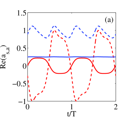
Figure 7: (Color online) Time evolution of real parts (a) and imaginary parts (b) of symmetric $a_{s}=\frac{1}{2}(a_{1}+a_{2})$ (blue lines) and antisymmetric mode $a_{a}=\frac{1}{2}(a_{1}-a_{2})$ (red lines) for $E_{in}=0.1,\nu=-0.001$ (solid lines) and $E_{in}=0.2,\nu=-0.02$ (dash lines). Other parameters are $\omega_{0}=1,\gamma=0.04,\lambda=0.01$.

where $a_{s,a}=\frac{1}{2}(a_{1}\pm a_{2})$ are the symmetric and antisymmetric eigenmodes of the dimer with the eigenfrequencies $\omega_{s,a}=\omega_{0}$.

Let us take temporarily the dimer linear. The design of the open dimer (Fig. 1) implies that the injected wave can probe only the symmetric mode with a Breit-Wigner response $a_{s}=i\sqrt{\gamma}E_{in}/(\nu+2i\gamma)$, while the antisymmetric mode remains hidden as seen from the CMT equations (V). It oscillates with the frequency $\nu$ however with the uncertain amplitude. That defines the antisymmetric mode $a_{a}$ as a symmetry protected bound state in the continuum photonics ; Moiseyev ; Segev ; Wei . Returning to the site amplitudes we therefore obtain

$$a_{j}=\frac{i\sqrt{\gamma}E_{in}}{\nu+2i\gamma}\pm ae^{i\nu t},~{}~{}j=1,2$$ (16)

making the time behavior of the site amplitudes of the linear dimer non stationary. This equation constitutes the time dependent contribution of the bound state in the continuum established for the stationary case in quantum mechanical ring and photonic crystal systems photonics .

The nonlinearity results in two effects. The first obvious result is that the resonance eigenfrequency $\nu+\lambda I_{0}$ of the symmetric mode is shifted proportional to $E_{in}^{2}$. That agrees with behavior of the instability domain at small $E_{in}$ as derived in Section III and shown in Fig. 2. The second effect is more sophisticated. For small $E_{in}$ the symmetric mode $a_{s}$ is almost constant while oscillations of the antisymmetric mode $a_{a}$ are dominant as shown in Fig. 7. As seen from the first equation in Eq. (V) the antisymmetric mode plays the role of a driving force for the mode $a_{s}$ via the the nonlinear term $\lambda a_{a}^{2}a_{s}^{*}$. Then if the frequency of the mode $a_{a}$ is $\Omega$ then the symmetric mode oscillates with double frequency $2\Omega$ as it is seen from the numerical solution in Fig. 7. Respectively, the transmitted wave carries the harmonics with the same frequency $2\Omega$ in accordance to Eq. (2).

In order to consider these nonlinear effects in the open nonlinear dimer we use the asymptotic methods by Bogoliubov and Mitropolsky Bogol . Eq. (V) can be rewritten as follows

$$i\dot{a}_{s}+(\nu+2i\gamma)a_{s}-i\sqrt{\gamma}E_{in}=\varepsilon F_{s}(a_{s},a_{a}),$$

$$i\dot{a}_{a}+\nu a_{a}=\varepsilon F_{a}(a_{s},a_{a})$$ (17)

where the parameter $\lambda$ is considered as a small parameter $\varepsilon$ and functions $F_{s,a}$ are polynomial functions of $a_{s,a}$ determined by Eq. (V). Then the solution up to the first order in $\varepsilon$ can be sought in the form

$$a_{s}=s_{0}(a,\phi)+\varepsilon s_{1}(a,\phi)$$

$$a_{a}=a_{0}(a,\phi)+\varepsilon a_{1}(a,\phi)$$ (18)

as functions of the amplitude $a$ and phase $\phi$. They are given by the following equations

$$\dot{a}=\varepsilon D_{1}(a)$$

$$\dot{\phi}=\nu+\varepsilon\Omega_{1}(a)$$ (19)

where $\nu$ is the frequency of oscillations at $\varepsilon=0$. Substitution of Eqs. (V), (V) and relation

$$\dot{a}_{s,a}=\dot{a}\frac{\partial a_{s,a}}{\partial a}+\dot{\phi}\frac{\partial a_{s,a}}{\partial\phi}.$$ (20)

into Eq. (V) gives the following equation at the zeroth order in parameter $\varepsilon$

$$s_{0}(a,\phi)=\frac{i\sqrt{\gamma}E_{in}}{\nu+2i\gamma},~{}~{}a_{0}(a,\phi)=a\exp(i\phi),$$ (21)

where the amplitude $a$ is undefined.

In the first order in $\varepsilon$ we obtain the following equations

$$-i\nu\frac{\partial s_{1}}{\partial\phi}=(\nu+2i\gamma)s_{1}+a_{0}^{2}s_{0}^{*}+(|s_{0}|^{2}+2a^{2})s_{0}$$

$$-i\nu\frac{\partial a_{1}}{\partial\phi}=\nu a_{1}+s_{0}^{2}a_{0}^{*}+(a^{2}+2|s_{0}|^{2})a_{0}+(iD_{1}-a\Omega_{1})\exp(i\phi).$$ (22)

One can expand

$$s_{1}(a,\phi)=\sum_{n}F_{s,n}(a)\exp(in\phi)$$ (23)

$$a_{1}(a,\phi)=\sum_{n}F_{a,n}(a)\exp(in\phi)$$ .

According to Ref. Bogol there is an uncertainty in choice of functions $s_{1}$ and $a_{1}$ that allows to exclude, for example, the first harmonic contributions $F_{s,1},F_{a,1}$ that gives the following equations

$$D_{1}(a)=0,~{}~{}\Omega_{1}(a)=a^{2}+2|s_{0}|^{2}.$$ (24)

Then, solutions of (V) are the following

$$s_{1}(a,\phi)=-\frac{|s_{0}|^{2}+2a^{2}}{\nu+2i\gamma}s_{0}+\frac{a^{2}}{\nu-2i\gamma}s_{0}^{*}\exp(2i\phi)$$

$$a_{1}(a,\phi)=-\frac{a}{2\nu}s_{0}^{2}\exp(-i\phi).$$ (25)

This equations show that the symmetric solution consists of even terms $n=0,\pm 2,\ldots$ in the expansion (23) while the antisymmetric solution consists of the odd terms $n=\pm 1,\pm 3,\ldots$. The higher orders in the small parameter holds these features. From Eq. (V) we have

$$\phi=\left(\nu+\lambda\left(a^{2}+2|s_{0}|^{2}\right)\right)t=\Omega_{a}t$$ (26)

which yields the FC period $\Omega_{FC}=2\Omega_{a}$ in the first order in $\lambda$ with the amplitude $a$ remaining undefined. This amplitude can be determined by the equation $\dot{a}=0$ in Eq. (V) if the injected amplitude $E_{in}$ is taken as a small parameter $\varepsilon$ in the perturbation approach. However that approach is successful only in the fourth order in $\varepsilon$ resulting in cumbersome equations. Therefore we estimate the amplitude $a$ averaging the numerical solution over time: $a=\langle a_{a}(t)\rangle$. The numerical result shown in Fig. 8 (a) is close to analytical result (26) in Fig. 8 (b) when the injected amplitude is small.

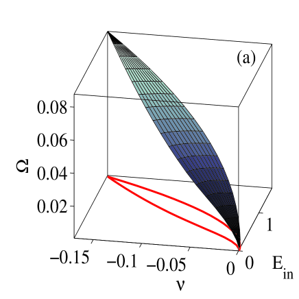
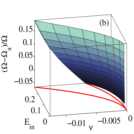
Figure 8: (Color online) (a) Period of harmonics $\Omega$ vs amplitude $E_{in}$ and frequency $\nu$ of injected monochromatic wave calculated numerically. (b) Difference between numerical data and analytical results given by Eq. (26). The parameters of the dimer are $\omega_{0}=1,\gamma=0.01,\lambda=0.01$. Below the domain of instability defined by Eq. (III) is shown by red lines.

Thus, the period of harmonics generated by the open nonlinear dimer can be effectively controlled by the injected amplitude.

Note, the reason for instability related to the bound state in the continuum preserves for $u\neq 0$ and what is more surprising even for different couplings $\gamma_{j},j=1,2$ of the sites with the injected wave. For this case the CMT equations (IV) will take the following form Suh

$$-i\dot{a_{1}}=(\nu+\lambda|a_{1}|^{2})a_{1}+i\gamma_{1}a_{1}+i\sqrt{\gamma_{1}\gamma_{2}}a_{2}-i\sqrt{\gamma_{1}}E_{in},$$

$$-i\dot{a_{2}}=(\nu+\lambda|a_{2}|^{2})a_{2}+i\sqrt{\gamma_{1}\gamma_{2}}a_{1}+i\gamma_{2}a_{2}-i\sqrt{\gamma_{2}}E_{in}.$$ (27)

By linear transformation

$$a_{1}=\sqrt{\gamma_{1}}(a_{s}+a_{a}),~{}~{}a_{2}=\sqrt{\gamma_{2}}(a_{s}-a_{a})$$ (28)

Eqs. (V) take the following form

$$-i\dot{a}_{s}=\nu a_{s}+\gamma_{+}\lambda[(|a_{s}|^{2}+2|a_{a}|^{2})a_{s}+a_{a}^{2}a_{s}^{*}]+\gamma_{-}\lambda[(|a_{a}|^{2}+2|a_{s}|^{2})a_{a}+a_{s}^{2}a_{a}^{*}]+2i(\gamma_{+}a_{s}+\gamma_{-}a_{a})-iE_{in},$$

$$-i\dot{a}_{a}=\nu a_{a}+\gamma_{-}\lambda[(|a_{s}|^{2}+2|a_{a}|^{2})a_{s}+a_{s}^{2}a_{s}^{*}]+\gamma_{+}\lambda[(|a_{a}|^{2}+2|a_{s}|^{2})a_{a}+a_{a}^{2}a_{s}^{*}+\gamma_{+}a_{s}^{2}a_{a}^{*}]$$ (29)

where $\gamma_{\pm}=(\gamma_{1}\pm\gamma_{2})/2$. One can see that similar to the former symmetric case $\gamma_{1}=\gamma_{2}$ the mode $a_{a}$ is coupled with the injected wave only through the nonlinear terms.

VI summary and discussion

In this paper we considered one of the simplest nonlinear open system, dimer whose closed counterpart is exactly integrable system Eilbeck . The term ”open” means that a linear waveguide is attached to the dimer to allow probing the dynamical properties of the dimer. Even in the case of decoupled ($u=0$) nonlinear sites they interact with each other through the continuum of the waveguide. In the framework of coupled mode theory we examined the stability of stationary solutions of Eq. (II) in the parametric space of frequency and amplitude of the probing wave. We found a domain where stable stationary solutions do not exist. First such domains were found in open nonlinear plaquette Maksimov together with the associated effect of frequency comb generation. In the present paper we showed a similar effect for scattering of a monochromatic wave by a nonlinear dimer.

The instability of the open nonlinear dimer is related to a symmetry protected bound state in the continuum. When the dimer is linear there were two eigenmodes, symmetric and antisymmetric. The symmetrical design of opening of the dimer (see Fig. 1) implies that the injected wave couples only with the symmetric mode while there is no direct coupling of the injected wave with the antisymmetric mode as seen from Eqs. (V). However owing to nonlinear terms in these equations the antisymmetric mode $a_{a}$ is coupled with injected wave through the symmetric mode $a_{s}$. Therefore the antisymmetric mode emerges in the response in the vicinity of the resonance $\nu=0$.

Numerical solution of the temporal coupled mode theory equations (V) demonstrates highly nonlinear behavior of the site amplitudes cardinally different from the dynamical behavior of the closed dimer in the instability domain. Time dependence of these amplitudes holds many harmonics whose frequencies are equidistantly spaced with the interval $\Omega$. This interval which defines the FC period $\Omega_{FC}=2\Omega$ was computed numerically and evaluated by the use of asymptotic methods Bogol to demonstrate an agreement as shown in Fig. 8. Respectively, the injected wave after scattering by the nonlinear dimer acquires these harmonics. The value $\Omega$ goes down with decreasing of the injected amplitude that opens a way of all-optical control of the harmonics.

- (1) J.C. Eilbeck, P.S. Lomdahl, and A.C. Scott, Physica 16D, 318 (1985).
- (2) V.M. Kenkre and D.K. Campbell, Phys. Rev. B34, 4959 (1986).
- (3) G.P. Tsironis and V.M. Kenkre, Phys. Lett. A127, 209 (1988).
- (4) V.M. Kenkre and H.-L. Wu, Phys. Rev B39, 6907 (1989); Phys. Lett. 135, 120 (1989).
- (5) V.M. Kenkre and M. Kuś, Phys. Rev. B49, 5956 (1994).
- (6) G.P. Tsironis, W.D. Deering and M.I. Molina, Physica D68, 135 (1993).
- (7) M.I. Molina, Mod. Phys. Lett. 13, 225 (1999).
- (8) A.E. Miroshnichenko, B.A. Malomed, and Yu.S. Kivshar, Phys. Rev. A84, 012123 (2011).
- (9) J. Pickton and H. Susanto, Phys. Rev. A88, 063840 (2013).
- (10) H. Xu, P.G. Kevrekidis, and A. Saxena, ”Generalized Dimers and their Stokes-variable Dynamics”, arXiv preprint arXiv:1404.4382, (2014).
- (11) L. Berstein, Physica D53, 240 (1991).
- (12) B. Maes, M. Soljaĉić, J.D. Joannopoulos, P. Bienstman, R. Baets, S.-P. Gorza, and M. Haelterman, Opt. Express, 14, 10678 (2006).
- (13) B. Maes, P. Bienstman, and R. Baets, Opt.Express 16, 3069 (2007).
- (14) A.E. Miroshnichenko, Phys. Rev.E 79, 026611 (2009).
- (15) E.N. Bulgakov, K.N. Pichugin, and A.F. Sadreev, Phys. Rev. B 83, 045109 (2011); J.Phys.: Cond. Mat. 23, 065304 (2011).
- (16) V.A. Brazhnyi and B.A. Malomed, Phys. Rev.A83, 053844 (2011).
- (17) A.E. Miroshnichenko, B.A. Malomed, and Yu.S. Kivshar, Phys. Rev.A84, 012123 (2011).
- (18) A. Shapira, N. Voloch-Bloch, B.A. Malomed, and A. Arie, J. Opt. Soc. AM. B28, 1481 (2011).
- (19) E.N. Bulgakov and A.F. Sadreev, Phys. Rev. B 84, 155304 (2011).
- (20) D.N. Maksimov and A.F. Sadreev, Phys. Rev. E88, 032901 (2013).
- (21) Yi Xu and A.E. Miroshnichenko, Phys. Rev. B89, 134306 (2014).
- (22) I.V. Barashenkov and M. Gianfreda, J. Phys. A: Math. Gen. 47, 282001 (2014).
- (23) T.J. Kippenberg, R. Holzwarth, and S.A. Diddams, Science 332, 555 (2011).
- (24) L.S. Cao, D.X. Qi, R.W. Peng, Mu Wang, and P. Schmelcher, Phys. Rev. Lett 112, 075505 (2014).
- (25) D.M. Abrams, A. Slawik, and K. Srinivasan, Phys. Rev. Lett. 112, 123901 (2014).
- (26) A.B. Matsko , A.A. Savchenkov, W. Liang, V.S. Ilchenko, D. Seidel, and L.Maleki, Opt. Lett. 36, 2845 (2011).
- (27) T.Hansson, D. Modotto, and S. Wabnitz, Phys. Rev. A88, 023819 (2013); Opt. Comm. 312, 134 (2014).
- (28) H.A.Haus, Waves and Fields in Optoelectronics (Prentice-Hall, N.Y., 1984).
- (29) W. Suh, Z. Wang, and S. Fan, IEEE J. of Quantum Electronics, 40, 1511 (2004).
- (30) J. Joannopoulos, R.D. Meade, and J. Winn, Photonic Crystals (Princeton University, Princeton, NJ, 1995).
- (31) N.M. Litchinitser, C.J. McKinstrie, C.M. de Sterke, and G.P. Agrawal, J. Opt. Soc. Am. B18, 45 (2001).
- (32) A.R. Cowan and J.F. Young, Phys.Rev.E68, 046606 (2003).
- (33) E.N. Bulgakov and A.F. Sadreev, Phys. Rev. B78, 075105 (2008).
- (34) N. Moiseyev, Phys. Rev. Lett. 102, 167404 (2009).
- (35) Y. Plotnik, et al, Phys. Rev. Lett. 107, 183901 (2011).
- (36) Chia Wei Hsu, et al, Nature, 499, 188 (2013).
- (37) E. N. Bulgakov, K.N. Pichugin, A. F. Sadreev, and I. Rotter, JETP Lett. 84 430 (2006).
- (38) N.N. Bogoliubov and Y.A. Mitropolsky Asymptotic Methods in the Theory of Non-Linear oscillations, Gordon and Breach, N.Y. 1962.