Subleading harmonic flows in hydrodynamic simulations of heavy ion collisions
Abstract
We perform a principal component analysis (PCA) of in event-by-event hydrodynamic simulations of Pb+Pb collisions at the Large Hadron Collider (LHC). The PCA procedure identifies two dominant contributions to the two-particle correlation function, which together capture 99.9% of the squared variance. We find that the subleading flow (which is the largest source of flow factorization breaking in hydrodynamics) is predominantly a response to the radial excitations of a third-order eccentricity. We present a systematic study of the hydrodynamic response to these radial excitations in 2+1D viscous hydrodynamics. Finally, we construct a good geometrical predictor for the orientation angle and magnitude of the leading and subleading flows using two Fourier modes of the initial geometry.
I Introduction
Two-particle correlation measurements in ultrarelativistic heavy ion collisions provide an extraordinarily detailed test of the hydrodynamic description of heavy ion events. Indeed, the measured two-particle correlations exhibit elliptic, triangular, and higher harmonic flows, which can be used to constrain the transport properties of the quark gluon plasma (QGP) produced in heavy ion collisions Heinz and Snellings (2013); Luzum and Petersen (2014). In hydrodynamic simulations of heavy-ion events, fluctuations in the initial state are propagated by the expansion dynamics of the QGP, and this expansion ultimately induces fluctuations in the momentum spectra of the produced particles. Thus, measurements of the momentum space fluctuations (or correlations) constrain the properties of the QGP expansion and the initial state. The purpose of the current paper is to classify and quantify the dominant momentum space fluctuations in (boost-invariant) event-by-event hydrodynamics, and then to optimally correlate these fluctuations in momentum space with specific fluctuations in the initial state geometry. The current paper is focused on triangular flow, since it is a strong signal and driven entirely by fluctuations Alver and Roland (2010). The corresponding studies of the other harmonics are postponed for future work.
Due to flow fluctuations the correlation matrix of event-by-event triangular flows, , in hydrodynamics does not factorize Gardim et al. (2013). Factorization breaking is quantified by the parameter ,
| (1) |
which must be less than unity when there are several statistically independent sources of triangular flow in the event sample Gardim et al. (2013). Factorization breaking has been studied in event-by-event hydrodynamics Gardim et al. (2013); Heinz et al. (2013); Kozlov et al. (2014) and compares reasonably to the measured data for appropriate parameters Kozlov et al. (2014). It is generally understood from these analyses that factorization breaking is caused by the hydrodynamic response to geometrical properties of the initial state that are poorly characterized by the coarse geometrical measure . For instance, in Ref. Kozlov et al. (2014) the matrix was found to be sensitive to a parameter controlling the roughness of the initial state. In Ref. Heinz et al. (2013) it was suggested that a careful study of the matrix and other observables could be used to test hydrodynamic predictions for the dependence of the event plane angle, which arises when multiple triangular flows are present in a single event. The current paper clarifies the origin of factorization breaking by associating the largest nonfactorizable contribution to the triangular flow with the hydrodynamic response to the first radial excitation in the triangular geometry.
First, in Sec. II we use principal component analysis (PCA) of the harmonic spectrum to analyze the transverse momentum dependence of the third harmonic in boost invariant event-by-event hydrodynamics. PCA is a statistical technique that decomposes the flow correlation matrix into eigenvectors and eigenvalues Bhalerao et al. (2015). The procedure naturally identifies the most important contributions to flow fluctuations. Typically only two modes are needed to give an excellent description of the full covariance matrix to 0.1% accuracy. When there are only two significant eigenvectors (or triangular flow patterns), the matrix can be expressed as Bhalerao et al. (2015)
| (2) |
where and are the first and second eigenvectors111 As described in Sec. II, the eigenvectors are normalized to the eigenvalue , and we are assuming that ..
The leading mode of the third harmonic is strongly correlated with the triangular event planeAlver and Roland (2010) , and thus is essentially equivalent to familiar measurements of with the scalar product or event plane method. However, the subleading mode is uncorrelated with the leading event plane, and is therefore projected out in most measurements of harmonic flow. Section III studies the basic properties of the subleading triangular flow, such as its dependence on centrality and viscosity.
In Sec. IV.1 we show that the subleading triangular flow arises (predominantly) from the radial excitation of the triangular geometry. To reach this conclusion we first directly calculate the average geometry in the event plane of the leading and subleading flows. This averaged geometry (as explained in Sec. IV.1) is shown in Fig. 4 and exhibits a familiar triangular shape for the leading flow and a triangular shape with a radial excitation for the subleading flow.
Having identified the physical origin of the subleading flow, we introduce several geometric predictors which (with various degrees of accuracy) quantitatively predict the magnitude and orientation of the subleading flow in event-by-event hydrodynamics based on the initial data, in much the way that predicts the orientation and magnitude of the leading .
As a first step, in Sec. IV.2 we correlate the principal momentum space fluctuations with the Fourier modes of the geometry. Based on this analysis in Sec. IV.3 we construct a good geometrical predictor for the orientation angle and magnitudes of the leading and subleading flows based on two Fourier modes.
For comparison, we also correlate the subleading flow with a linear combination of the complex and ,
| (3a) | |||
| (3b) | |||
where the square brackets denote an average over the initial entropy density in a specific event, and is the event averaged root-mean-square radius. Note that our definitions of and are chosen to make the event-by-event quantities and linear in the fluctuations, since the denominator is a constant event-averaged quantity. In this respect this definition is different from the conventional one which is a nonlinear function of the initial perturbations222We compared analogous results with and defined via cumulants Teaney and Yan (2011), and found them marginally worse than the ones presented in this paper. (see Sec. II.2 for further explanation). We find that the subleading mode is also reasonably correlated with a linear combination of these two quantities, but the quality of this predictor is considerably worse than a predictor based on two specific Fourier modes.
The geometric predictors described above are ultimately based on the assumption of linear response. At least for the third harmonic (the scope of this paper), these assumptions are checked in Sec. V. In this section we explicitly compare the response to the average (“single-shot” hydrodynamics Qiu and Heinz (2011)) and the average response (event-by-event hydrodynamics). We find reasonable agreement between these two computational strategies for both the leading and subleading triangular modes.
II PCA of Triangular Flow in Event-by-Event Hydrodynamics
II.1 Principal components
PCA was recently introduced in Ref. Bhalerao et al. (2015) (which includes one of the authors) to quantify the dominant momentum space fluctuations of harmonic flows in transverse momentum and rapidity in a precise way. This section provides a brief review of this statistical technique.
Paraphrasing Ref. Bhalerao et al. (2015), in the flow picture of heavy ion collisions the particles in each event are drawn independently from a single particle distribution which fluctuates from event to event. The event-by-event single particle distribution is expanded in a Fourier series
| (4) |
where notates the phase space, is the azimuthal angle of the distribution, and H.c. denotes Hermitian conjugate. is a complex Fourier coefficient recording the magnitude and orientation of the th harmonic flow. This definition deviates from the common practice of normalizing the complex Fourier coefficient by the multiplicity, .
Up to non-flow corrections of order the multiplicity , the long-range part of the two-particle correlation function is determined by the statistics of the event-by-event fluctuations of the single distribution
| (5) |
If the two-particle correlation function is also expanded in a Fourier series
| (6) |
then this series determines the statistics of
| (7) |
The covariance matrix , which is real, symmetric, and positive-semidefinite, can be decomposed into real eigenvectors,
| (8) | ||||
| (9) |
where and . As discussed above we have not normalized by the multiplicity. To make contact with previous work, we define and present numerical results for
| (10) |
which scales with multiplicity and in the same way as an integrated measurement. Typically in event-by-event hydrodynamics (as shown below) the eigenvalues are strongly ordered, and two eigenvectors describe the variance in the harmonic flow to 0.1% accuracy. Thus, PCA provides a remarkably economical description of the momentum dependence of flow fluctuations.
The harmonic flow in each event can be decomposed into its principal directions,
| (11) |
The real vectors (which do not fluctuate from event to event) record the root-mean-square amplitude of the leading and subleading flows. The complex coefficients indicate the orientation and event-by-event amplitude of their respective flows. The amplitudes of the different components are uncorrelated by construction
| (12) |
The original impetus for this work was a desire to understand which aspects of the geometry are responsible for the orientation angle of the second principal component.
II.2 Simulations
In this paper we use boost-invariant event-by-event hydrodynamics to study the principal components of for LHC initial conditions. The implementation details of the hydrodynamics code will be reported elsewhere, and here we note only the most important features. Our simulations are boost invariant and implement second order viscous hydrodynamics Baier et al. (2008), using a code base which has been developed previously Dusling and Teaney (2008); Teaney and Yan (2012). For the initial conditions we use the Phobos Glauber Monte Carlo Alver et al. (2008), and we distribute the entropy density in the transverse plane according to a two-component model. Specifically, for the th participant we assign a weight
| (13) |
with , for , and for . is the number of binary collisions experienced by the th participant; so the total number of binary collisions is . The entropy density in the transverse plane at initial time and transverse position is taken to be
| (14) |
where labels the transverse coordinates of the participant, and
| (15) |
with . The parameters and are marginally different from Qiu’s thesis Qiu (2013), and we have independently verified that this choice of parameters reproduces the average multiplicity in the event.333 More precisely we have verified that for these parameters hydrodynamics with averaged initial conditions reproduces as a function of centrality after all resonance decays are included. Assuming that the ratio of the charged particle yield to the direct pion yield is the same as in the averaged simulations, the current event-by-event simulations reproduces .
The equation of state is motivated by lattice QCD calculations Laine and Schroder (2006) and has been used previously by Romatschke and Luzum Luzum and Romatschke (2008). In this paper we compute “direct” pions (i.e. pions calculated directly from the freeze-out surface) and we do not include resonance decays. We use a freeze-out temperature of .
Simulation results were generated for fourteen 5% centrality classes with impact parameter up to and at two viscosities, and . Unless specified, the results are for . We generated 5000 events per centrality class.444 We thank Soumya Mohapatra for collaboration during the initial stages of this project. We then performed PCA for the third harmonic by discretizing results from hydrodynamics into 100 equally spaced bins between , and finding the eigenvalues and eigenvectors of the resulting Hermitian matrix. Similar results for the other harmonics will be discussed elsewhere.
Table 1 records the Glauber data which is used in this analysis. Event-by-event averages with the initial entropy density are notated with square brackets, e.g.
| (16) |
where is the average total entropy in a given centrality class, . Averages over events are notated with , so that the root mean square radius is
| (17) |
As a technical note, here and below the radius is measured from the center of entropy, so . and are defined in a somewhat unorthodox fashion in Eq. (3), with . is the averaged maximum participant radius, .
| Centrality | () | ||||
|---|---|---|---|---|---|
| 0–5 % | (0.0, 3.3) | 384 | 4.1 | 8.1 | 0.11 |
| 5–10 % | (3.3, 4.7) | 335 | 3.9 | 7.8 | 0.14 |
| 10–15% | (4.7, 5.7) | 290 | 3.7 | 7.5 | 0.17 |
| 15–20% | (5.7, 6.6) | 250 | 3.6 | 7.3 | 0.20 |
| 20–25% | (6.6, 7.4) | 215 | 3.4 | 7.0 | 0.22 |
| 25–30% | (7.4, 8.1) | 184 | 3.3 | 6.7 | 0.25 |
| 30–35% | (8.1, 8.8) | 156 | 3.2 | 6.4 | 0.28 |
| 35–40% | (8.8, 9.4) | 132 | 3.1 | 6.2 | 0.32 |
| 40–45% | (9.4, 9.9) | 110 | 3.0 | 5.9 | 0.35 |
| 45–50% | (9.9, 10.5) | 91 | 2.9 | 5.7 | 0.39 |
| 50–55% | (10.5, 11.0) | 74 | 2.7 | 5.4 | 0.44 |
| 55–60% | (11.0, 11.5) | 60 | 2.7 | 5.1 | 0.48 |
| 60–65% | (11.5, 11.9) | 47 | 2.6 | 4.8 | 0.52 |
| 65–70% | (11.9, 12.4) | 37 | 2.4 | 4.4 | 0.55 |
III Subleading Triangular Flow
As a first step, we list the (scaled) magnitudes of flows [Eq. (10)] in central collisions for the simulations described above:
| 1 | 2 | 3 | 4 | |
|---|---|---|---|---|
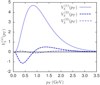
Note that the quantities in this table are proportional to the square-root of the eigenvalues, . From the decreasing magnitudes of the listed (scaled) magnitudes, we see that the first two eigenmodes account for 99.9% of the squared variance, which can be represented as a sum of the eigenvalues
| (18) |
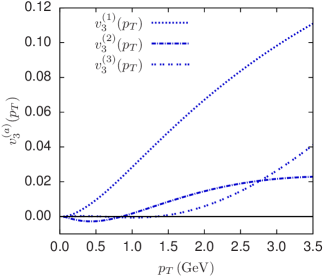
Figure 1(a) displays the eigenvectors, , for the leading and first two subleading modes. We see that only the first two flow modes are significant, and in the rest of this paper we consider only these two. To make contact with the more traditional definitions of , we divide by and present the same eigenmodes in Fig. 1(b).
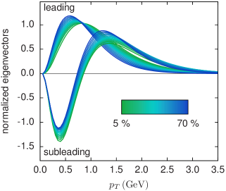
We also investigated the centrality and viscosity dependence of the principal components. The normalized principal flow eigenvectors are approximately independent of viscosity (not shown). In Fig. 2, we show the centrality dependence of these normalized eigenvectors. In more central collisions the eigenvectors shift to larger transverse momentum, which can be understood with the system size scaling introduced in Ref. Başar and Teaney (2014).
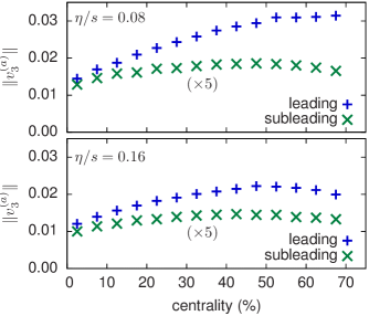
The magnitude of the flow, i.e. the squared integral , depends on both centrality and viscosity. To factor out the trivial multiplicity dependence of , we plot the scaled flow eigenvalues [see Eq. (10)] in Fig. 3. Going from to we see significant suppression of the leading mode. In general the subleading scaled flow depends weakly on centrality.
IV Geometric Predictors for Subleading Flow
IV.1 Average geometry in the subleading plane
In this section, we clarify the physical origin of the subleading flow by correlating the subleading hydrodynamic response with the geometry.
As a first step, we determined the average initial geometry in the principal component plane. Specifically, for each event the phase of the principal component [see Eq. (11)] defines orientation of the flow. We then rotate each event into plane and average the initial entropy density, . More precisely, the event-by-event geometry in the principal component plane is defined to be
| (19) |
where we have averaged over the phases of . Next, we average over all events weighted by the magnitude of the flow
| (20) |
Figure 4 shows the in-plane averaged geometry for the leading and subleading principal components in central collisions.
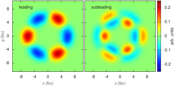
Clearly, the leading principal component is strongly correlated with the triangular components of the initial geometry, while the subleading component is correlated with the radial excitations of this geometry.
To give a one-dimensional projection of Fig. 4, we integrate Eq. (20) over the azimuthal angle to define
| (21) |
This is equivalent to defining ,
| (22) |
and correlating this with the flow fluctuation
| (23) |
Results for are shown by the blue (gray) curves in Fig. 5.
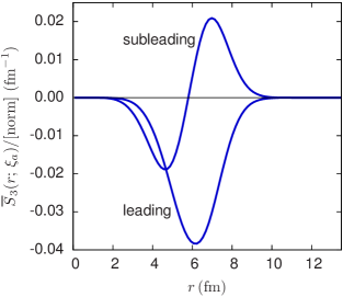
Again we see that the leading flow originates from a geometric fluctuation with a large integrated eccentricity, while the subleading flow is sensitive to the radial excitation of the triangularity. Note that the relatively small subleading flow corresponds to a fairly significant fluctuation of the initial geometry.
IV.2 The average geometry in Fourier space
It is evident from Fig. 5 that the leading and subleading geometries have different characteristic wave numbers. This becomes apparent when we correlate the flow signal with the Fourier (or Hankel) transform of the triangular geometry
| (24) |
Here has the meaning of the th harmonic of the 2D Fourier transform of the initial geometry , i.e. .
We recall that the is determined by the long wavelength limit of Teaney and Yan (2011)
| (25) |
where is the root mean square radius and is the total entropy in a given centrality bin. The constant factors are determined by the expansion of near . Motivated by this limit we define a generalized eccentricity
| (26) |
which approaches as . Clearly in a Glauber model there is an analogous definition
| (27) |
where the coordinates of the th participant are .
The Pearson correlation coefficient between the flow and a specific wave number is
| (28) |
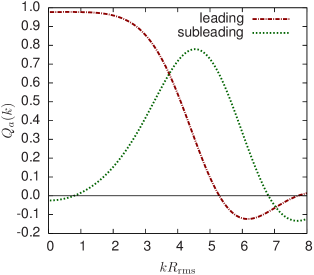
Examining in Fig. 6, we see that leading component is produced by low- fluctuations, while subleading flow originates from fluctuations at larger .
IV.3 Optimal geometric predictors for the subleading flow
In this section, our aim is to predict the magnitude and orientation of the leading and subleading flows. To this end we regress each principal component of the flow with various Fourier components of the initial geometry.
Following Ref. Gardim et al. (2012), we construct a prediction for the flow amplitude by taking a linear combination of :
| (29) |
The selected wave numbers are discussed in the next paragraph. The response coefficients are chosen to minimize the square error , or equivalently to maximize the Pearson correlation coefficient between the flow and the prediction
| (30) | |||
| (31) |
The correlation coefficient is referred to as the quality coefficient in Ref. Gardim et al. (2012).
We construct two predictors based on two and five wave numbers. For the five-term predictor we choose equidistant points which span the range seen in Fig. 6
| (32) |
and fit the response coefficients . The two term predictor was motivated by the discrete Fourier-Bessel series advocated for in Ref. Floerchinger and Wiedemann (2014),
| (33) |
where are the zeros of , and we select to optimize the correlation between the geometrical predictor and the flow. For comparison, we also constructed a two term linear predictor from the familiar eccentricities and defined in Eqs. (3a) and (3b).
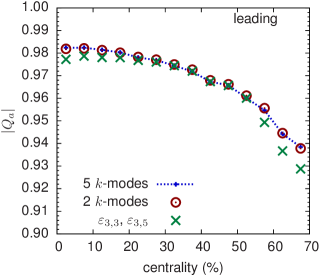
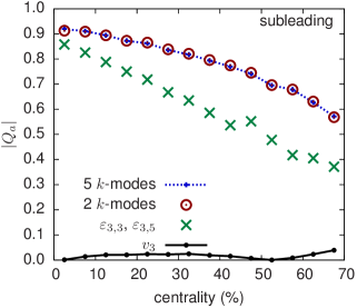
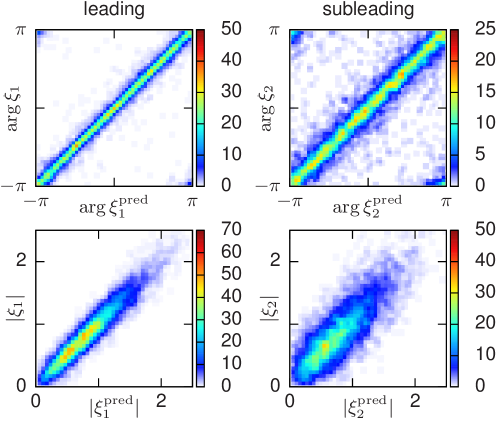
In Figs. 7(a) and (b) we show the correlation coefficient between the leading and subleading flow amplitudes and the predicted amplitudes using the two and five Fourier mode fits, and the , fit. As is well known, the leading mode is very well predicted by and , though the quality degrades towards peripheral collisions. These results for the leading mode can be compared profitably with Fig. 4 of Ref. Gardim et al. (2015), where similar results were recently reported. For the subleading flow the linear correlation coefficient is reduced relative to the leading flow, and a high degree of correlation is only achieved for the 0–40% centrality range. The simple geometric predictor based on and is reasonably correlated with the subleading flow in central collisions, but this correlation rapidly deteriorates in more peripheral collisions. The predictor based on two judiciously chosen wave numbers generally outperforms all other predictors we studied for both the leading and subleading modes. Indeed, we believe based on numerous other fits that these two wave numbers essentially exhaust the predictive power of the event-by-event triangular geometry, . Additional histograms correlating the amplitudes and phases of the flow and the two-term prediction are shown in Fig. 12 in the appendix.
The two-wave-number fit correlates the flow with a specific projection of the triangular geometry, i.e.
| (34) |
where is a radial weight chosen to maximize the correlation between the flow and the projection. This is analogous to using to predict triangular flow, where the radial weight is
| (35) |
We have used Fourier modes as a basis for ,
| (36) |
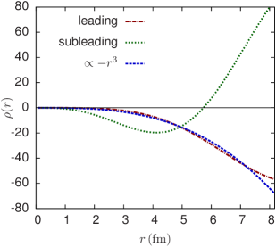
but other functions could have been used.555A table of is given as a function of centrality in the appendix. In Fig. 8 we compare the radial weights for the leading and subleading modes. The overall normalization of weight function is adjusted so that
| (37) |
The weight function for the leading projector is very close to cubic weight, but the subleading radial weight has a node at .
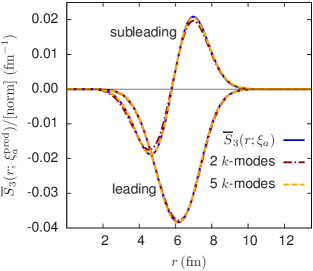
Within the framework of linear response, in Sec. IV.1 we found the optimal geometry for predicting the leading and subleading flows by correlating the observed flow with the geometry, . To test if the two and five wave number predictors reproduce this optimal geometry, we formed the analogous correlator between the predicted flow and , . Examining Fig. 9, we see that the two term predictor fully captures the optimal average geometry. For peripheral collisions the optimal geometry differs from what we can construct using linear combinations of Fourier modes, suggesting that additional nonlinear physics Qiu and Heinz (2011); Gardim et al. (2012); Teaney and Yan (2012) plays a role in determining the subleading flow.
Figure 7(b) also shows the correlation (or lack thereof) between the subleading flow and the integrated
| (38) |
Since the subleading mode is uncorrelated with the leading mode (by construction), there is almost no correlation between the integrated and the subleading mode. The upshot is that measurements of based on the event plane or scalar product method are projecting out the important physics of the subleading mode.
V Testing Linear Response
The success of the linear flow predictors discussed in previous section depends on the applicability of linear response. A straightforward way to check this assumption is to compare the averaged response of event-by-event hydrodynamics to the hydrodynamic response to suitably averaged initial conditions.
In Sec. IV.1 we computed the average geometry in the event planes of the leading and subleading flows (see Fig. 4). It is straightforward to simulate this smooth initial condition and to compute the associated . This is known as “single-shot” hydrodynamics in the literature Qiu and Heinz (2011). In Fig. 10 we compare from the leading and subleading average geometries to the principal components and of event-by-event hydro.
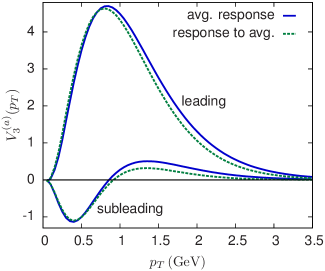
The qualitative features of both principal components are reproduced well by single-shot hydrodynamics, especially for the leading flow. It is particularly notable how the single-shot evolution reproduces the change of sign in . However, in an important range, , the single-shot evolution misses the event-by-event curve for subleading flow by .
It is useful to examine the time development of the subleading flow in the single-shot hydrodynamics. In Fig. 11, we present three snapshots of the subleading flow evolution. The color contours show the radial momentum density per rapidity,
| (39) |
as a function of proper time .
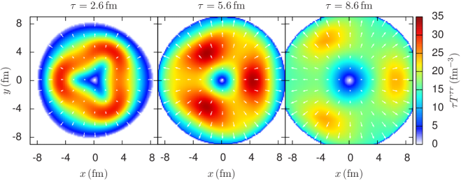
Shortly after the formation of the fireball, at we observe negative triangular flow in Fig. 11(a). This flow is produced by the excess of material at small radii flowing into the “valleys” at larger radii [see Fig. 4(b)]. However, the radial flow has not developed yet, and therefore this phase of the evolution creates negative flow at small transverse momentum. After this stage, we see typical flow evolution of a triangular perturbation, i.e. the negative geometric eccentricity at small radii is transformed into positive triangular flow at large transverse momentum [see Figs. 11(b) and (c)]. The inner eccentricity dominates over the outer eccentricity at high because the radial flow has more time to develop before freeze-out, and because there is more material at small radii.
VI Discussion
This paper illustrates how principal component analysis can be used to understand the physics encoded in the two particle correlation matrix of hydrodynamics. PCA is an economical way to summarize the factorization breaking in these correlations. More precisely, we found that the matrix of correlation coefficients in hydrodynamics, Eq. (1), is completely described by two principal components, and as written in Eq. (2). Importantly, these components have a simple physical interpretation—they are the hydrodynamic response to two statistically independent initial conditions in the fluctuating geometry. The leading principle component is the hydrodynamic response to the participant triangularity, while the subleading flow (which is uncorrelated with the leading flow) is the hydrodynamic response to the first radial excitation of the triangularity. This conclusion was reached by averaging the event-by-event geometry in the event plane of the subleading flow (Fig. 4). The magnitude of this radial excitation is on par with the magnitude of the triangularity (Fig. 5), although the hydro response is smaller in magnitude. Since the subleading component is uncorrelated with the integrated , it is projected out in analyses of triangular flow based on the scalar product or event plane methods.
We first studied the basic properties of the subleading flow such as its dependence on transverse momentum (Fig. 1), and centrality and shear viscosity (Fig. 3). The flow response is approximately linear to the geometrical deformation. This was checked by simulating the response to the average in-plane geometry with “single-shot” hydrodynamics (Fig. 11), and comparing this result to event-by-event hydrodynamics; i.e., we compared the response to the average with the averaged response (Fig. 10).
Motivated by the linearity of the response, we constructed a geometrical predictor for the subleading flow analogous to . We first defined as the Fourier mode of the event-by-event triangular geometry up to normalization.666 The normalization is chosen so that . Then we constructed a linear geometrical predictor for the leading and subleading flow angles and magnitudes based on two Fourier modes (Figs. 7 and 12). Indeed, the subleading flow response is proportional to an event-by-event quantity which captures the radial excitation of the triangular geometry,
| (40) |
where is the initial entropy distribution, and is an appropriate excited radial weight function. The two term Fourier fit to is tabulated in the appendix and graphed in Fig. 8. The subleading flow probes the initial state geometry at higher wave numbers than the leading flow (Fig. 6). We found that the correlation between the flow and the Fourier components of the geometry is maximized for wave numbers away from zero, . Thus, the subleading flow provides a new test of viscous hydrodynamics and initial-state models.
In peripheral collisions the correlation between the linear geometrical
predictor and the flow is smaller. This suggests that nonlinear dynamics at
large impact parameters couples the average elliptic geometry to the harmonic
perturbations Qiu and Heinz (2011); Gardim et al. (2012); Teaney and Yan (2012). The statistical
tools such as PCA and related methods developed in this work can be used to
clarify this complex hydrodynamic response.
Acknowledgments:
We thank J. Y. Ollitrault, E. Shuryak, and J. Jia for continued interest. We
especially thank S. Mohapatra for simulating hydro events. This work was supported by the Department of Energy,
DE-FG-02-08ER41450.
Appendix A Two term predictor
Here we present the best fit results for the two wave number predictor, see eqs. (34), (36) and (37),
| (41) |
Table 2 records the ratios of fit coefficients for the leading and subleading predictors.
| centrality | leading | subleading |
|---|---|---|
| 0-5% | -0.93 | -2.61 |
| 5-10% | -0.87 | -2.89 |
| 10-15% | -0.83 | -3.03 |
| 15-20% | -0.78 | -3.08 |
| 20-25% | -0.73 | -3.16 |
| 25-30% | -0.70 | -3.18 |
| 30-35% | -0.63 | -3.22 |
| 35-40% | -0.58 | -3.17 |
| 40-45% | -0.53 | -3.15 |
| 45-50% | -0.44 | -3.12 |
| 50-55% | -0.35 | -3.07 |
| 55-60% | -0.23 | -3.02 |
| 60-65% | -0.06 | -2.99 |
| 65-70% | 0.08 | -2.88 |
In Fig. 12 we show the correlations between the flow and its predictor for both the angles and magnitudes. The subleading flow direction correlates well with the predictor, and there is reasonable correlation for the magnitude as well.
References
- Heinz and Snellings (2013) Ulrich Heinz and Raimond Snellings, “Collective flow and viscosity in relativistic heavy-ion collisions,” Ann. Rev. Nucl. Part. Sci. 63, 123–151 (2013), arXiv:1301.2826 [nucl-th] .
- Luzum and Petersen (2014) Matthew Luzum and Hannah Petersen, “Initial State Fluctuations and Final State Correlations in Relativistic Heavy-Ion Collisions,” J. Phys. G41, 063102 (2014), arXiv:1312.5503 [nucl-th] .
- Alver and Roland (2010) B. Alver and G. Roland, “Collision geometry fluctuations and triangular flow in heavy-ion collisions,” Phys. Rev. C81, 054905 (2010), [Erratum: Phys. Rev.C82,039903(2010)], arXiv:1003.0194 [nucl-th] .
- Gardim et al. (2013) Fernando G. Gardim, Frederique Grassi, Matthew Luzum, and Jean-Yves Ollitrault, “Breaking of factorization of two-particle correlations in hydrodynamics,” Phys. Rev. C87, 031901 (2013), arXiv:1211.0989 [nucl-th] .
- Heinz et al. (2013) Ulrich Heinz, Zhi Qiu, and Chun Shen, “Fluctuating flow angles and anisotropic flow measurements,” Phys. Rev. C87, 034913 (2013), arXiv:1302.3535 [nucl-th] .
- Kozlov et al. (2014) Igor Kozlov, Matthew Luzum, Gabriel Denicol, Sangyong Jeon, and Charles Gale, “Transverse momentum structure of pair correlations as a signature of collective behavior in small collision systems,” (2014), arXiv:1405.3976 [nucl-th] .
- Bhalerao et al. (2015) Rajeev S. Bhalerao, Jean-Yves Ollitrault, Subrata Pal, and Derek Teaney, “Principal component analysis of event-by-event fluctuations,” Phys. Rev. Lett. 114, 152301 (2015), arXiv:1410.7739 [nucl-th] .
- Teaney and Yan (2011) Derek Teaney and Li Yan, “Triangularity and Dipole Asymmetry in Heavy Ion Collisions,” Phys. Rev. C83, 064904 (2011), arXiv:1010.1876 [nucl-th] .
- Qiu and Heinz (2011) Zhi Qiu and Ulrich W. Heinz, “Event-by-event shape and flow fluctuations of relativistic heavy-ion collision fireballs,” Phys. Rev. C84, 024911 (2011), arXiv:1104.0650 [nucl-th] .
- Baier et al. (2008) Rudolf Baier, Paul Romatschke, Dam Thanh Son, Andrei O. Starinets, and Mikhail A. Stephanov, “Relativistic viscous hydrodynamics, conformal invariance, and holography,” JHEP 04, 100 (2008), arXiv:0712.2451 [hep-th] .
- Dusling and Teaney (2008) K. Dusling and D. Teaney, “Simulating elliptic flow with viscous hydrodynamics,” Phys. Rev. C77, 034905 (2008), arXiv:0710.5932 [nucl-th] .
- Teaney and Yan (2012) Derek Teaney and Li Yan, “Non linearities in the harmonic spectrum of heavy ion collisions with ideal and viscous hydrodynamics,” Phys. Rev. C86, 044908 (2012), arXiv:1206.1905 [nucl-th] .
- Alver et al. (2008) B. Alver, M. Baker, C. Loizides, and P. Steinberg, “The PHOBOS Glauber Monte Carlo,” (2008), arXiv:0805.4411 [nucl-ex] .
- Qiu (2013) Zhi Qiu, Event-by-event Hydrodynamic Simulations for Relativistic Heavy-ion Collisions, Ph.D. thesis, Ohio State U. (2013), arXiv:1308.2182 [nucl-th] .
- Laine and Schroder (2006) Mikko Laine and York Schroder, “Quark mass thresholds in QCD thermodynamics,” Phys. Rev. D73, 085009 (2006), arXiv:hep-ph/0603048 [hep-ph] .
- Luzum and Romatschke (2008) Matthew Luzum and Paul Romatschke, “Conformal Relativistic Viscous Hydrodynamics: Applications to RHIC results at s(NN)**(1/2) = 200-GeV,” Phys. Rev. C78, 034915 (2008), [Erratum: Phys. Rev.C79,039903(2009)], arXiv:0804.4015 [nucl-th] .
- Başar and Teaney (2014) Gökçe Başar and Derek Teaney, “Scaling relation between pA and AA collisions,” Phys. Rev. C90, 054903 (2014), arXiv:1312.6770 [nucl-th] .
- Gardim et al. (2012) Fernando G. Gardim, Frederique Grassi, Matthew Luzum, and Jean-Yves Ollitrault, “Mapping the hydrodynamic response to the initial geometry in heavy-ion collisions,” Phys. Rev. C85, 024908 (2012), arXiv:1111.6538 [nucl-th] .
- Floerchinger and Wiedemann (2014) Stefan Floerchinger and Urs Achim Wiedemann, “Statistics of initial density perturbations in heavy ion collisions and their fluid dynamic response,” JHEP 08, 005 (2014), arXiv:1405.4393 [hep-ph] .
- Gardim et al. (2015) Fernando G. Gardim, Jacquelyn Noronha-Hostler, Matthew Luzum, and Frédérique Grassi, “Effects of viscosity on the mapping of initial to final state in heavy ion collisions,” Phys. Rev. C91, 034902 (2015), arXiv:1411.2574 [nucl-th] .