Numerical implementation of the multiscale and averaging methods for quasi periodic systems

Abstract.

We consider the problem of numerically solving the Schrödinger equation with a potential that is quasi periodic in space and time. We introduce a numerical scheme based on a newly developed multi-time scale and averaging technique. We demonstrate that with this novel method we can solve efficiently and with rigorous control of the error such an equation for long times. A comparison with the standard split-step method shows substantial improvement in computation times, besides the controlled errors. We apply this method for a free particle driven by quasi-periodic potential with many frequencies. The new method makes it possible to evolve the Schrödinger equation for times much longer than was possible so far and to conclude that there are regimes where the energy growth stops in-spite of the driving.

1. Introduction

A method for the study of the dynamics for the Schrödinger equation with time dependent potentials [1] is implemented numerically. The potential is quasiperiodic in both space and time. The power of this new method is demonstrated. Exploration of the dynamics for such potentials is motivated by experiments in optics [2] where hypertransport, namely transport faster then ballistic was found experimentally and numerically in some regimes. In theoretical work that followed [2, 3, 4, 5] a classical theory was developed for the potentials relevant for these optics experiments. In particular, it was found in the framework of classical mechanics, that for smooth potentials the spreading in momentum as function of time stops. The calculations of the present paper are for such potentials. For short times, relevant for the existing experiments it was found that wave or quantum and classical dynamics agree in general features.
For long times it turned out impossible to compute numerically the quantum dynamics using the standard methods [6, 7], while with the method introduced in [1] and implemented here, calculations for such long times are feasible as will be demonstrated in this paper. Such calculations and comparison with the classical results, is of fundamental importance for the issue of quantum classical correspondence. The main objective of the present paper is to demonstrate the power of the method introduced in [1] for a physically relevant example.

Potentials which are quasiperodic both in space and time, can manifest a high degree of complexity and are subject of many studies over the last decade, mostly in the framework of classical physics [8, 9, 10, 11, 12, 13, 14]. With different experimental realizations of such potentials there is also a need for a numerical approach to investigate them and their asymptotic behavior. The standard way to numerically solve problems with time dependent potentials is based on either spectral methods [15, 16] or explicit/implicit finite difference schemes [7, 17]. In this paper we implement numerically a recently developed rigorously controlled multi-time scale averaging technique [1]. The above mentioned method has two distinct advantages. The first is that at each step of the averaging hierarchy there is a well defined and completely known bound on the numerical error. The second advantage and one which has far greater impact is the reduction in computational time accompanied with each of the hierarchical averaging steps. This reduction enables us to go to long time scales, impossible by the methods we are aware of. In this paper we describe and present an implementation for a specific problem.

The outline of the paper is as follows. In Section 2, we present the model for which the method of multiple scale and averaging (MSA) is implemented. This model is of physical interest and importance. The MSA method that was developed in Ref. [1] and details of its implementation are presented in Secs. 3 and 4. The MSA method involves a hierarchy of computations where the first level is described is Sec. 3 and the following levels are presented in Section 4. The needed level is determined by the required precision and the time over which the system is evolved. In Section 5 we demonstrate that the MSA method is superior compared to the standard split step method, since for the same precision it is much faster. Moreover for the split step method there is only an empirical estimate on the error while for the MSA there is a rigorous bound. Using it in Section 6, we show that with the help of this method we could solve the Schrödinger equation for the model problem presented in Section 2, for an extremely long time; we conclude that for this model the energy does not grow to infinity in-spite of the time dependent driving potential. The spreading in the quantum case is wider than in the corresponding classical system. This results from the fact that initially we observe a lot of spreading in the quantum case, while the classical case does not show spreading.

2. The model that will be studied

In this section we introduce the model for which our MSA method developed in [1] is implemented. In the first subsection its relation to physical systems is explained, while in the second one it is reduced to a form for which the MSA method can be applied(see Eqs. 2.11-2.13).

2.1. The physical model

The random potentials which are prepared in optics [18, 2] and atom optics [19, 20, 21] experiments, are described by a sum of random Fourier components. In experiments, potentials which are composed out of a large number of random independent Fourier components $N$, are created .
More specifically here, the Schrödinger equation for a potential

(2.1) $$V\left(x^{\prime},\tau\right)=\frac{1}{\sqrt{N}}\sum_{n=1}^{N}A_{n}\exp\left(i(k_{n}x^{\prime}-\omega^{\prime}_{n}\tau)\right)+\mathcal{C}.\mathcal{C}$$

is used. The $A_{m}$ are independent, identically distributed complex random variables, where $\mathcal{C}.\mathcal{C}$ stands for complex conjugate. The expectation values of these variables satisfy

(2.2) $$<A_{m}>=<A_{m}A_{n}>=0\ \ \ <A_{m}{A_{n}}^{*}>=\sigma^{2}\delta_{nm}$$

We will study the specific model where $A_{n}=A\ e^{i\phi_{m}}$ with $\phi_{m}$ uniformly distributed in the interval $[-\pi,\pi]$ and $A>0$. The distribution of $\omega_{n}$ and $k_{n}$ is specified in Section 5.
The equation of motion is the time dependent Schrödinger equation

(2.3) $$i\partial_{\tau}\psi\left(x^{\prime},\tau\right)=H\psi\left(x^{\prime},\tau\right).$$

Where

(2.4) $$H=\frac{1}{2}p^{\prime 2}+V(x^{\prime},\tau),$$

$$p^{\prime}=-i\nabla_{x^{\prime}}.$$

In the following section we will introduce the reduction of the problem to a form where the MSA technique is applicable.

2.2. Reduction of the problem

In the model with potential given by (2.1), the particle is expected to be accelerated most effectively in the regime of velocities where the Chirikov resonances

(2.5) $$v_{n}^{(r)}=\frac{\omega^{\prime}_{n}}{k_{n}}$$

are formed [22, 23].
In this paper we choose $v_{n}^{(r)}$ and $k_{n}$ uniformly distributed in the intervals $\left[v^{\left(\text{min}\right)},v^{\left(\text{max}\right)}\right]$ and $\left[k^{\left(\text{min}\right)},k^{\left(\text{max}\right)}\right]$ respectively. The crucial point is that the Chirikov resonant velocities are bounded in a phase space strip. This is typically the case for smooth potentials, and will be assumed in this paper.
Here we would like to study what is the acceleration of a particle prepared with momentum or velocity $v$ (we assume unit mass), so that all $v_{n}^{(r)}$ are far from $v$. For the classical corresponding system we found that the acceleration is negligible [3, 5, 4]. Here we study the corresponding quantum mechanical system. For this purpose it is convenient to work in a frame of reference where the initial velocity of the particle vanishes. For this we perform the Galilean transformation

(2.6) $$x=x^{\prime}-v\tau,$$

where $v$ is the velocity of the moving frame (in later stages we will relate this quantity to the required small parameter) on the potential (2.1)

(2.7) $$V\left(x+v\tau,\tau\right)=\frac{A}{\sqrt{N}}\sum_{n=1}^{N}\cos\left(k_{n}\left(x+v\tau\right)-\omega^{\prime}_{n}\tau+\phi_{n}\right)$$

$$=\frac{A}{\sqrt{N}}\sum_{n=1}^{N}\cos\left(k_{n}x+\left(k_{n}v-\omega^{\prime}_{n}\right)\tau+\phi_{n}\right).$$

Now, re-scaling time as

(2.8) $$t=\tau v,$$

the potential takes the form

(2.9) $$V\left(x,t\right)=\frac{A}{\sqrt{N}}\sum_{n=1}^{N}\cos\left(k_{n}x-\frac{\left(\omega^{\prime}_{n}-k_{n}v\right)}{v}t+\phi_{n}\right)$$

and defining

(2.10) $$\omega{}_{n}=\frac{\left(\omega^{\prime}_{n}-k_{n}v\right)}{v}$$

The potential in the moving frame takes the form

(2.11) $$V\left(x,t\right)=\frac{A}{\sqrt{N}}\sum_{n=1}^{N}\cos\left(k_{n}x-\omega{}_{n}t+\phi_{n}\right)$$

The time dependent Schrödinger equation is

(2.12) $$i\partial_{t}\psi\left(x,t\right)=\frac{1}{v}H(p,x,t)\psi\left(x,t\right)$$

Introducing the small parameter $\beta=\frac{1}{v}$:

(2.13) $$i\partial_{t}\psi\left(x,t\right)=\beta H(p,x,t)\psi\left(x,t\right)$$

From this point on we will use the small parameter $\beta$ to perform the averaging steps introduced in the next section. In what follows we will also relate the small parameter $\beta$ to the time scale on which we average. The Hamiltonian will be approximated by a finite matrix (in space and momentum) and it will be verified that the spreading never reaches the boundaries set by this basis.

3. The averaging scheme

The multiscale averaging method is based on replacing the original Hamiltonian by a hierarchical set of averaged Hamiltonians. In each step we perform a “peel-off” transformation and average a part of the Hamiltonian, for a chosen time interval of length $T_{0}=\frac{1}{\sqrt{\beta}}=\sqrt{v}$.  This choice is not unique, but as shown in [1] leads to effective error bounds. We use the fact that Eq (2.13) is of the form of (2.1) in [1].

In this section the implementation of the MSA method of [1] for equation (2.13) will be presented. In Appendix A we summarize the main results of Ref. [1]

3.1. Zero order

The zero order average on the jth time interval has the form ($V\left(t\right)\equiv V\left(x,t\right)$)

(3.1) $$\bar{V}_{0}^{\left(j\right)}=\frac{1}{T_{0}}\int_{jT_{0}}^{(j+1)T_{0}}V\left(t\right)dt$$

In the case of the potential (2.1), the zero order averaging can be performed analytically

(3.2) $$\bar{V}_{0}^{\left(j\right)} = \frac{1}{T_{0}}\int_{jT_{0}}^{(j+1)T_{0}}V\left(t\right)dt=\frac{A}{\sqrt{N}T_{0}}\int_{jT_{0}}^{(j+1)T_{0}}\sum_{n=1}^{N}\cos\left(k_{n}x-\omega{}_{n}t+\phi_{n}\right)=$$

$$= \frac{A}{\sqrt{N}T_{0}}\sum_{n=1}^{N}\frac{1}{\omega}\left[\sin\left(k_{n}x-\omega{}_{n}\left(j+1\right)T_{0}+\phi_{n}\right)\right.$$

$$\left.-\sin\left(k_{n}x-\omega{}_{n}jT_{0}+\phi_{n}\right)\right]=$$

$$= 2\frac{A}{\sqrt{N}T_{0}}\sum_{n=1}^{N}\frac{1}{\omega_{n}}\sin\left(\frac{1}{2}\omega{}_{n}T_{0}\right)\cos\left(k_{n}x-\omega{}_{n}\left(j+\frac{1}{2}\right)T_{0}+\phi_{n}\right)$$

This defines the Hamiltonian on one time interval; accordingly we can write the Hamiltonian of one interval as

(3.3) $$\bar{H}_{0}^{(j)}\left(x\right)=-\frac{1}{2}\frac{\partial^{2}}{\partial x^{2}}+\bar{V}_{0}^{\left(j\right)}\left(x\right)$$

The global Hamiltonian corresponding to (2.1) of [1], which gives the zeroth order approximation to $H\left(t\right)$, is generated by:

(3.4) $$\bar{H}_{0}^{g}={\bar{H}_{0}}^{(j)}(t)\ \ \text{for}\ \ jT_{0}\leq t<(j+1)T_{0}.$$

Using this notation, a general time evolution can be written as the product of the interval propagators since $\bar{H}_{0}^{g}$ is piecewise constant in time,

(3.5) $$U_{0}\left(t\right)=e^{-i\beta\bar{H}_{0}^{(j_{max})}\left(t-j_{max}T_{0}\right)}\dots e^{-i\beta\bar{H}_{0}^{(1)}T_{0}}e^{-i\beta\bar{H}_{0}^{(0)}T_{0}}$$

where $j_{max}-1$ is the integer part of $t/T_{0}$ The evolution in this order is

(3.6) $$\psi_{0}\left(x,t\right)=U_{0}\left(t\right)\psi\left(x,0\right).$$

The propagator satisfies

(3.7) $$i\frac{\partial}{\partial t}U_{0}(t)=\beta\bar{H}_{0}^{(g)}U_{0}(t)$$

corresponding to (2.10) of [1]. This propagator is numerically implemented and used to solve the time dependent equation of motion. The error in this order is bounded by $\beta^{\frac{1}{2}}$ up to times of order $T_{0}$, the reasoning behind this is shown in [1], Eq. (2.49) there. The error in diagonalization of $\bar{H}_{0}^{\left(j\right)}$ is negligible (see discussion in Sec. 5)

3.2. First order

The first order averaging is based upon a “peel-off” transformation of the zero order. In such a transformation the next order Hamiltonian is constructed from the zero order in the following way: Let $H_{1}\left(t\right)$ be defined as

(3.8) $$H_{1}\left(t\right)=U_{0}^{-1}\left(t\right)\left[H\left(t\right)-\bar{H_{0}}^{g}\left(t\right)\right]U_{0}\left(t\right)$$

Hence $H_{1}\left(t\right)$ is the Heisenberg dynamics of the full problem with $U_{0}\left(t\right)$ dynamics peeled off. An important point to note is that the Laplacian term drops in $H_{1}!$ Hence $H_{1}\left(t\right)$ is a bounded operator, for which the results of [1] directly apply. Its average in the j-th interval is

(3.9) $$\bar{H}_{1}^{\left(j\right)}=\frac{1}{T_{0}}\int_{jT_{0}}^{\left(j+1\right)}H_{1}\left(t\right)dt$$

The $\bar{H}_{1}\left(t\right)$ dynamics is given by the propagator

(3.10) $$U_{1}\left(t\right)=e^{-i\beta\bar{H}_{1}^{(j_{max})}\left(t-j_{max}T_{0}\right)}\dots e^{-i\beta\bar{H}_{1}^{(0)}T_{0}}$$

We turn now to calculate $\bar{H}_{1}^{\left(j\right)}$, by (2.49) of [1] it is of order $\sqrt{\beta}$. Before diagonalizing this operator in order to calculate the time evolution, there are several steps needed to be taken. First we write explicitly $\bar{H_{1}}^{\left(j\right)}$ using integration by parts

(3.11) $$\bar{H_{1}}^{\left(j\right)}=\frac{1}{T_{0}}\int_{jT_{0}}^{(j+1)T_{0}}U_{0}^{-1}(t)\left[H\left(t\right)-\bar{H}_{0}^{g}\left(t\right)\right]U_{0}(t)dt=\bar{H_{1}}^{\left(j,\text{I}\right)}+\bar{H_{1}}^{\left(j,\text{II}\right)}+\bar{H_{1}}^{\left(j,\text{III}\right)},$$

where

(3.12) $$\bar{H_{1}}^{\left(j,\text{I}\right)}=\frac{1}{T_{0}}\left[U_{0}^{-1}(t)\left(\int_{0}^{t}\left[H\left(t^{\prime}\right)-\bar{H}_{0}^{g}\left(t^{\prime}\right)\right]dt^{\prime}\right)U_{0}(t)\right]\begin{array}[]{c}(j+1)T_{0}\\ t=jT_{0}\end{array}$$

(3.13) $$\bar{H_{1}}^{\left(j,\text{II}\right)}=-\frac{1}{T_{0}}\int_{nT_{0}}^{(n+1)T_{0}}dt^{\prime}\left(\frac{\partial}{\partial t^{\prime}}U_{0}^{-1}(t^{\prime})\right)\left[\int_{0}^{t^{\prime}}\left[H\left(s\right)-\bar{H}_{0}^{g}\left(s\right)\right]ds\right]U_{0}(t^{\prime}),$$

and

(3.14) $$\bar{H_{1}}^{\left(j,\text{III}\right)}=-\frac{1}{T_{0}}\int_{jT_{0}}^{(j+1)T_{0}}U_{0}^{-1}(t^{\prime})\left[\int_{0}^{t^{\prime}}\left[H\left(s\right)-\bar{H}_{0}^{g}\left(s\right)\right]ds\right]\left(\frac{\partial}{\partial t}U_{0}\right)(t^{\prime})dt^{\prime}.$$

We note that for any integer $t/T_{0}$,

(3.15) $$\int_{jT_{0}}^{\left(j+1\right)T_{0}}\left[H\left(t^{\prime}\right)-\bar{H}_{0}^{g}\left(t^{\prime}\right)\right]dt^{\prime}=0$$

by construction. Therefore for such $t$ $\bar{H_{1}}^{\left(j,\text{I}\right)}\left(t\right)=0$ and $\bar{H_{1}}^{\left(j,\text{II}\right)}\left(t\right)$ can be simplified. Moreover the expression in $\bar{H_{1}}^{\left(j,\text{III}\right)}$ is just the hermitian conjugate of $\bar{H_{1}}^{\left(j,\text{II}\right)}$ so we only need to analyze the second term:

$$\bar{H_{1}}^{\left(j,\text{II}\right)} = \frac{1}{T_{0}}\int_{jT_{0}}^{(j+1)T_{0}}dt^{\prime}\left(\frac{\partial}{\partial t^{\prime}}U_{0}^{-1}(t^{\prime})\right)\left[\int_{jT_{0}}^{t^{\prime}}\left[H_{j}\left(s\right)-\bar{H_{0}}^{\left(g\right)}\left(s\right)\right]ds\right]U_{0}(t^{\prime})$$

$$=\frac{1}{T_{0}}\int_{jT_{0}}^{(j+1)T_{0}}dt^{\prime}\left(\frac{\partial}{\partial t^{\prime}}U_{0}^{-1}(t^{\prime})\right)\left[\int_{jT_{0}}^{t^{\prime}}H_{0}\left(s\right)ds-\left(t^{\prime}-jT_{0}\right)\bar{H_{0}}^{\left(j\right)}\right]U_{0}(t^{\prime})$$

To evaluate this operator we can use a recursive construction of states based on the zeroth order eigenstates of the averaged Hamiltonian. It is important to remember that this is actually a matrix. For convenience of notation we will define

(3.17) $$U_{0}\left(t\right)=e^{-i\beta\bar{H}_{0}^{(j)}\left(t-jT_{0}\right)}......e^{-i\beta\bar{H}_{0}^{\left(1\right)}T_{0}}e^{-i\beta\bar{H}_{0}^{\left(0\right)}T_{0}},$$

For $t$ that is an integer multiple of $T_{0}$.

(3.18) $$U_{0}\left(t\right)=\prod_{j^{\prime}=0}^{j}W_{j-j^{\prime}}$$

where

(3.19) $$W_{j}(t)=e^{-i\beta\bar{H}_{0}^{\left(j\right)}T_{0}}.$$

First we assume $t/T_{0}$ is integer and then generalize for any arbitrary $t$. The eigenvalues and eigenfunctions of $\bar{H}_{0}^{\left(j\right)}$ are

(3.20) $$\bar{H}_{0}^{\left(j\right)}\ket{\varphi_{j}^{k}}=E_{j}^{k}\ket{\varphi_{j}^{k}}$$

Here we use a base of size $M$ that is assumed to be finite (in this work we take $M=64$). Since $\beta$ is small the eigenfunctions are approximately eigenfunctions of a free particle, namely

(3.21) $$<x|\varphi_{j}^{k}>\approx e^{i\tilde{k}x}.$$

We will have $M$ eigenvalues and eigenvectors, the largest value of $\left|\tilde{k}\right|$ is 50. Between each pair of propagators $W_{j},W_{i-1}$ we can insert the identity resolution in the corresponding basis (3.20)

(3.22) $$\hat{I}_{j}=\sum_{k=1}^{M}\ket{\varphi_{j}^{k}}\bra{\varphi_{j}^{k}}$$

resulting in

(3.23) $$U_{0}(t)=W_{j}\cdots W_{1}W_{0}=W_{j}\hat{I_{j}}\cdots W_{1}I_{1}W_{0}I_{0}$$

As an example let us take just the first two terms

(3.24) $$W_{1}I_{1}W_{0}I_{0}=\sum_{k_{1}=1}^{M}W_{1}\ket{\varphi_{1}^{k_{1}}}\bra{\varphi_{1}^{k_{1}}}\sum_{k_{0}=1}^{M}W_{0}\ket{\varphi_{0}^{k_{0}}}\bra{\varphi_{0}^{k_{0}}}$$

the brakets expressions $\bra{\varphi_{1}^{k_{1}}}\sum_{k_{0}=1}^{M}W_{0}\ket{\varphi_{0}^{k_{0}}}$ are just scalars, and since $\varphi_{j}^{k_{j}}$ are eigenfunctions of $H_{0}^{j}$ (3.20)

$$W_{1}I_{1}W_{0}I_{0} = \sum_{k_{1}=1}^{M}W_{1}\ket{\varphi_{1}^{k_{1}}}\bra{\varphi_{1}^{k_{1}}}W_{0}\sum_{k_{0}=1}^{M}\ket{\varphi_{0}^{k_{0}}}\bra{\varphi_{0}^{k_{0}}}$$

$$= \sum_{k_{1}=1}^{M}e^{-i\beta T_{0}E_{1}^{k_{1}}}\ket{\varphi_{1}^{k_{1}}}\bra{\varphi_{1}^{k_{1}}}\sum_{k_{0}=1}^{M}e^{-i\beta T_{0}E_{0}^{k_{0}}}\ket{\varphi_{0}^{k_{0}}}\bra{\varphi_{0}^{k_{0}}}$$

using the notation

(3.26) $$\alpha_{k_{1}k_{0}}=\braket{\varphi_{1}^{k_{1}}}{\varphi_{0}^{k{}_{0}}}$$

this becomes

(3.27) $$W_{1}\hat{I}_{1}W_{0}\hat{I}_{0}=\sum_{k_{0}=1}^{M}\sum_{k_{1}=1}^{M}\alpha_{k_{1}k_{0}}e^{-i\beta T_{0}E_{1}^{k_{1}}}e^{-i\beta T_{0}E_{0}^{k_{0}}}\ket{\varphi_{1}^{k_{1}}}\bra{\varphi_{0}^{k_{0}}}$$

In the same way for the complete sequence of propagators (3.18)

$$U_{0}\left(t\right)= \sum_{k_{0}=1}^{M}\dots\sum_{k_{j}=1}^{M}\alpha_{k_{j}k_{j-1}}\alpha_{k_{j-1}k_{j-2}}\dots$$

$$\dots\alpha_{k_{1}k_{0}}e^{-i\beta\left(t-jT_{0}\right)E_{j}^{k_{j}}}\dots e^{-i\beta T_{0}E_{1}^{k_{1}}}e^{-i\beta T_{0}E_{0}^{k_{0}}}\ket{\varphi_{j}^{k_{j}}}\bra{\varphi_{0}^{k_{0}}}.$$

and it satisfies (3.7).
Here $jT_{0}<t<\left(j+1\right)T_{0}$.

The inverse takes the form

$$U_{0}^{-1}(t) = e^{i\beta\bar{H}_{0}^{\left(0\right)}T_{0}}e^{i\beta\bar{H}_{0}^{\left(1\right)}T_{0}}......e^{i\beta\bar{H}_{0}\left(t-jT_{0}\right)}$$

$$= \sum_{k_{j}=1}^{M}\dots\sum_{k_{j-1}=1}^{M}\alpha_{k_{0}k_{1}}^{*}\alpha_{k_{1}k_{2}}^{*}e^{i\beta\left(t-jT_{0}\right)E_{0}}e^{i\beta\left(j-1\right)E_{0}}\ket{\varphi_{0}^{k_{0}}}\bra{\varphi_{j}^{k_{j}}}$$

By (3.7) or direct differentiation of (LABEL:zero_order_prop)

$$\frac{\partial}{\partial t}U_{0}(t) = -\sum_{k_{0}^{{}^{\prime}}=1}^{M}\dots\sum_{k^{\prime}_{j}=1}^{M}\sum_{k_{0}=1}^{M}\dots\sum_{k_{j}=1}^{M}i\beta E_{j}^{k_{j}}\alpha_{k_{j}k_{j-1}}\alpha_{k_{j-1}k_{j-2}}\dots\alpha_{k_{1}k_{0}}$$

$$e^{-i\beta\left(t-jT_{0}\right)E_{j}^{k_{j}}}\dots e^{-i\beta T_{0}E_{0}^{k_{0}}}\ket{\varphi_{j}^{k_{j}}}\bra{\varphi_{0}^{k_{0}}}$$

and in a similar way one finds

(3.31) $$\frac{\partial}{\partial t}U_{0}^{-1}(t)=\sum_{k_{j}=1}^{M}\dots\sum_{k_{j-1}=1}^{M}\alpha_{k_{0}k_{1}}^{*}\alpha_{k_{1}k_{2}}^{*}\dots\alpha_{k_{j-1}k_{j}}^{*}e^{i\beta T_{0}E_{0}^{k_{0}}}\dots e^{i\beta\left(t-jT_{0}\right)E_{j}^{k_{j}}}i\beta E_{j}^{k_{j}}\ket{\varphi_{0}^{k_{0}}}\bra{\varphi_{j}^{k_{j}}}$$

substitution of (3.2) and (LABEL:zero_order_prop) into (3.2) leads to

(3.32) $$\bar{H_{1}}^{\left(j,\text{II}\right)}\left(t\right) = -\frac{1}{T_{0}}\sum_{k_{0}^{{}^{\prime}}=1}^{M}\dots\sum_{k^{\prime}_{j}=1}^{M}\sum_{k_{0}=1}^{M}\dots\sum_{k_{j}=1}^{M}\beta E_{j}^{k_{j}}\alpha_{k^{\prime}_{0}k^{\prime}_{1}}^{*}\dots\alpha_{k^{\prime}_{j-1}k^{\prime}_{j}}^{*}\alpha_{k{}_{j}k{}_{j-1}}\dots\alpha_{k_{1}k_{0}}$$

$$\int_{jT_{0}}^{(j+1)T_{0}}dt^{\prime}e^{i\beta T_{0}E_{0}^{k^{\prime}_{0}}}e^{-i\beta T_{0}E_{0}^{k^{\prime}_{0}}}\dots e^{i\beta\left(t-jT_{0}\right)E_{j}^{k^{\prime}_{j}}}e^{-i\beta\left(t^{\prime}-jT_{0}\right)E_{j}^{k^{\prime}_{j}}}$$

$$\ket{\varphi_{0}^{k_{0}^{\prime}}}\bra{\varphi_{j}^{k_{j}^{\prime}}}\left[\int_{jT_{0}}^{t^{\prime}}H\left(s\right)ds-\left(t^{\prime}-jT_{0}\right)\bar{H_{0}}^{\left(j\right)}\right]\ket{\varphi_{j}^{k_{j}}}\bra{\varphi_{0}^{k_{0}}}=$$

$$= -\frac{1}{T_{0}}\sum_{k_{0}^{{}^{\prime}}=1}^{M}\dots\sum_{k^{\prime}_{j}=1}^{M}\sum_{k_{0}=1}^{M}\dots\sum_{k_{j}=1}^{M}\beta E_{j}^{k_{j}}\alpha_{k^{\prime}_{0}k^{\prime}_{1}}^{*}\dots\alpha_{k^{\prime}_{j-1}k^{\prime}_{j}}^{*}\alpha_{k{}_{j}k{}_{j-1}}\dots\alpha_{k_{1}k_{0}}$$

$$\int_{jT_{0}}^{(j+1)T_{0}}dt^{\prime}e^{-i\beta T_{0}E_{0}^{k^{\prime}_{0}}}\dots e^{i\beta\left(t-jT_{0}\right)E_{j}^{k^{\prime}_{j}}}e^{-i\beta\left(t-jT_{0}\right)E_{j}^{k^{\prime}_{j}}}$$

$$\left\langle\left.\varphi_{j}^{k_{j}}\right|\int_{jT_{0}}^{t^{\prime}}H\left(s\right)ds-\left(t-jT_{0}\right)\bar{H_{0}}^{\left(j\right)}\left|\varphi_{j}^{k^{\prime}_{j}}\right.\right\rangle\ket{\varphi_{0}^{k^{\prime}_{0}}}\bra{\varphi_{0}^{k_{0}}}$$

Finally the full expression for the first order averaged Hamiltonian is, where (3.11) and (3.15) were used,

(3.33) $$\bar{H_{1}}^{\left(j\right)}\left(t\right)=\bar{H_{1}}^{\left(j,\text{II}\right)}\left(t\right)+\left(\bar{H_{1}}^{\left(j,\text{II}\right)}\left(t\right)\right)^{\dagger}.$$

$$\bar{H_{1}}^{\left(j\right)}\left(t\right) = 2\Re\left\{-\frac{1}{T_{0}}\sum_{k_{0}^{{}^{\prime}}=1}^{M}\dots\sum_{k^{\prime}_{j}=1}^{M}\sum_{k_{0}=1}^{M}\dots\sum_{k_{j}=1}^{M}\beta E_{j}^{k_{j}}\alpha_{k^{\prime}_{0}k^{\prime}_{1}}^{*}\dots\alpha_{k^{\prime}_{j-1}k^{\prime}_{j}}^{*}\right.$$

$$\alpha_{k{}_{j}k{}_{j-1}}\dots\alpha_{k_{1}k_{0}}\int_{jT_{0}}^{(j+1)T_{0}}dt^{\prime}e^{-i\beta T_{0}E_{0}^{k^{\prime}_{0}}}\dots e^{i\beta\left(t-jT_{0}\right)E_{j}^{k^{\prime}_{j}}}e^{-i\beta\left(t-jT_{0}\right)E_{j}^{k^{\prime}_{j}}}$$

$$\left.\left\langle\left.\varphi_{j}^{k_{j}}\right|\int_{jT_{0}}^{t^{\prime}}dsH\left(s\right)-\left(t-jT_{0}\right)\bar{H_{0}}^{\left(j\right)}\left|\varphi_{j}^{k^{\prime}_{j}}\right.\right\rangle\right\}\ket{\varphi_{0}^{k^{\prime}_{0}}}\bra{\varphi_{0}^{k{}_{0}}}$$

The integral (3.2) is performed numerically as follows. The domain of integration is derived into squares of size $\Delta t\times\Delta t$. The integral is approximated by a sum of the values of the integrand of the middle points of the squares, multiplied by $\Delta t^{2}$. The error in each term is of the order of $\Delta t^{2}$. This can be improved substantially. Here it is not required since we can obtain the required precision in this simple way.

At first sight this expression (3.2) might seem very complicated but can be understood quite easily; in fact what we have here is a matrix constructed from the sum of matrix products; the terms of the matrix involve only the products of eigenvalues and eigenvectors of $\bar{H}_{0}^{\left(j\right)}$. The benefit of calculating the propagator in this manner is that one only needs to diagonalize the Hamiltonian in each interval only once. As a result of (3.2) the averaged potential is of order $\sqrt{\beta}$ and $\alpha_{k_{j},k_{i}}$ are elements of matrices that are almost diagonal as will be verified aposteriori in Sec. 5. Consequently the error in the calculation of (3.2) is of the order

(3.35) $$\delta I_{t}=\Delta t^{2}$$

By the general theory see (2.15) of [1] the first order propagator takes the form (3.5) with $\bar{H}_{0}^{\left(j\right)}$ replaced by $H_{1}^{\left(j\right)}$ namely with

$$U_{1}=e^{-i\beta\bar{H}_{1}^{(j)}\left(t-jT_{0}\right)}......e^{-i\beta\bar{H}_{1}^{\left(1\right)}T_{0}}e^{-i\beta\bar{H}_{1}^{\left(0\right)}T_{0}}$$

3.3. Normal form transformation

To improve the accuracy we implement the normal form transformation; we will use the form given in Eq. (3.10) of [1]. In our notation this becomes

(3.36) $$\tilde{U}_{1}\left(t\right)=1+i\beta U_{1}^{-1}\left(t\right)\left(\int_{0}^{t}dt^{\prime}\left[H_{1}\left(t^{\prime}\right)-\bar{H}_{1}^{\left(g\right)}\left(t^{\prime}\right)\right]\right)U_{1}\left(t\right).$$

The manner in which we will simplify the above expression will be similar to the method used to calculate $U_{1}$ and $H_{1}$ given in Eq (3.10) and (20), splitting into intervals of length $T_{0}$ and using (3.15), replacing $H_{0}$ by $H_{1}$:

$$\tilde{U}_{1}\left(t\right) = 1+i\beta U_{1}^{-1}\left(\sum_{j^{\prime}=0}^{j}\int_{j^{\prime}T_{0}}^{\left(j^{\prime}+1\right)T_{0}}dt^{\prime}\left[H_{1}\left(t^{\prime}\right)-\bar{H}_{1}^{\left(j^{\prime}\right)}\right]\right.$$

$$\left.+\int_{jT_{0}}^{t}\left[H_{1}\left(t^{\prime}\right)+\bar{H}_{1}^{\left(j\right)}\left(t^{\prime}\right)\right]dt^{\prime}\right)U_{1}\left(t\right).$$

by definition of $\bar{H}_{1}^{\left(j\right)}$

$$\int_{j^{\prime}T_{0}}^{\left(j^{\prime}+1\right)T_{0}}dt^{\prime}\left[H_{1}\left(t^{\prime}\right)-\bar{H}_{1}^{\left(j^{\prime}\right)}\right]=0$$

$$\tilde{U}_{1}\left(t\right) = 1+i\beta U_{1}^{-1}\int_{jT_{0}}^{t}dt^{\prime}\left[H_{1}\left(t^{\prime}\right)-\bar{H}_{1}^{\left(j\right)}\left(t^{\prime}\right)\right]U_{1}\left(t\right)=$$

$$1+i\beta U_{1}^{-1}\left[\left(\int_{jT_{0}}^{t}H_{1}\left(t^{\prime}\right)dt^{\prime}\right)-\left(t-jT_{0}\right)\bar{H}_{1}^{\left(j\right)}\right]U_{1}\left(t\right)$$

and explicitly

(3.39) $$\tilde{U}\left(t\right)=1+i\beta e^{i\beta\bar{H}_{1}^{\left(0\right)}T_{0}}\dots e^{i\beta\bar{H}_{1}^{\left(j\right)}\left(t-jT_{0}\right)}\left[\left(\int_{jT_{0}}^{t}H_{1}\left(t^{\prime}\right)dt^{\prime}\right)-\left(t-jT_{0}\right)\bar{H}_{1}^{\left(j\right)}\right]U_{1}\left(t\right)$$

$$\tilde{U}\left(t\right)=e^{-i\beta\bar{H}_{1}^{\left(j\right)}\left(t-jT_{0}\right)}\dots e^{-i\beta\bar{H}_{1}^{\left(0\right)}T_{0}}.$$

If also the normal form transformation is performed the error is of order $\beta^{\frac{3}{2}}$ .

4. Iterative application and error analysis

To reduce the error we introduce an iterative process. After the normal form transformation is performed we introduce a new Hamiltonian

(4.1) $$\tilde{H}_{1}=\frac{1}{\sqrt{\beta}}\tilde{U}_{1}^{-1}\left[H_{1}-H_{1}^{\left(g\right)}\right]\tilde{U}_{1}$$

where

(4.2) $$\tilde{U}_{1}=U_{0}U_{1}\tilde{U}$$

The wave function at the new level satisfies a Schrödinger equation like (3.12) of [1] with $H_{1}$ playing the role of $\tilde{A}\left(t\right)$ there, and $\beta$ is replaced by $\beta^{3/2}$. Now one starts from an equation like (2.13) with $\beta$ replaced by $\beta^{3/2}$ and $H$ by $\tilde{H}_{1}$. At each step the effective value of $\beta$ is reduced $\left(\beta\rightarrow\beta^{3/2}\right)$, and so is the error. The process is repeated until the bound on the error is satisfactory, as will be shown below.

Assume the process repeated $l$ times. The resulting approximation for the wave function is

(4.3) $$\psi\left(t\right)=\tilde{U}_{1}..........\tilde{U}_{l-1}\tilde{U}_{l}\psi\left(0\right)$$

where $\tilde{U}_{l^{\prime}}$ is the propagator at the $l^{\prime}$ level of the hierarchy, corresponding to the Hamiltonian $\tilde{H}_{l}$.

We turn now to estimate rigorously the errors using the multi-scale and averaging method, assuming $l$-levels of the hierarchy.
With $\beta$ small on a time interval of order $\beta^{\frac{1}{2}}\equiv T_{0}$. Let us denote by $t_{max}$ the maximum time we want to simulate dynamics. After introducing a normal form transformation we eliminate the $c\beta^{\frac{1}{2}}$ error term on (3.10) of [1], and we get for the evolution

(4.4) $$\psi\left(t\right)=U\left(t\right)\psi\left(0\right)=U_{0}\left(t\right)R_{0}\left(t\right)\psi\left(0\right)$$

leading to

(4.5) $$U(t)=U_{0}(t)R_{0}(t)\ \ \text{for}\ \ 0\leq t\leq t_{max}$$

with $R_{0}(t)=1+\mathcal{O}\left(\beta^{\frac{3}{2}}t_{max}\right)$ for $0\leq t\leq t_{max}$ with $U_{0}(t)$ is given by (a product of) averaged dynamics followed by a normal form unitary transformation. Moreover

(4.6) $$i\frac{\partial R_{0}}{\partial t}=\beta^{\frac{3}{2}}H_{1}\left(t\right)R_{0}\left(t\right)\ ,$$

with

(4.7) $$\left\|H_{1}\left(t\right)\right\|=\mathcal{O}\left(1\right).$$

If we then use the same method of averaging on $R_{0}(t)$ in Eq. (4.6) we get $R_{0}(t)=U_{1}(t)R_{1}(t)$ and

(4.8) $$U\left(t\right)=\tilde{U}_{0}\left(t\right)U_{1}\left(t\right)R_{1}\left(t\right)$$

where now $U_{1}(t)$ is the averaged approximate solution for $R_{0}(t),$ and

(4.9) $$R_{1}\left(t\right)=1+\mathcal{O}\left(\beta^{\frac{3}{2}}\right)+\mathcal{O}\left(\left(\beta^{\frac{3}{2}}\right)^{\frac{3}{2}}t_{max}\right).$$

Again after normal form transformation, the $\mathcal{O}\left(\beta^{\frac{3}{2}}\right)$ correction drops and we have

(4.10) $$U\left(t\right)=\tilde{U}_{0}\left(t\right)\tilde{U}_{1}\left(t\right)+\mathcal{O}\left(\left(\beta^{\frac{3}{2}}\right)^{\frac{3}{2}}t_{max}\right).$$

After $l$-such iterations, we get the exact solution

(4.11) $$U\left(t\right)=\tilde{U}_{0}\left(t\right)\tilde{U}_{1}\left(t\right)\cdots\tilde{U}_{l}\left(t\right)+\mathcal{O}\left(\beta^{\left(\frac{3}{2}\right)^{l}}t_{max}\right).$$

So the convergence of the scheme is super exponentially fast, close to the Newton type iteration.
We denote by $t_{max}$ the maximum time we want to simulate our dynamics. The error in the MSA level $l$ of the hierarchy denoted by $\mathcal{\epsilon}$ can be written as

(4.12) $$\mathcal{\epsilon}=\beta^{\left(\frac{3}{2}\right)^{l}}t_{max}.$$

We can then invert this relation to obtain the number of desired hierarchy steps $l$ for a given $\beta$ and desired error $\epsilon$,

(4.13) $$l>\frac{\log\left(\frac{\log\epsilon-\log t_{\text{max}}}{\log\beta}\right)}{\log\left(\frac{3}{2}\right)}.$$

in terms of $\tau_{max}=\beta t_{max}$ (see Eq. 2.8)

(4.14) $$l>\frac{\log\left(\frac{\log\epsilon-\log\tau_{\text{max}}}{\log\beta}+1\right)}{\log\left(\frac{3}{2}\right)}$$

The error in the integral (3.2) is given by (3.35) and the error in the diagonalization of the averaged Hamiltonian is assumed to be small (see discussion in the end of Sec. 5).

5. Numerical implementation

The purpose of this section is to demonstrate that the multi-scale averaging method developed in [1] is superior to the standard split step method as it is much faster and the bound on the error can be estimated analytically. We will evolve the wave function for the model presented in Sec. 2 with the approximate evolution operator of the multiscale and averaging (MSA) method and compare the results to the ones found using the standard split step method. In the zeroth order we evolve the wave function with the help of (3.6), with $U_{0}$ calculated by (LABEL:zero_order_prop).
The diagonalization (3.20) can also be performed once and can be done in parallel for the various time intervals. In particular the first order (3.10) requires to diagonlize $\bar{H}_{1}^{(j)}$ that in turn is given by the diagonalized $\bar{H}_{0}^{(j)}$ given by (3.3). This enables to compute the $\alpha_{k_{1},k_{0}}$ of (3.26). To obtain the first order MSA approximate dynamics, we use the evolution operator as given by (4.3).

The results are compared to the ones found with the help of the split step method. In this method the wave function is propagated keeping only the kinetic energy or the potential energy in small steps of size $\delta t$. The value of the potential is taken in the center of the time interval. The choice of a time step $\delta t$ is crucial. The way to test the convergence of the scheme is by running the dynamics up to a point $t$ using a time step $\delta t$, running the dynamics up to the same point $t$ only using a new time step $\delta t^{\prime}=\frac{1}{2}\delta t$. If the wave function is the same within some fixed accuracy then the scheme is assumed to be convergent. The accuracy is defined as

(5.1) $$\delta_{a}\left(t\right)=\int_{\Gamma}dx|\psi_{1}^{(\delta t)}(x,t)-\psi_{2}^{(\frac{\delta t}{2})}(x,t)|^{2}.$$

Where $\Gamma$ is the domain in space where the wave function is defined. If the error $\delta_{a}\left(t\right)$ is not small then one needs to continue adjusting until one converges. Listed in Table 1 are some values of the small parameter $\beta$ and the time scale it dictates. For longer time scale a smaller and a more refined time step is needed in order to converge the split step method. For the values listed in Table 1 an accuracy of $\delta_{a}=10^{-7}$ was chosen as a convergence criterion, i.e if the two wave functions obtained at the same time $t$ with different time steps $\delta t$ and $\frac{\delta t}{2}$ differed by less then $\delta_{a}=10^{-7}$, the algorithm is considered converged and an appropriate choice of $\delta t$ is obtained. The * marks the fact that the required time was too long for the standard split-step computation to converge.
To demonstrate the accuracy of the MSA method, we denote by $\psi_{a}(x,t)$ the wave function computed by the MSA method and by $\psi_{s}(x,t)$ the one found by the split step method and compute the deviation

(5.2) $$\Delta(t)=\int_{\Gamma}dx|\psi_{s}(x,t)-\psi_{a}(x,t)|^{2}$$

The initial wave function in all our computations is

(5.3) $$\psi\left(x,t=0\right)=\mathcal{N}e^{-\frac{x^{2}}{2\left(\sigma_{x}^{0}\right)^{2}}},$$

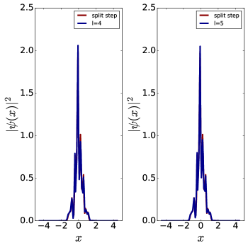
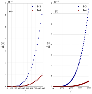
where $\mathcal{N}$ is the normalization constant. In Fig. 6.1 the comparison between the wave functions $\psi_{s}\left(x,t\right)$ and $\psi_{a}\left(x,t\right)$ is obtained by evolution starting from the initial wave function (5.3). It is presented for an arbitrary realization of the random potential (2.11). The difference is very small and it will be calculated in what follows. The results are presented in Fig 6.2 where we plot

(5.4) $$\bar{\Delta}\left(t\right)=\left\langle\Delta\left(t\right)\right\rangle_{\text{av}}.$$

The average is over 40 realizations of the potential $V\left(x,t\right)$ of (11). The averaging is performed as follows: $\Delta\left(t\right)$ is calculated for a specific realization and the average is taken so that the $\phi_{i}$ are distributed uniformly in the interval $[-\pi,\pi]$, while $v_{n}^{(r)}$ and $k_{n}$ are distributed uniformly in the intervals $[v^{min}=-15,v^{max}=15]$ and $[k^{min}=-20,k^{max}=20]$ respectively (see Sec. 2 paragraph following Eq. 5 ). $\omega_{n}$ is calculated by (2.5). We take $\beta=1\cdot 10^{-3}$ and $\beta=1\cdot 10^{-4}$ while $\sigma_{x}^{0}=1$ resulting in the initial momentum standard deviation $\sigma_{k}^{0}=0.5$. In our basis Eqs. (3.20) and (3.21) for $|\varphi_{j}^{k}>,$ the largest value of the momentum is $\left|\tilde{k}\right|=80$, therefore

(5.5) $$\left|\tilde{k}\right|\gg\sigma_{k}^{0}.$$

The largest value of $\left|x\right|$ is $10$ therefore $\sigma_{x}^{0}$ is much smaller then the largest value of $\left|x\right|$, namely 10. Note that $\Delta\left(t\right)$ is much smaller then $\delta_{a}$ and $\epsilon,$ indicating that the results are much more accurate then expected from the theoretical bounds. This may be specific to the potential we used. A similar situation was observed in the appendix of [1].

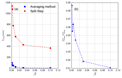
To demonstrate the efficiency of the calculation we compare the computer time $\text{T}_{\text{comp}}$ required to perform the numerical time propagation Fig. 2 up to times $t_{max}=8000$, we compare the results for the multi-scale and averaging split steps methods with the same precision $\delta_{a}=\epsilon=10^{-7}$ we choose a time $t_{max}^{{}^{\prime}}=T_{0}\cdot\bar{i}$ such that $\bar{i}$ is the smallest integer satisfying $t_{max}^{{}^{\prime}}>t_{max.}$ the lowest hierarchy $l_{min}$ required for the calculation $l$ is used. The results are summarized in table 2 and plotted in Fig 6.3. The calculations were performed on two computational nodes each composed of a 2.4 Ghz Intel Xeon processors.

$\beta$	$v$	$T_{0}^{2}$	$T_{0}^{4}$	$\delta t$ for $T_{0}^{2}$	$\delta t$ for $T_{0}^{4}$
$1\cdot 10^{-2}$	$100$	$100$	$10000$	$0.01$	$0.0009$
$1\cdot 10^{-3}$	$1000$	$1000$	$1000000$	$0.01$	$0.0001$
$5\cdot 10^{-4}$	$2000$	$2000$	$400000$	$0.009$	$*$
$1\cdot 10^{-4}$	$10000$	$10000$	$100000000$	$0.009$	*

Table 1. split step time steps for different values of the small parameter. The accuracy is $\delta_{a}=10^{-7}$

It turns out that for the problem we studied, the results we obtained are probably much better then the error estimate (4.12). To see this we present in table 3 the difference

(5.6) $$\tilde{\Delta}_{l,l+1}\left(t\right)=\int_{\Gamma}dx|\psi_{l}(x,t_{max})-\psi_{l+1}(x,t_{max})|^{2}$$

indicating the order of magnitude of the error as well as the bound (4.12) for $l=3$ and $l=4$ for different values of $\beta$ and $t_{max}=T_{0}^{2}=\frac{1}{\beta}$ Indeed this is the case. The error in the calculation of the integrand (3.2) is given by (3.35). The reason is that the matrix consisting of the $\alpha_{k_{i},k_{j}}$ is almost a unit matrix. For all of our calculations we verified that

(5.7) $$\sum_{k_{j}\neq k_{i}}^{M=64}\left|\alpha_{k_{i},k_{j}}\right|<10^{-23}$$

while

$$\sum_{k_{j}=k_{i}}^{M=64}\left|\alpha_{k_{i},k_{j}}-1\right|<10^{-20}.$$

The error in the diagonalization of the averaged Hamiltonian $\bar{H}_{j}^{\left(g\right)}$ is of the order of $10^{-50}$. The diagonalization is performed by the lancos algorithm [24].

$\beta$	$5\cdot 10^{-5}$	$1\cdot 10^{-4}$	$3\cdot 10^{-3}$	$1\cdot 10^{-2}$	$3\cdot 10^{-2}$	$1\cdot 10^{-1}$
$T_{0}$	141.42	100	18.25	10	5.77	3.162
$\begin{array}[]{c}\\ \bar{i}\end{array}$	57	81	439	801	1386	2530
$t_{max}^{{}^{\prime}}$	8061.02	8100	8015	8010	8002.07	8000.56
$l_{min}$	3	3	4	5	5	6
$T_{comp}^{av}$	93	63	50	25	8	4
$T_{comp}^{ss}$	1140	1080	780	580	420	380
$\frac{T_{comp}^{av}}{T_{comp}^{ss}}$	0.081	0.058	0.064	0.043	0.019	0.011

Table 2. The comparison between the computational time $T_{comp}^{av}$ (in minutes) using the multi-scale averaging method and the computational time $T_{comp}^{ss}$ using the split step method. Averaging over 40 realizations similar to the ones used in Fig. 2 was performed.

$\beta$	$5\cdot 10^{-5}$	$1\cdot 10^{-4}$	$3\cdot 10^{-3}$	$1\cdot 10^{-2}$	$3\cdot 10^{-2}$	$1\cdot 10^{-1}$
$\tilde{\Delta}_{3,4}$	$6\cdot 10^{-11}$	$1.04\cdot 10^{-10}$	$1.44\cdot 10^{-10}$	$1.81\cdot 10^{-10}$	$2.17\cdot 10^{-12}$	$2.5\cdot 10^{-10}$
$\epsilon_{l=3}$	$75\cdot 10^{-8}$	$3.88\cdot 10^{-7}$	$2.02\cdot 10^{-6}$	$1.78\cdot 10^{-5}$	$2.42\cdot 10^{-4}$	$2.21\cdot 10^{-3}$
$\epsilon_{l=4}$	$6.5\cdot 10^{-10}$	$1.08\cdot 10^{-9}$	$1.81\cdot 10^{-9}$	$7.5\cdot 10^{-8}$	$6.5\cdot 10^{-7}$	$8.66\cdot 10^{-5}$

Table 3. The difference (5.6) and the bound (4.12) for various values of $\beta$ and $t_{max}=T_{0}^{2}=\frac{1}{\beta}.$

6. Spreading in k-space

Multiscale and averaging (MSA) enables us to calculate very accurately the spreading in momentum space over a very long time. For this purpose we evolve the wave function $\psi\left(x,t\right)$ starting from (5.3) with $\sigma_{x}^{0}=1$ for the potential (2.11). The wave function is used to calculate the variance of the momentum

(6.1) $$\text{Var}_{k}\left(t\right)=\int\hat{\psi}^{*}\left(k,t\right)\left(k-\bar{k}\right)^{2}\hat{\psi}\left(k,t\right)dk$$

where

(6.2) $$\bar{k}=\int\hat{\psi}^{*}\left(k,t\right)k\hat{\psi}\left(k,t\right)dk$$

and $\hat{\psi}\left(k,t\right)$ is the Fourier transform of $\psi\left(x,t\right)$. Then we calculate the spread of the momentum relative to initial one

(6.3) $$\Delta\text{Var}_{k}^{\left(n\right)}\left(t\right)=\frac{\text{Var}_{k}\left(t\right)-\text{Var}_{k}\left(0\right)}{\text{Var}_{k}\left(0\right)}.$$

This calculation is performed for each realization of the random potential. Then average over 40 realizations of the random potential was performed as in (5.4), namely we calculate

(6.4) $$\bar{\Delta}_{v}\left(\tau\right)=\left\langle\Delta\text{Var}_{k}^{\left(n\right)}\left(t\right)\right\rangle_{\text{av}}$$

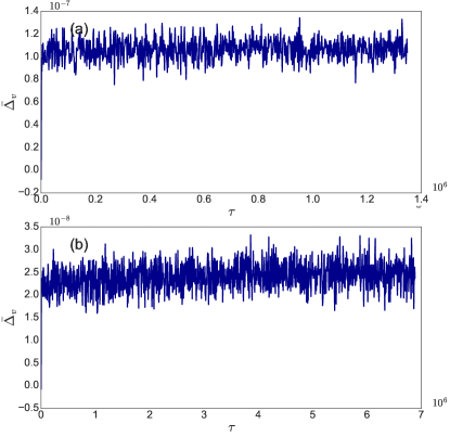
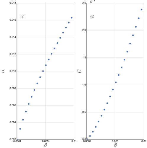
It is plotted as a function of $\tau=\beta t$ in Fig. 6.4. Because of the smallness of $\bar{\Delta}_{v}$ we conclude that the replacement of the Hamiltonian by a finite matrix does not effect the result (see Eq. (5.5)). The plot is smoothed by averaging over intervals of length $\Delta\tau=10^{2}$, leading to the results presented in Fig. 6.5, the calculation is repeated for several values of $\beta$, and in Fig. 6.6 the results are fitted to the formula

(6.5) $$\bar{\Delta}_{v}\left(\tau\right)=C\left(\beta\right)\tau^{\alpha\left(\beta\right)}.$$

From the plot it is reasonable to extrapolate

(6.6) $$\lim_{\beta\rightarrow 0}C=\lim_{\beta\rightarrow 0}\alpha=0.$$

We conclude that in the limit $\beta\rightarrow 0$ the spreading stops. This is the limit where the velocity is much larger then the Chirikov resonant velocities $v_{n}^{\left(r\right)}$ of Eq. (2.5). It leads us to the conjecture that if in one dimension the $v_{n}^{\left(r\right)}$ are bounded, the kinetic energy cannot grow to infinity, in-spite of the driving.

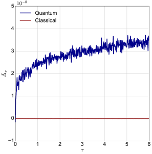
In Fig. 6.7, the classical and quantum results are compared. The quantum results were computed as the ones for Fig. 6.4 while for the classical results 60 initial conditions were also chosen at random from a Gaussian distribution corresponding to the initial quantum wave function $\psi\left(x,0\right)$ of (5.3). Both classical and quantum results were averaged over 40 realizations of the random potential. We note that both classical and quantum spreading in momentum stops. The classical spreading stops at an earlier stage.

References

• [1] S Fishman and Avy Soffer. Multiscale time averaging, reloaded. SIAM Journal on Mathematical Analysis, 46(2):1385–1405, 2014.
• [2] Liad Levi, Yevgeny Krivolapov, Shmuel Fishman, and Mordechai Segev. Hyper-transport of light and stochastic acceleration by evolving disorder. Nature Physics, 8(12):912–917, 2012.
• [3] Yevgeny Krivolapov, Liad Levi, Shmuel Fishman, Mordechai Segev, and Michael Wilkinson. Super-diffusion in optical realizations of anderson localization. New Journal of Physics, 14(4):043047, 2012.
• [4] Yevgeny Krivolapov and Shmuel Fishman. Universality classes of transport in time-dependent random potentials. Physical Review E, 86(3):030103, 2012.
• [5] Yevgeny Krivolapov and Shmuel Fishman. Transport in time-dependent random potentials. Physical Review E, 86(5):051115, 2012.
• [6] Yvon Maday, Anthony T Patera, and Einar M Rønquist. An operator-integration-factor splitting method for time-dependent problems: application to incompressible fluid flow. Journal of Scientific Computing, 5(4):263–292, 1990.
• [7] Ronnie Kosloff. Time-dependent quantum-mechanical methods for molecular dynamics. The Journal of Physical Chemistry, 92(8):2087–2100, 1988.
• [8] G. Uhlenbeck and L. Ornstein. On the theory of the brownian motion. Physical Review Letters, 36:823–841, Sep 1930.
• [9] P. Sturrock. Stochastic acceleration. Physical Review Letters, 141:186–191, Jan 1966.
• [10] CW Gardiner. Stochastic methods. Springer-Verlag, Berlin–Heidelberg–New York–Tokyo, 1985.
• [11] V. Bezuglyy, B. Mehlig, M. Wilkinson, K. Nakamura, and E. Arvedson. Generalized ornstein-uhlenbeck processes. Journal of Mathematical Physics, 47(7), 2006.
• [12] E. Arvedson, M. Wilkinson, B. Mehlig, and K. Nakamura. Staggered ladder spectra. Physical Review Letters, 96:030601, Jan 2006.
• [13] Marshall N. Rosenbluth. Comment on “classical and quantum superdiffusion in a time-dependent random potential”. Physical Review Letters, 69:1831–1831, Sep 1992.
• [14] Leonardo Golubović, Shechao Feng, and Fan-An Zeng. Classical and quantum superdiffusion in a time-dependent random potential. Physical Review Letters, 67:2115–2118, Oct 1991.
• [15] Jan S Hesthaven, Sigal Gottlieb, and David Gottlieb. Spectral methods for time-dependent problems, volume 21. Cambridge University Press, 2007.
• [16] Claude Leforestier, RH Bisseling, Charly Cerjan, MD Feit, Rich Friesner, A Guldberg, A Hammerich, G Jolicard, W Karrlein, H-D Meyer, et al. A comparison of different propagation schemes for the time dependent schrodinger equation. Journal of Computational Physics, 94(1):59–80, 1991.
• [17] Uri M Ascher, Steven J Ruuth, and Brian TR Wetton. Implicit-explicit methods for time-dependent partial differential equations. SIAM Journal on Numerical Analysis, 32(3):797–823, 1995.
• [18] Tal Schwartz, Guy Bartal, Shmuel Fishman, and Mordechai Segev. Transport and anderson localization in disordered two-dimensional photonic lattices. Nature, 446(7131):52–55, 2007.
• [19] Marie Piraud, Pierre Lugan, Philippe Bouyer, Alain Aspect, and Laurent Sanchez-Palencia. Localization of a matter wave packet in a disordered potential. Physical Review A, 83(3):031603, 2011.
• [20] Juliette Billy, Vincent Josse, Zhanchun Zuo, Alain Bernard, Ben Hambrecht, Pierre Lugan, David Clement, Laurent Sanchez-Palencia, Philippe Bouyer, and Alain Aspect. Direct observation of anderson localization of matter waves in a controlled disorder. Nature, 453(7197):891–894, 2008.
• [21] Laurent Sanchez-Palencia, David Clement, Pierre Lugan, Philippe Bouyer, Georgy V Shlyapnikov, and Alain Aspect. Anderson localization of expanding bose-einstein condensates in random potentials. Physical Review Letters, 98(21):210401, 2007.
• [22] B. V. Chirikov. A universal instability of many-dimensional oscillator systems. Physics Reports, 52(5):263 – 379, 1979.
• [23] G.M.Zaslavski. and B.V. Chirikov. Stochastic instability of non-linear oscillations. Soviet Physics Uspekhi, 14(5):549, 1972.
• [24] Richard B Lehoucq, Danny C Sorensen, and Chao Yang. ARPACK users’ guide: solution of large-scale eigenvalue problems with implicitly restarted Arnoldi methods, volume 6. Siam, 1998.