Reconstructing equation of state of dark energy with principal component analysis
Abstract
We represent a nonparametric method to reconstruct the equation of state for dark energy directly from observational Hubble parameter data. We use principal component analysis (PCA) to extract the signal from data with noise. Moreover, we modify Akaike information criterion (AIC) to guarantee the quality of reconstruction and avoid over-fitting simultaneously. The results show that our method is robust in reconstruction of dark energy equation of state. Although current observational Hubble parameter data alone can not give a strong constraint yet, our results indicate that future observations can significantly improve the quality of the reconstruction.
keywords:
Dark Energy, Reconstruction, Nonparametric Model, Observational Hubble parameter Data, Principal Component Analysis1 Introduction
Distance measurements of the type Ia supernovae (SNe Ia) indicate that the expansion of the universe is accelerating [1, 2, 3]. This implies that some mechanism must exist to provide a repulsive effect. Many theories have been proposed to explain this repulsive effect. The most popular one is the dark energy paradigm. Dark energy is one kind of special matter which can provide the repulsive force that accelerates the expansion of the universe. However, its nature still remains unclear. To study the property of dark energy, Turner and White [4] suggested to parameterize the dark energy by its equation of state, , where is pressure and is energy density. For different dark energy models, takes different values (e.g., -1 for vacuum energy, for topological defects of dimensionality ), and may also evolve with time (e.g., models with a rolling scalar field). The analysis from the Planck + WP and BICEP2 data shows that the equation of state and the bounce inflation scenario [5] is better than the standard cold dark matter model with a cosmological constant [6, 7, 8]. Although observation is consistent with and a cosmological constant [9], the possibility of a time dependence of or a coupling with cold dark matter cannot be excluded [10]. Current observational data (SNe + Planck2015 + BAO) favor the cosmological constant model [11] or XCDM and CDM models [12]. In addition, on the theoretical level a constant runs into serious problems, since the present value of is times smaller than the prediction from most particle physics models. If is not a constant, the dynamic properties of the dark energy may interest us [13, 14]. Since can well describe the dynamic properties of dark energy, it is vital to determine in the research of dark energy.
To determine the equation of state for dark energy, there are many different observational data sets that can be used. CMB anisotropy, supernovae (SNe) distance measurements and number counts all appear to be promising. One can fit directly to SNe magnitudes or their luminosity distances , or to more indirect quantities such as dark energy density, , the expansion history, [15]. But even accurate measurements of cannot constrain the small bumps and wiggles that are crucial to the reconstruction of . Without some smoothing of the cosmological measurements, the reconstruction is unfeasible [14]. As the combination of number counts and supernova measurements could determine directly and could eliminate the dependence of the second derivative of , using observational Hubble parameter data (OHD) to constrain seems to be a good choice [16].
Recently, there have been many works focusing on dark energy equation of state reconstruction. One can approach the reconstruction in a parametric or non-parametric way. Studying dark energy in a parameterized way, i.e., parameterizing the dark energy equation of state in terms of known observables [10], e.g. Chevallier-Polarski-Linder parametrization [17, 18] and divergency-free parametrizations [19], may induce biased results due to prior assumptions of function forms of the equation of state [20]. It may be more robust to reconstruct dark energy equation of state with non-parametric ways, since we do not know the nature of the dark energy so far. Reconstruction methods can also be divided into model dependent methods and model independent methods. Model dependent methods work within a particular model, while model independent methods have no such constraint. In fact, as a consequence of the strong degeneracy between cosmological models [21], any imposition would cause biased results [22]. Therefore, a reconstruction of should be carried out ideally in a model independent manner [23].
In this paper, we apply principal component analysis (PCA), which is a useful non-parametric model-independent tool, on the reconstruction of dark energy equation of state with observational Hubble parameter. However, in order to reconstruct we need to calculate the derivatives in , which can, in general, increase the errors on the reconstructed equation of state [24, 20]. To overcome this deficiency, we try to fit directly to OHD through the integral that relates to . Another problem is that PCA can determine the principal components in , but how many components one should keep is still an open question. Too many components may cause overfitting and vise versa. So we propose to modify Akaike information criterion (AIC) in order to guarantee the quality of reconstruction and avoid over-fitting.
This paper is organized as follows. First, we describe the observational Hubble parameter data and explain the generation of simulated data in section 2. Next, we present the reconstruction process of dark energy equation of state in section 3. After that, we introduce the information criterion for components selection in section 4. Then we show results in section 5. Finally, we discuss the implications of our results and draw the conclusions in section 6.
2 Observational and simulated data
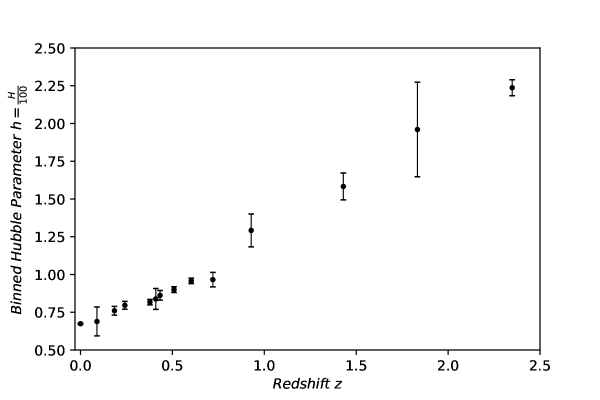
Current observational hubble parameter data are obtained primarily from the method of cosmic chronometers [25, 26, 27, 28]. Other methods to extract are by the observations of BAO peaks [29, 30] and Ly- forest of luminous red galaxies (LRGs) [31], which has extended the current OHD up to . Ref.[32, 33] provides the data set we use, which covers several independent measurements of . is set the value measured with Planck based on CMB [34], i.e., . There are data points in the data set in total ( included). As the redshift distribution of these data points is not uniform, we split the redshift region () into bins by the binning strategy in Ref.[33]. The binned observational Hubble parameter data set is shown in figure 1.
In order to validate the reconstruction process described in section 3, we use the simulated Hubble parameter data set, generated from some toy models (with known ), to reconstruct the equation of state. Then we can evaluate the quality of reconstruction through comparing reconstructed equation of state with the known .
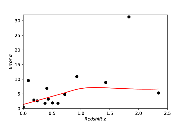
To generate a simulated Hubble parameter data set, we need a fiducial model which can be characterized by an equation of state , from which we can get the theoretical Hubble parameter via Eq. (3) with a particular . In addition to the underlying model, we also need an error model, which estimates the deviations for simulated Hubble parameter data from the theoretical values. There have been some studies on how to obtain an error model from observational Hubble parameter data. For instance, Yu et al.[20] suggested that the error of observational Hubble parameter data follow Nakagami distribution; Ma et al. [35] used the center line of upper heuristic bounds and lower heuristic bounds of the observational Hubble parameter data as the error model for simulated Hubble parameter data. Generally, the uncertainty of the observational data is strongly dependent on redshift. In this study we generate the error model for simulated Hubble parameter data by fitting the error of the observational Hubble parameter data with a lowess regression, as shown in figure 2.
Finally, with the fiducial model and the error model discussed above, we can generate the simulated Hubble parameter data via
| (1) |
where is the Gaussian distribution with zero mean and the standard deviation of the distribution is the lowess regression curve.
For each fiducial model we generate 14 simulated data points, the same number as binned OHD, with being uniformly distributed in by step 0.177.
3 Reconstructing process
We reconstruct the equation of state for dark energy with the assumption that the universe is homogeneous, isotropic and governed by Einstein’s theory of gravitation. It is well known that the metric for a space-time with homogeneous and isotropic spatial sections is the maximally-symmetric Friedmann-Robertson-Walker (FRW) metric. We also treat the whole universe as ideal fluid. Then from Friedmann equation we have
| (2) |
where is dark energy density component, is matter density component, is curvature component, and is radiation density component respectively. According to the latest result from Plank, we adopt [34]. Then Eq. 2 can be reduced to
| (3) |
from which we can calculate the theoretical Hubble parameter when the expression of is known. We can fit observational data to constrain the analytical form of through least-square method,
| (4) |
where is the number of data points, is observational or simulated Hubble parameter data, is theoretical Hubble parameter, and is the error of respectively. However, it is well known that applying Least-square minimization can not distinguish between noise and signal, as noise is included in the result of optimization. In order to minimize the effect of noise, we use PCA to determine the principal components of .
The process of applying PCA on reconstruction of equation of state is described as follows:
Step 1. We choose a set of basis functions and equation of state can be expressed as
| (5) |
where are the coefficients of the corresponding basis functions.
Step 2. We use Eq.( 3) and (4) and non-linear least-square optimization to derive the coefficients .
Step 3. We simulate enough times based on the error data (e.g. see the error bars in Fig.1), each simulation produces a different set of data. For each set of data we apply Step 2 and get one instance of . Thus we can get enough instances of , from which we calculate the covariance matrix of , denoted by C.
Step 4. We calculate the eigenvalues and eigenvectors by diagonalizing the covariance matrix C,
| (6) |
where is the diagonal matrix. The diagonal entries of are eigenvalues, and the columns of matrix are corresponding eigenvectors.
Step 5. We sort the components by in ascending order and choose first components. That is, the matrix is reduced to dimension . Then we define a new basis , where . This new basis are linear combinations of the original basis functions , and they are orthogonal. The s corresponding to small eigenvalues are the relatively stable components, which vary little for different observations. They are hence the components we need.
Step 6. Based on Eq.(3) and (4), we use the new basis functions and non-linear Least-square Optimization to fit data again and obtain the new coefficients . Finally we get equation of state
| (7) |
where is the number of used components. The covariance matrix of is just the diagonal matrix derived from Eq.(6). Besides, a criterion is needed to decide how many components (i.e. the value of ) should be used, which will be discussed in section 4.
4 Criterion for components selection
We have discussed the reconstruction process in section 3. Then we need a criterion to determine how many components we should keep in the reconstruction. This is still an open question in principal components analysis. Many criteria have been proposed to solve this problem since PCA was invented in 1901, e.g. Akaike information criterion (AIC), Bayesian information criterion (BIC) [36], and the combinations of them. Yu et al. used a criterion called Goodness of Fit [20]. Although these criteria works well in general, there are defects in these criteria: introducing either additional parameter or additional assumptions, such as in the combination of AIC and BIC [37]. Furthermore, evaluating these parameters arbitrarily may lead to quite different reconstructing results in some particular problems.
In this paper, we introduce a new criterion for principal components selection. It is a modified AICc (the small-sample-size corrected version of AIC) criterion. The expression of AICc is [38, 39]
| (8) |
where is the number of parameters, i.e. the number of components we keep, and is the size of data set. , i.e. Eq.(4), represents the deviation from observational data or simulated data. It is expected that reducing will be accompanied by a reduction in the error, but an increased chance of getting wrong [37], which means is reconstructed less accurately (so the bias increases), but the error bars are smaller (so the variance decreases)[40]. It turns out that the challenge for this issue is to achieve a balance between the bias and variance. Therefore we add an empirical parameter into the latter term of AICc to determine the value of . After that, the modified AICc criterion is
| (9) |
where is the tuning factor we add to AICc to include the penalty for more parameters and to avoid overfitting.
The introduction of parameter endows the criterion with additional flexibility, which makes it adaptable to specific problems. The value of is determined empirically and consistent with the fact that results of best fit have the minimum AICcm values. Theoretically, for the best that corresponds to minimum AICcm, the derivative of AICcm with respect to should be zero. However, this point is seldom exactly satisfied since is confined to integers. Nevertheless, we can determine the value of approximately with the help of AICcm derivative with respect to , which is shown as follows.
To stress the dependency on we rewrite Eq.(9) as
| (10) |
where . Then for one fixed we can get
| (11) |
can be taken as the proxy of right derivative of with respect to . Since get minimum at the fixed we let and get
| (12) |
Correspondingly,
| (13) |
Then the value of is calculated by
| (14) |
Hence, once the best number of components is fixed, we can calculate s through Eq. (12-14). Now we can see that the value of s and the best depends on each other: In order to calculate , the best need to be given, while the determination of the best takes as the prerequisite. To address this dilemma, we designed a iterative procedure that alteratively computes and . We initialize this procedure by set , which corresponds to AICc criterion shown in Eq. (8). In practice, this procedure can converge within 10 iterations generally. The values of , and the best for different models and OHD are listed in table 1.
5 Results
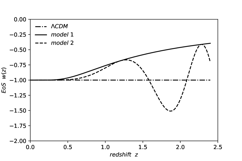
Following the reconstruction process described in section 3, we first reconstruct the equation of state from simulated Hubble parameter data generated from the fiducial model (with pre-set equation of state ). There are three we reconstruct: a. model, ; b. model-1, ; c. model-2, . Their equations of state are shown in figure 3.
The reconstruction results are shown in figure 4. It is evident that the reconstruction is reliable. Pre-set s are well in regions of reconstructed s. Furthermore, the reconstructed well recovers the trends of pre-set s up to 1.5 or so. In terms of variance, we can see the variances of reconstructed s are under control at . But at , the variances dramatically increase. The behavior of reconstructed diffs to some extent among different models. The right panel in figure 4 shows that the Hubble parameter (for convenience, we draw instead of ) calculated from reconstructed is consistent with the Hubble parameter obtained from pre-set s. And the orange region is narrow, which implies that the variance of reconstructed Hubble parameter is very small.
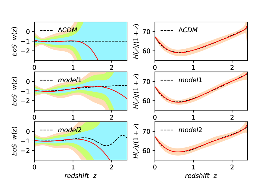
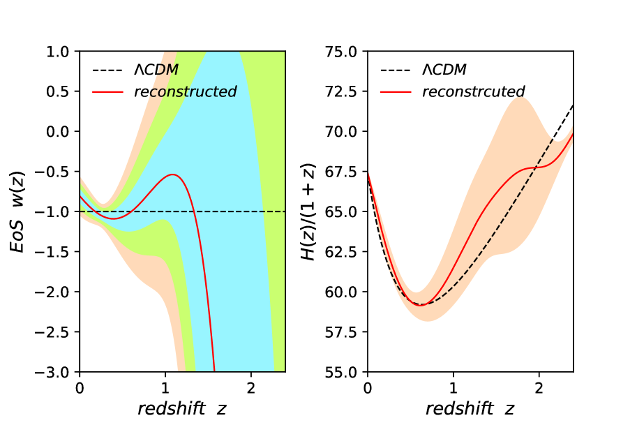
Then we reconstruct from the observational Hubble parameter data without underlying model, which is shown in Figure 5. We can see that the reconstructed oscillates around at , but at it deviates from rapidly, and the variance of it is large. Compared to the reconstructed from the simulated Hubble parameter data (Fig. 4), the OHD-reconstructed oscillates somewhat more wildly. This may be due to the fact that, compared to the observational data, the simulated redshifts are uniformly sampled and the theory values of simulated Hubble parameters, computed from the underlying model directly (through Eq.(3)), monotonically increase with . Nevertheless, combining the observational and simulated results we can conservatively conclude that the reconstruction is robust at .
6 Conclusions and discussion
We apply principal component analysis to reconstruct the dark energy equation of state. We represent as linear combination of a set of orthogonal basis functions to avoid information loss. In addition, we modify the corrected Akaike information criterion (AICc) to balance between bias and deviation in the reconstruction. Then we reconstruct the equation of state for three models from simulated Hubble parameter data to validate our reconstruction process. The results show that we can constrain the equation of state quite well at or so, and the Hubble parameter calculated from reconstructed is consistent with the Hubble parameter calculated from pre-set very well as the 1 region is very narrow. However, differences of the Hubble parameter derived from different models are very small, although the models are quite different. This is also the reason why reconstructing dark energy equation of state from Hubble parameter data is difficult. Nevertheless, from this study we show that future observations with larger quantity and higher quality of observational Hubtle parameter data will help to constrain dark energy equation of state to redshift .
Higher-redshift, more-complete-sky-coverage LRG survey and spectroscopic observations of those identified LRGs will remarkably enhance the quality of observational Hubble data. Considering a future LRG survey with more than half sky coverage, such as 2SLAQ111http://www.2slaq.info/, it may give several millions of LRGs and effectively enlarges the number of OHD data points or lowers their errors. We confirm that the ongoing CMB observation program, the Atacama Cosmology Telescope (ACT) [41], and the forthcoming surveys such as Euclid [42] and WFIRST [43] will greatly improve the present-day statistics and produce a promising dataset of larger quantity and better quality, which will result in greatly improved reconstruction of dark energy [20]. Furthermore, a small sample collected at much higher redshift, which may be implemented in near future, will reduce the errors more efficiently than collecting more events in the original redshift interval [44].
Acknowledgments
We thank Ying-Jie Peng for helpful comments and discussions. This work was supported by the National Science Foundation of China (Grants No. 11573006, 11528306), the National Key R&D Program of China (2017YFA0402600), the Natural Science Foundation of Shandong Province, China(Grant NO.ZR2019MA059), the Fundamental Research Funds for the Central Universities and the Special Program for Applied Research on Super Computation of the NSFC-Guangdong Joint Fund (the second phase).
References
- [1] S. Perlmutter, G. Aldering, G. Goldhaber, et al., Measurements of and from 42 High-Redshift Supernovae, Astrophys. J. 517 (1999) 565–586. arXiv:astro-ph/9812133, doi:10.1086/307221.
- [2] A. G. Riess, A. V. Filippenko, P. Challis, et al., Observational Evidence from Supernovae for an Accelerating Universe and a Cosmological Constant, Astron. J. 116 (1998) 1009–1038. arXiv:astro-ph/9805201, doi:10.1086/300499.
- [3] A. G. Riess, P. E. Nugent, R. L. Gilliland, et al., The Farthest Known Supernova: Support for an Accelerating Universe and a Glimpse of the Epoch of Deceleration, Astrophys. J. 560 (2001) 49–71. arXiv:astro-ph/0104455, doi:10.1086/322348.
- [4] M. S. Turner, M. White, Cdm models with a smooth component., Phys. Rev. D 56 (1997) R4439–R4443. arXiv:astro-ph/9701138, doi:10.1103/PhysRevD.56.R4439.
- [5] Y.-S. Piao, B. Feng, X. Zhang, Suppressing the cmb quadrupole with a bounce from the contracting phase to inflation., Phys. Rev. D 69 (2004) 103520.
- [6] J.-Q. Xia, H. Li, X. Zhang, Dark energy constraints after the new Planck data, Phys. Rev. D 88 (6) (2013) 063501. arXiv:1308.0188, doi:10.1103/PhysRevD.88.063501.
- [7] Z.-G. Liu, Z.-K. Guo, Y.-S. Piao, Obtaining the cmb anomalies with a bounce from the contracting phase to inflation., Phys. Rev. D 88 (6) (2013) 063539. arXiv:1304.6527, doi:10.1103/PhysRevD.88.063539.
- [8] J.-Q. Xia, Y.-F. Cai, H. Li, X. Zhang, Evidence for bouncing evolution before inflation after bicep2., Phys. Rev. Lett. 112 (25) (2014) 251301. arXiv:1403.7623, doi:10.1103/PhysRevLett.112.251301.
- [9] G. Efstathiou, W. J. Sutherland, S. J. Maddox, The cosmological constant and cold dark matter., Nature(London) 348 (1990) 705–707. doi:10.1038/348705a0.
- [10] P. S. Corasaniti, E. J. Copeland, Model independent approach to the dark energy equation of state, Phys. Rev. D 67 (6) (2003) 063521. arXiv:astro-ph/0205544, doi:10.1103/PhysRevD.67.063521.
- [11] Y.-Y. Xu, X. Zhang, Comparison of dark energy models after Planck 2015, European Physical Journal C 76 (2016) 588. arXiv:1607.06262.
- [12] J. Ooba, B. Ratra, N. Sugiyama, Planck 2015 constraints on spatially-flat dynamical dark energy models, arXiv e-printsarXiv:1802.05571.
- [13] V. Sahni, A. Starobinsky, Reconstructing dark energy., Int. J. Mod. Phys. D 15 (2006) 2105–2132.
- [14] D. Huterer, M. S. Turner, Probing dark energy: Methods and strategies., Phys. Rev. D 64 (12) (2001) 123527. arXiv:astro-ph/0012510, doi:10.1103/PhysRevD.64.123527.
- [15] R. G. Crittenden, G.-B. Zhao, L. Pogosian, L. Samushia, X. Zhang, Fables of reconstruction: controlling bias in the dark energy equation of state, JCAP 2 (2012) 048. arXiv:1112.1693.
- [16] Z.-E. Liu, H.-R. Yu, T.-J. Zhang, Y.-K. Tang, Direct reconstruction of dynamical dark energy from observational Hubble parameter data, Physics of the Dark Universe 14 (2016) 21–28.
- [17] M. Chevallier, D. Polarski, Accelerating universes with scaling dark matter., Int. J. Mod. Phys. D 10 (2001) 213–223. arXiv:gr-qc/0009008, doi:10.1142/S0218271801000822.
- [18] E. V. Linder, Exploring the expansion history of the universe., Phys. Rev. Lett. 90 (9) (2003) 091301. arXiv:astro-ph/0208512, doi:10.1103/PhysRevLett.90.091301.
- [19] J.-Z. Ma, X. Zhang, Probing the dynamics of dark energy with novel parametrizations., Phys. Lett. B 699 (2011) 233–238. arXiv:1102.2671, doi:10.1016/j.physletb.2011.04.013.
- [20] H.-R.Yu, S.Yuan, T.-J.Zhang, Nonparametric reconstruction of dynamical dark energy via observational Hubble parameter data, Phys. Rev. D 88 (10) (2013) 103528. arXiv:1310.0870, doi:10.1103/PhysRevD.88.103528.
- [21] A. Aviles, A. Bravetti, S. Capozziello, O. Luongo, Precision cosmology with Padé rational approximations: Theoretical predictions versus observational limits, Phys. Rev. D 90 (4) (2014) 043531. arXiv:1405.6935, doi:10.1103/PhysRevD.90.043531.
- [22] A. Aviles, C. Gruber, O. Luongo, H. Quevedo, Constraints from cosmography in various parametrizations., Phys. Rev. D 86 (12) (2012) 123516. arXiv:1204.2007, doi:10.1103/PhysRevD.86.123516.
- [23] O. Luongo, Cosmography with the Hubble Parameter, Mod. Phys. Lett. A 26 (2011) 1459–1466. doi:10.1142/S0217732311035894.
- [24] J.Weller, A.Albrecht, Future supernovae observations as a probe of dark energy, Phys. Rev. D 65 (10) (2002) 103512. arXiv:astro-ph/0106079, doi:10.1103/PhysRevD.65.103512.
- [25] J. Simon, L. Verde, R. Jimenez, Constraints on the redshift dependence of the dark energy potential., Phys. Rev. D 71 (2005) 123001.
- [26] D. Stern, R. Jimenez, L. Verde, S. A. Stanford, M. Kamionkowski, Cosmic Chronometers: Constraining the Equation of State of Dark Energy. II. A Spectroscopic Catalog of Red Galaxies in Galaxy Clusters, Astrophys. J. Suppl. Ser. 188 (2010) 280–289. arXiv:0907.3152, doi:10.1088/0067-0049/188/1/280.
- [27] J. Alberto Vãzquez, M. Bridges, M. P. Hobsonb, A. N. Lasenby, Reconstruction of the dark energy equation of state., J. Cosmol. Astropart. Phys. 9 (2012) 020. arXiv:1205.0847, doi:10.1088/1475-7516/2012/09/020.
- [28] C. Zhang, H. Zhang, S. Yuan, S. Liu, T.-J. Zhang, Y.-C. Sun, Four new observational H(z) data from luminous red galaxies in the Sloan Digital Sky Survey data release seven, Research in Astronomy and Astrophysics 14 (2014) 1221–1233. arXiv:1207.4541, doi:10.1088/1674-4527/14/10/002.
- [29] E. G. naga, A. Cabré, L. Hui, Clustering of luminous red galaxies c iv. baryon acoustic peak in the line-of-sight direction and a direct measurement of h(z)., Mon. Not. R. Astron. Soc. 399 (2009) 1663–1680. arXiv:0807.3551, doi:10.1111/j.1365-2966.2009.15405.x.
- [30] C. Blake, S. Brough, M. Colless, C. Contreras, W. Couch, S. Croom, D. Croton, T. M. Davis, M. J. Drinkwater, K. Forster, D. Gilbank, M. Gladders, K. Glazebrook, B. Jelliffe, R. J. Jurek, I.-h. Li, B. Madore, D. C. Martin, K. Pimbblet, G. B. Poole, M. Pracy, R. Sharp, E. Wisnioski, D. Woods, T. K. Wyder, H. K. C. Yee, The WiggleZ Dark Energy Survey: joint measurements of the expansion and growth history at z < 1, Mon. Not. R. Astron. Soc. 425 (2012) 405–414. arXiv:1204.3674, doi:10.1111/j.1365-2966.2012.21473.x.
- [31] N. G. Busca, T. Delubac, J. Rich, S. Bailey, et al., Baryon acoustic oscillations in the Ly forest of BOSS quasars, Astron. Astrophys. 552 (2013) A96. arXiv:1211.2616, doi:10.1051/0004-6361/201220724.
- [32] S.-L. Cao, H.-Y. Teng, H.-Y. Wan, H.-R. Yu, T.-J. Zhang, Testing backreaction effects with observational Hubble parameter data, European Physical Journal C 78 (2018) 170. arXiv:1704.01774, doi:10.1140/epjc/s10052-018-5616-4.
- [33] S.-L. Cao, X.-W. Duan, X.-L. Meng, T.-J. Zhang, Cosmological model-independent test of CDM with two-point diagnostic by the observational Hubble parameter data, European Physical Journal C 78 (2018) 313. arXiv:1712.01703, doi:10.1140/epjc/s10052-018-5796-y.
- [34] Planck Collaboration, N. Aghanim, Y. Akrami, et al., Planck 2018 results. VI. Cosmological parameters, arXiv e-printsarXiv:1807.06209.
- [35] C. Ma, T.-J. Zhang, Power of observational hubble parameter data: A figure of merit exploration., Astrophys. J. 730 (2011) 74. arXiv:1007.3787, doi:10.1088/0004-637X/730/2/74.
- [36] A. R. Liddle, Information criteria for astrophysical model selection., Mon. Not. R. Astron. Soc. 377 (2007) L74–L78. arXiv:astro-ph/0701113, doi:10.1111/j.1745-3933.2007.00306.x.
- [37] C. Clarkson, C. Zunckel, Direct Reconstruction of Dark Energy, Phys. Rev. Lett. 104 (21) (2010) 211301. arXiv:1002.5004, doi:10.1103/PhysRevLett.104.211301.
- [38] C. Hurvich, C.-L. Tsai, Regression and time series model selection in small samples., Biometrika 76 (1989) 297.
- [39] J. Cavanaugh, Unifying the derivations of the akaike and corrected akaike information criteria., Statistics Probability Letters 33 (1997) 201.
- [40] D.Huterer, G.Starkman, Parametrization of Dark-Energy Properties: A Principal-Component Approach, Physical Review Letters 90 (3) (2003) 031301. arXiv:astro-ph/0207517, doi:10.1103/PhysRevLett.90.031301.
- [41] http://www.physics.princeton.edu/act/index.html.
- [42] R. Laureijs, J. Amiaux, S. Arduini, et al., Euclid Definition Study Report, ArXiv e-printsarXiv:1110.3193.
- [43] D. Spergel, N. Gehrels, J. Breckinridge, et al., Wide-Field InfraRed Survey Telescope-Astrophysics Focused Telescope Assets WFIRST-AFTA Final Report, ArXiv e-printsarXiv:1305.5422.
- [44] P.Astier, Can luminosity distance measurements probe the equation of state of dark energy?, Phys. Lett. B 500 (2001) 8–15. arXiv:astro-ph/0008306, doi:10.1016/S0370-2693(01)00072-7.