The star formation history inferred from long gamma-ray bursts with high pseudo-redshifts

Abstract

By employing a simple semi-analytical star formation model where the formation rates of Population (Pop) I/II and III stars can be calculated, respectively, we account for the number distribution of gamma-ray bursts (GRBs) with high pseudo-redshifts that was derived from an empirical luminosity-indictor relationship. It is suggested that a considerable number of Pop III GRBs could exist in the present sample of Swift GRBs. By further combining the implication for the star formation history from the optical depth of the CMB photons, it is also suggested that only a very small fraction ($\sim 0.6\%$) of Pop III GRBs could have triggered the Swift BAT. These results could provide an useful basis for estimating future detectability of Pop III stars and their produced transient phenomena.

¹ School of Astronomy and Space Science, Nanjing University, Nanjing 210093, China
Email: wwtan@nju.edu.cn
² School of Physics and Electronics Information, Hubei University of Education, 430205, Wuhan, China
³ Institute of Astrophysics, Central China Normal University, Wuhan 430079, China;
Email: yuyw@mail.ccnu.edu.cn

1. Introduction

Gamma-ray bursts (GRBs), especially the major class of a duration longer than 2 seconds, are the most luminous objects in the universe, which makes them detectable even at the edge of the universe. On one hand, the reported highest redshift of GRBs so far is up to $z\sim 9.4$ for GRB 090429B (Cucchiara et al. 2011). On the other hand, some theoretical models predict that GRBs could be detected at much more distance (Band 1993; Bromm & Loeb 2006; de Souza et al. 2011). Therefore, it is widely suggested that long GRBs can be used as a cosmological tool to probe the early universe.

Long GRBs are also known to be associated with the collapse of massive stars (Galama et al. 1998; Stanek et al. 2003; Hjorth et al. 2003), which indicates that the GRB event rates could trace the cosmic star formation history either unbiasedly (e.g., Chary et al. 2007) or, more probably, with an additional evolution effect (Daigne et al. 2006; Ksitler 2008; Salvaterra 2009; Campisi et al 2010). Thanks to the launch of the Swift spacecraft, the number of GRBs with a measured redshift has been increasing rapidly during the past decade. This makes it possible to clarify the connection between the GRB numbers and the star formation rates (SFRs; e.g., Kistler et al. 2008; Cao et al. 2011; Wang & Dai 2011; Tan et al. 2013) and finally to infer the SFRs at high redshifts (Totani 1997; Wijers et al. 1998; Lamb & Reichart 2000; Porciani & Madau 2001; Murakami & Yonetoku 2005; Yüksel et al. 2008; Kistler et al. 2009; Wang & Dai 2009; Ishida et al. 2011; Wang et al. 2013) where a direct SFR-measurement is extremely difficult. Nevertheless, such attempts could somewhat be disturbed/hindered by the limited number of measured redshifts and, in particular, by some inevitable observational selection effects (Guetta & Piran 2007; Cao et al. 2011).

As an alternative and complementary method, in Tan et al. (2013), we proposed to estimate pseudo-redshifts for the Swift GRBs with an empirical relationship between the spectral peak energy and the peak luminosity. Consequently, 498 pseudo-redshifts up to $z\sim 30$ were derived from the Butler’s GRB catalog where the spectral peak energies are roughly estimated with Bayesian statistics rather than observed. Although the $L-E_{p}$ relationship is not so tight and the obtained pseudo-redshifts are not so reliable individually, a statistical study on the pseudo-luminosity distributions of the GRBs can in principle be implemented, especially worthy of mention, for different narrow redshift ranges. As a result, the luminosity function of the GRBs was found to be strongly redshift-dependent, for redshifts $z\leqslant 3.5$ and a previously-determined star formation history. From the pseudo-redshift sample of Tan et al. (2013), we can find that there are 38 GRBs whose pseudo-redshifts are higher than $10$, where 23 GRBs are above the lower luminosity cut off of Swift satellite. This statistically indicates that a remarkable number of high-redshift GRBs may exist in the present Swift GRB sample, most of which, however, evaded direct redshift measurements due to redshift selection effects.

As widely considered, for redshifts $z\gtrsim 10$, high mass Population (Pop) III stars are probably more dominant than normal Pop I/II stars (Bromm et al. 2002; Abel et al. 2002). Pop III stars were born in metal free gas and their deaths started the metal enrichment of the intergalactic medium (IGM) via supernova feedback, which subsequently lead to the formation of Pop I/II stars (Ostriker & Gnedin 1996; Madau et al. 2001; Bromm et al. 2003; Furlanetto & Loeb 2003). The high mass and zero-metallicity of Pop III stars make them easily to produce a collapsar GRB (Hirschi 2007), whose isotropically-equivalent energy could be as high as $\sim 10^{55-57}\rm ergs$ (Mészáros & Rees 2010; Suwa & Ioka 2011). Additionally, as the first generation stars in the universe, Pop III stars also turn on the cosmic reionization by emitting ultraviolet photons, and so the reionization history should strongly depend on the formation history of Pop III stars (Furlanetto & Loeb 2005; Barkana 2006; Robertson et al. 2010).

Therefore, in this paper we try to use the GRBs with high pseudo-redshifts ($z>3.5$) to probe the SFRs up to the beginning of the reionization era as well as the detection efficiency of Pop III GRBs, by combining the constraint from the optical depth of the cosmic microwave background (CMB) photons. In the next section, we will estimate the high-redshift SFRs by a usual method where the contribution to GRBs by Pop III stars is ignored, which could lead to an unacceptable result. In contrast, in section 3 we attempt to understand the GRB numbers by considering the GRB productions of both Pop I/II and III stars, where a simple semi-analytical model for the collapse of dark matter halos is employed. Finally, the results are given and discussed in section 4.

Table 1The GRB numbers in different redshift ranges.

Redshift	$N_{\rm obs}^{\dagger}$	$N_{\rm p}^{\ddagger}$
$0\sim 0.5$	10	28
$0.5\sim 1$	30	74
$1\sim 1.5$	22	96
$1.5\sim 2$	23	65
$2\sim 2.5$	20	37
$2.5\sim 3$	19	37
$3\sim 3.5$	14	24
$3.5\sim 4.5$	12	24
$4.5\sim 5.5$	5	14
$5.5\sim 6.5$	2	7
$6.5\sim 8$	2	9
$8\sim 10$	1	11
$10\sim 14$	0	12
$14\sim 18$	0	5
$18\sim 22$	0	2
$22\sim 26$	0	1
$26\sim 30$	0	3

^†GRBs of observed redshift.
^‡GRBs of a pseudo-redshift.

2. SFR-determination without Pop III stars

Table 1 lists the numbers of GRBs with observational or pseudo-redshifts for different redshift ranges, which are taken from Tan et al. (2013). Here only GRBs with luminosities higher than the lower luminosity cut off of Swift are taken into account. The difference between these two sets of numbers arises from the selection effects of redshift measurements that are, however, difficult to be described theoretically. In this paper, we will only pay attention to the numbers of pseudo-redshifts in order to probe the high-redshift ranges and avoid the redshift selection effects.

Figure 1.— SFRs inferred from the GRBs with pseudo-redshifts $>3.5$ (solid circles), where the contribution to the GRBs by Pop III stars is ignored. The crosses display the SFRs according to Hopkins & Beacom (2006) and the open diamonds correspond to the GRB-inferred SFRs given by Kistler et al. (2009). The solid (or dashed) line represents a power-law star formation history, which is required by the CMB optical depth for $N_{\gamma}=4000$ and $f_{\rm esc}=10\%$ (or $f_{\rm esc}=2\%$).

In view of the model, for a given GRB luminosity function $\Phi_{z}(L)$ and GRB event rate $\dot{R}(z)$, the expected number of GRBs within redshift range $z_{1}<z<z_{2}$ can be calculated by

$$N_{[z_{1},z_{2}]} = {\Delta\Omega\over 4\pi}T\int^{z_{2}}_{z_{1}}\int_{L_{\rm lc}(z)}\Phi_{z}(L)\dot{R}(z)dL{dV(z)\over 1+z},$$ (1)

where $\Delta\Omega/4\pi\sim 0.1$ is the field view of the Burst Alert Telescope (BAT) on board Swift, $T\sim 7\rm yr$ is the observational period, $L_{\rm lc}(z)$ is an adopted lower cutoff of the GRB luminosity corresponding to the selected data [see Equation (3) in Tan et al. (2013) and explanation therein], and $dV(z)$ is the comoving cosmic volume.

From the GRBs having a pseudo-redshift $z\leqslant 3.5$ and the corresponding star formation history

$$\dot{\rho}_{*}(z)\propto\left\{\begin{array}[]{ll}(1+z)^{3.44},~{}z\leqslant 0.97,\\ (1+z)^{0},~{}~{}~{}~{}~{}0.97<z\leqslant 3.5,\\ \end{array}\right.$$ (2)

Tan et al. (2013) derived a GRB luminosity function by:

$$\Phi_{z}(L)={1\over 4.5L_{\rm b}(z)}\left\{~{}\begin{array}[]{ll}\left({L\over L_{b}(z)}\right)^{-0.8},{}{}{}{}&L\leqslant L_{b}(z),\\ \left({L\over L_{b}(z)}\right)^{-2},{}{}{}{}&L>L_{b}(z),\end{array}\right.$$ (5)

where the break luminosity reads $L_{\rm b}(z)=1.2\times 10^{51}(1+z)^{2}\,{\rm erg}\,{\rm s}^{-1}$, and a GRB event rate as

$$\dot{R}(z)=f_{B}p(z)\dot{\rho}_{*}(z),$$ (6)

where the proportionality coefficient $f_{B}p(z)=2.4\times 10^{-8}(1+z)^{-1}M_{\odot}^{-1}$ with $f_{B}$ being the beaming factor of the GRB jets and $p(z)$ representing the GRB-production efficiency of the stars.

As the most straightforward assumption in this paper, we assume that Equations (3) and (4) are valid for all redshifts, which could be correct if all GRB progenitors belong to the same type of stars (i.e., Pop I/II stars). Then following Kistler et al. (2008, 2009), the SFRs at high redshifts can be estimated by the following equation

$$\dot{\rho}_{*}(z)\approx{N_{[z-{\Delta z\over 2},z+{\Delta z\over 2}]}\int^{3.5}_{0}\int_{L_{\rm lc}(z)}\Phi_{z}(L)p(z)\dot{\rho}_{*}(z)dL{dV(z)\over 1+z}\over N_{[0,3.5]}\int_{z-{\Delta z\over 2}}^{z+{\Delta z\over 2}}\int_{L_{\rm lc}(z)}\Phi_{z}(L)p(z)dL{dV(z)\over 1+z}}.$$ (7)

Substituting the numbers of GRBs with pseudo-redshifts for different redshift ranges into the above equation, we derive the high-redshift ($z>3.5$) SFRs as shown by the solid circles in Figure 1, where a big bump appears surprisingly in the cosmic star formation history within the redshift range $8\lesssim z\lesssim 30$.

By considering the connection between the star formation and cosmic reionization, the SFRs can also be constrained by the CMB optical depth $\tau=0.088\pm 0.015$ measured by the Wilkinson Microwave Anisotropy Probe (WMAP) experiment. Supposing a simple power-law high-redshift star formation history as $\dot{\rho}_{*}(z)\propto(1+z)^{-\alpha}$ for $z>3.5$, Yu et al. (2012) derived a constraint on the index $\alpha$ as

$$\alpha=2.18\lg(N_{\gamma}f_{\rm esc})-3.89,$$ (8)

where $N_{\gamma}$ is the number of ionizing ultraviolet photons released per baryon of the stars and $f_{\rm esc}$ is the fraction of these photons escaping from the stars. For a typical value of $N_{\gamma}\sim 4000$ for a Salpeter stellar initial mass function and a metallicity $0.05Z_{\odot}$ (e.g. Barkana 2001), we can get $\alpha=1.78$ and $0.26$, corresponding to a typical escaping fraction $f_{\rm esc}\sim 10\%$ and a very small one $f_{\rm esc}\sim 2\%$, respectively. Such requirements on the SFRs are shown by the lines in Figure 1, which are, however, significantly lower than the GRB-inferred SFRs. In other words, the SFRs simply inferred from the GRB numbers would lead to an overionized universe, unless the photon escaping fraction is unacceptably small. This indicates that something wrong must appear in the above processes of determining the SFRs by GRBs. The most probable reason could be that it is misleading to assume Equations (3) and (4) to be valid for all GRBs. In fact, for redshifts $\gtrsim 10$, Pop III stars could play a dominant role in producing GRBs. Due to the unique properties of Pop III stars, the formation history of Pop III GRBs is probably very different from that of Pop I/II GRBs. In such a case, one may worry whether the Pop III GRBs can obey the same $L-E_{p}$ relationship as Pop I/II GRBs. In our opinion, the $L-E_{p}$ relationship is probably determined by the emission mechanism of the GRB jets, which could not be sensitive to the progenitor properties.

3. Confronting the GRB numbers with a star formation model

3.1. Semi-analytical star formation model

In the hierarchical formation model, star formation takes place during the collapsing and merging of dark matter halos. A straightforward semi-analytical approach for the abundance of dark halos was first given by the Press-Schechter (PS) formalism (Press & Schechter 1974), which was subsequently improved by Sheth & Tormen (1999). By using the Sheth-Tormen mass function (ST) $n_{\rm ST}(M,z)$ of dark halos, the collapse fraction of mass available for star formation can be calculated by

$$f_{\rm col}(z)=\int_{M_{\min}}^{\infty}n_{\rm ST}(M,z){M\over\bar{\rho}}dM,$$ (9)

where $\bar{\rho}$ is the mean density of the universe and $M_{\min}$ is the minimum mass of the halos below which the halos can not collapse. By requiring the virial temperature $T_{\rm vir}$ of the halos to be higher than the temperature permitted by possible cooling channels, the minimum halo mass can be determined to $M_{\min}\sim 10^{8}{\rm M_{\odot}}\left({T_{\rm vir}/10^{4}\rm K}\right)^{3/2}\left[{(1+z)/10}\right]^{-3/2}$. Here we typically assume the minimum halo mass corresponds to the virial temperature of $T_{\rm vir}=10^{4}$ both for Pop I/II and Pop III stars, above which atomic hydrogen cooling is effective.

The star forming halos (“galaxies”) could launch a wind of metal-enriched gas with an initial speed of $v_{\rm 0}$ by producing a large number of supernovae. The well-known Sedov (1959) solution predicts that the galactic wind could travel a comoving distance of $R_{\rm w}=v_{\rm w}t=(3E_{\rm w}/2\pi f_{b}{\rho})^{1/5}t^{2/5}$, where $v_{\rm w}$ is the average wind speed while traveling in the apace, $\rho$ is the density, $E_{\rm w}={1\over 2}f_{*}f_{\rm w}f_{b}Mv_{\rm 0}^{2}$ is the total energy of the galactic wind with $f_{b}=0.167$ being the mass fraction of baryonic matter, $f_{*}$ the star formation efficiency, and $f_{\rm w}$ the energy fraction that goes into the wind. Here we have assumed that each wind has propagated for half of the age of the universe with ${\rm t}\approx 1/3H(z)$. Therefore, the volume-filling fraction of the metal-enriched gas of a collapsing halo can be expressed by $\eta(M,z)=(R_{\rm w}/R_{h})^{3}$, where $R_{h}=(3M/720\pi\bar{\rho})^{1/3}$ is the radius of the whole halo (e.g. Johnson 2010). Then, by considering the mass distribution of the halos, the total fraction of the cosmic volume that is metal-enriched by the galactic winds can be written as (Furlanetto & Loeb 2005; Greif & Bromm 2006)

$$Q_{e}(z)=[1+\xi_{\rm hh}(z)]\int_{M_{\min}}^{\infty}\eta(M,z)n_{\rm ST}(M,z){M\over\bar{\rho}}dM,$$ (10)

where $\xi_{\rm hh}(z)$ is the linear correlation function between two halos with mass M at a comoving distance R:

$$\xi_{\rm hh}(M,R,z)=b^{2}(M,z)\xi_{\rm mm}(R),$$ (11)

here $b(M,z)$is the linear bias of a halo and $\xi_{\rm mm}(R)$ is the mass correlation function (e.g. Mo $\&$ White 2002) with $R$ being the average wind size in the comoving unites. The average bias of the enriched regions is given by,

$$\bar{b}(z)={\int^{\infty}_{M_{\rm min}}{\rm d}MM\eta(M,z)b(M,z)n_{\rm ST}\over\int^{\infty}_{M_{\rm min}}{\rm d}MMn_{\rm ST}}.$$ (12)

By assuming that the host galaxies were randomly distributed, we could get the enrichment probability $p_{e}=1-{\rm exp}[-Q_{e}(z)]$.

Since the halos hosting zero-metallicity Pop III stars should not be located in the wind radius of old galaxies, the SFR of Pop III stars at redshift $z$ can be roughly estimated by

$$\dot{\rho}_{*}^{\rm III}(z)=f_{*}^{\rm III}f_{b}\bar{\rho}(1-p_{e}){{df_{\rm col}}\over dz}{dz\over dt},$$ (13)

where $f_{*}^{\rm III}$ is the fraction of baryonic mass that goes into Pop III stars. Simultaneously, the SFR of Pop I/II stars read

$$\dot{\rho}_{*}^{\rm I/II}(z)=f_{*}^{\rm I/II}f_{b}\bar{\rho}p_{e}{{df_{\rm col}}\over dz}{dz\over dt},$$ (14)

where $f_{*}^{\rm I/II}$ is the baryonic fraction for Pop I/II star formation.

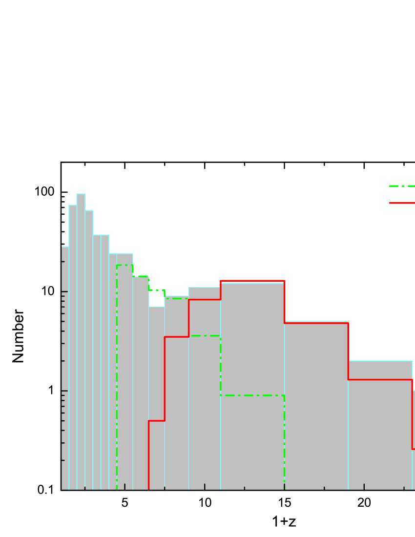
Figure 2.— Fitting to the number distribution of the GRBs with pseudo-redshifts (grey histograms) by combining the contributions to GRB productions from Pop I/II (dash-dotted line) and III (solid line) stars.

3.2. Fitting to the GRB number distribution

Different from the treatment in Section 2, here we assume the GRB luminosity function presented in Eq. (3) and the connection between the GRB event rate and SFR in Eq. (4) are only valid for the GRBs produced by Pop I/II stars. Instead of Eq. (1), we calculate the number of Pop III GRBs within redshift range $z_{1}<z<z_{2}$ by the following formula:

$$N^{\rm III}_{[z_{1},z_{2}]} = {\Delta\Omega\over 4\pi}T\zeta\int^{z_{2}}_{z_{1}}\dot{R}^{\rm III}(z){dV(z)\over 1+z}dz$$ (15)

with $\dot{R}^{\rm III}(z)=f_{B}p^{\rm III}{\dot{\rho}_{*}^{\rm III}(z)}$, where the parameter $\zeta$ represents the detection efficiency of Pop III GRBs (see discussions at the end of Section 3.3) and the GRB-production efficiency of Pop III stars $p^{\rm III}$ is considered to mainly arise from the mass requirement on the progenitors. The masses of Pop III stars are usually considered to be higher than $100\rm M_{\odot}$ (Bromm et al. 2002; Abel et al. 2002), but a much lower mass as $\sim 10\rm M_{\odot}$ was also suggested by some recent more elaborate researches where the feedback effects are taken into account simultaneously (Greif & Bromm 2006; de Souza 2011; Hosokawa et al. 2011, 2012; Stacy et al. 2012). In such a case, there could be only a small fraction of Pop III stars available for GRB production, because the GRB production could require the progenitor’s mass higher than $\sim 40\rm M_{\odot}$ (Belczynski et al. 2007; Tornatore et al. 2007; Marassi 2009). In addition, it is widely suggested that Pop III stars with masses $140\rm M_{\odot}\lesssim m\lesssim 260M_{\odot}$ would be completely disrupted by a supernova explosion due to the pair-creation instability (PISN; Heger & Woosley 2002), so they also can not contribute to GRBs. Finally, by invoking the Salpeter mass function $\phi(m)$, the GRB production efficiency of Pop III stars can be estimated by $p^{\rm III}=\left.\left[\int_{40M_{\odot}}^{140M_{\odot}}\phi(m)dm+\int_{140M_{\odot}}^{10^{3}M_{\odot}}\phi(m)dm\right]\right/\int_{10M_{\odot}}^{10^{3}M_{\odot}}M\phi(m)dm=4\times 10^{-3}\rm M_{\odot}^{-1}$.

Substituting Eq. (12) into (1) and Eq. (11) into (13), we can calculate the numbers of Pop I/II and III GRBs, respectively, for specific values of model parameters. By confronting these model-predicted GRB numbers with the numbers listed in Table 1, we can in principle obtain an observational constraint on the model parameters. We firstly take typical values for some parameters according to some previous works as $T_{\rm vir}=10^{4}$ K for atomic hydrogen cooling (Haiman et al. 2000; Furlanetto & Loeb 2005), $f_{\rm w}=0.1$ (e.g., Scannapieco & Broadhursts 2001; Springel & Hernquist 2003; ), and $v_{0}=200\rm km/s$ (Fabian et al. 1980; Eymeren et al. 2007). For the remaining more uncertain parameters $f_{*}^{\rm I/II}$, $f_{*}^{\rm III}$, and $\zeta$, their best-fit values are constrained to $f_{*}^{\rm I/II}=0.16$ and $f_{*}^{\rm III}\zeta=6\times 10^{-6}$ by fitting to the GRB number distribution without error bars. The corresponding fitting is shown in Figure 2 by the lines. The value of $f_{*}^{\rm I/II}$ could be well consistent with some previous analytical estimations and simulations (Greif & Bromm 2006; Marassi et al. 2009). Qualitatively, our result indicates that (i) the formation history of Pop I/II stars with typical values of parameters is basically favored by the GRB numbers, and (2) a considerable number of Pop III GRBs could exist in the present Swift GRBs although the degeneracy between $\zeta$ and $f_{*}^{\rm III}$ has not been removed.

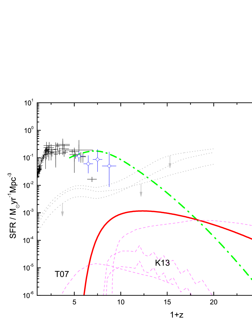
Figure 3.— High-redshift star formation history of Pop I/II (dash-dotted line) and III stars (solid line), which are constrained by the GRB numbers and the CMB optical depth together. For comparisons, some simulation results of the formation history of Pop III stars are also presented by dashed lines, such as Tornatore et al. (2007; T07), Trenti & Stiavelli (2009; TS09), and Kulkarni et al. (2013; K13). The dotted lines with arrows give an upper limit on the SFRs of Pop III stars, which is taken from Inoue et al. (2013).

3.3. Cosmic reionization

In order to remove the degeneracy between the parameters $\zeta$ and $f_{*}^{\rm III}$, we further invoke an implication for the star formation history from the CMB optical depth. The evolution of the cosmic reionization denoted by $x\equiv n_{\rm H~{}II}/n_{\rm H}$ can be determined by the following equation

$${dx\over dz}=\left[{\dot{n}_{\gamma}\over(1+y)n_{\rm H}^{0}}-\alpha_{B}C(z)(1+z)^{3}(1+y)n_{\rm H}^{0}x\right]{dt\over dz}$$ (16)

with a rate of ionizing ultraviolet photons escaping from stars into IGM $\dot{n}_{\gamma}(z)=N_{\gamma}f_{\rm esc}{\dot{\rho}_{*}(z)/m_{B}}$, where $m_{B}$ is the mass of a baryon. $y=0.08$ by assuming that the helium was only once ionized, $n_{\rm H}^{0}=1.9\times 10^{-7}~{}\,\rm cm^{-3}$ is the local number density of hydrogen, $\alpha_{B}=2.6\times 10^{-13}\,\rm cm^{3}\,{\rm s}^{-1}$ is the recombination coefficient for electron temperature of about $10^{4}K$, and $C(z)=2.9\left[{(1+z)/6}\right]^{-1.1}$ (or $=2.9$) for $z>5$ (or $z\leqslant 5$) is the clumping factor of ionized gas. With a given reionization history $x(z)$, the CMB optical depth can be calculated by integrating the electron density times the Thomson cross section along proper length as

$$\tau=-(1+y)\sigma_{T}n_{\rm H}^{0}c\int_{0}^{z_{h}}(1+z)^{3}x(z){dt\over dz}dz.$$ (17)

Here we define the upper limit of the integral to be a moderate value with $z_{h}\sim 30$, because the CMB optical depth could be mainly contributed by the electrons at relatively low redshifts $z\ll z_{h}$, and also as the WMAP experiment is insensitive to too high redshifts (Larson et al. 2011).

In the star formation model with the parameters constrained above, the remaining free parameter $f_{*}^{\rm III}$ can be determined to be $f_{*}^{\rm III}=10^{-3}$ from the CMB optical depth $\tau=0.088$, where we take $f^{\rm I/II}_{\rm esc}=6\%$, $N_{\gamma}^{\rm I/II}=4000$, $f^{\rm III}_{\rm esc}=30\%$, and $N_{\gamma}^{\rm III}=3\times 10^{4}$ (Greif & Bromm 2006). Such a value is just located within its theoretically-expected range of $\sim 10^{-6}-10^{-3}$ (Greif & Bromm 2006; Marassi et al. 2009). At the same time, the detection efficiency of Pop III GRBs is revealed to be $\zeta=0.6\%$. Such a low efficiency could be caused by various reasons. For example, the luminosity selection with an unknown luminosity function of Pop III GRBs should be included in the parameter $\zeta$, and some Pop III GRBs might occur in extremely dense accretion envelopes that suppress the GRB luminosity at early times. Moreover, the high gamma-ray variability of the GRBs could be significantly smoothed by the high redshifts, which could lead to facilities such as Swift BAT not to be triggered by the gamma-ray emission.

4. Results and Discussions

The star formation histories of Pop I/II and III stars with the obtained parameter values are presented in Figure 3. Firstly, the SFRs at redshift range $5\lesssim z\lesssim 10$ are suggested to be slightly higher than the ones given by Kistler et al. (2009), because here an evolving GRB luminosity function is adopted for Pop I/II GRBs and a larger GRB number with pseudo redshift is used here. Secondly, the formation history of Pop III stars is demonstrated to be basically consistent with some previous simulations and an observational upper limit is derived from the gamma-ray attenuations. To be specific, the peak of the SFRs of Pop III stars appears from our analysis to be at $z\sim 11$ and the formation of Pop III stars could continue down to as low as $z\sim 5$. The transition from the formation of Pop III stars to Pop I/II stars takes place at $z\sim 18$. Finally, although the simple star formation model can account for the GRB numbers for a wide redshift range as $z\lesssim 25$, the GRB number for $26<z<30$ still significantly exceeds the model prediction. Such an obvious excess may indicate some other GRB origins in the early universe, e.g., superconducting cosmic strings (Cheng et al. 2010). In this paper, we do not provide a precise regression analysis of the data, by considering that the large intrinsic uncertainty of the present pseudo-redshift data makes it unnecessary to find a high-precision fitting. In the future, a more accurate method to get the GRB pseudo-redshift is expected.

The determination of the SFRs of Pop III stars is of fundamental importance for estimating the detection efficiencies of these stars and their produced transient phenomena with some future facilities. For example, the upcoming James Webb Space Telescope (JWST) is expected to be able to detect the supernovae of Pop III stars up to $z\sim 50$, especially the PISN (Mackey et al. 2003; Weinmann & Lilly 2005). For the Pop III GRBs, their radio afterglows may also be observable by SKA, EVLA, LOFAR, and ALMA in the future (de Souza et al. 2011). Such an afterglow observation could provide a more direct test on the gamma-ray detection efficiency ($\zeta$) of the GRBs.

References

- (1) Abel, T., Bryan, G. L., & Norman, M. L. 2002, Science, 295, 93
- (2) Band, D., Matteson, J., Ford, L. et al. 1993, ApJ, 413, 281
- (3) Barkana, R., & Loeb, A. 2001, Phys. Rep., 349, 125
- (4) Barkana, R. 2006, Science, 313, 931
- (5) Belczynski, K., Bulik, T., Heger, A. and Fryer, C. 2007, ApJ, 664, 986
- (6) Bromm, V., Coppi, P. S., Larson, R. B. 2002, ApJ, 564, 23
- (7) Bromm, V., Loeb, A. 2003, Nature, 425, 812
- (8) Bromm, V., Loeb, A. 2006, ApJ, 642, 382
- (9) Campisi, M. A., Li, L.-X., Jakobsson, P. 2010, MNRAS, 407, 1972
- (10) Cao, X. F., Yu, Y. W., Cheng, K. S., & Zheng, X. P. 2011, MNRAS, 416, 2174
- (11) Chary, R.-R., Berger, E., & Cowie, L. 2007, ApJ, 671, 272
- (12) Cheng, K. S., Yu, Y. W., & Harko, T. 2010, PRL, 104, 241102
- (13) Cucchiara, A., Levan, A. J., Fox, D. B., et al. 2011, ApJ, 736, 7
- (14) Daigne, F., Tossi, E. M., Mochkovitch, R. 2006, MNRAS, 372, 1034
- (15) de Souza, R. S., Yoshida, N., Ioka, K. 2011, A&A, 533, 32
- (16) Fabian, A. C., Nulsen, P. E. J., & Stewart, G. C. 1980, Nature, 287, 16
- (17) Furlanetto, S. R., Loeb, A. 2005, ApJ, 634, 1
- (18) Furlanetto, S. R., Loeb, A. 2003, ApJ, 588, 18
- (19) Galama, T. J., Vreeswijk, P. M., van Paradijs, J., et al. 1998, Nature, 395, 670
- (20) Greif, T., H., & Bromm, v. 2006, MNRAS, 373, 128
- (21) Guetta, D., & Piran, T. 2007, JCAP, 07, 003
- (22) Haiman, Z., Abel, T., Rees, M. J. 2000, ApJ, 534, 11
- (23) Heger, A., Woosley, S. E. 2002, ApJ, 567, 532
- (24) Hirschi, R. 2007, A&A, 461, 571
- (25) Hjorth, J., Sollerman, J., Mller, P., et al. 2003, Nature, 423, 847
- (26) Hopkins, A. M., Beacom, J. F. 2006, ApJ, 651, 142
- (27) Hosokawa, T., Omukai, K., Yoshida, N., Yorke, H. W. 2011, Science, 334, 1250
- (28) Hosokawa, T., Yoshida, N., Omukai, K., Yorke, H. W. 2012, ApJL, 760, L37
- (29) Inoue, Y., Tanaka, Y. T., Madejski, G. M. et al. 2013, arxiv: 1312. 6462
- (30) Ishida, E. E. O., de Souza, R. S., & Ferrara, A. 2011, MNRAS, 418, 500
- (31) Johnson, J. L. 2010, MNRAS, 404, 1425
- (32) Kistler, M. D., Yksel, H., Beacom, J. F., Stanek, K. Z. 2008, ApJL, 673, L119
- (33) Kistler, M. D. et al. 2009, ApJL, 705, L104
- (34) Kulkarni, G., Rollinde, E., Hennawi, J. F., Vangioni, E. 2013, arXiv:1301.4201
- (35) Lamb, D. Q., & Reichart, D. E. 2000, ApJ, 536, 1
- (36) Larson, D., Dunkley, J., Hinshaw, G., Komatsu, E., Nolta, M. et al. 2011, Astrophys. J. Suppl., 192, 16
- (37) Mackey, J., Bromm, V., & Hernquist, L. 2003, ApJ, 586, 1
- (38) Madau, P., Rees, M. J. 2001, ApJL, 551, L27
- (39) Marassi, S., Schneider, R. & Ferrari V. 2009, MNRAS, 398, 293
- (40) Mészáros, P. & Rees, M. J. 2010, ApJ, 715, 967
- (41) Mo, H. J. & White, S. D. M. 2002, MNRAS, 336, 112
- (42) Murakami, T., & Yonetoku, D. 2005, ApJL, 625, L13
- (43) Ostriker, J. P., Gnedin, N. Y. 1996, ApJL, 472, L63
- (44) Porciani, C., & Madau, P. 2001, ApJ, 548, 522
- (45) Press, W. H., Schechter, P. 1974, ApJ, 187, 425
- (46) Robertson, B. E., Ellis, R. S., Dunlop, J. S., McLure, R. J., & Stark, D. P. 2010, Nature, 468, 49
- (47) Salvaterra, R., Guidorzi, C., Campana, S., Chincarini, G., Tagliaferri, G. 2009, MNRAS, 396, 299
- (48) Scannapieco, E., & Broadhurst, T. 2001, ApJ, 549, 28
- (49) Springel, D. N., Hernquist, L. 2003, MNRAS, 339, 312
- (50) Sheth, R. K., Tormen, G. 1999, MNRAS, 308, 119
- (51) Stacy, A., Greif, T. H., & Bromm, V. 2012, MNRAS, 422, 290
- (52) Stanek, K. Z., Matheson, T., Garnavich, P. M., et al. 2003, ApJL, 591, L17
- (53) Suwa, Y. & Ioka, K. 2011, ApJ, 726, 107
- (54) Tan, W. W., Cao, X. F., & Yu, Y. W. 2013, ApJL, 772, L8
- (55) Tornatore, L., Ferrara, T., & Schneider, R. 2007, MNRAS, 382, 945
- (56) Totani, T. 1997, ApJL, 486, L71
- (57) Trenti, M. & Stiavelli, M. 2009, ApJ, 694, 879
- (58) van Eymeren, J., Bomans, D. J., Weis, K. & Dettmar R. J. 2007, A&A, 474, 67
- (59) Wang, F. Y. & Dai, Z. G. 2009, MNRAS, 400, L10
- (60) Wang, F. Y. & Dai, Z. G. 2011, ApJ, 727, L34
- (61) Wang, F. Y. 2013, A & A, 556, A90
- (62) Weinmann, S. M., & Lilly, S. J. 2005, ApJ, 624, 526
- (63) Wijers, R. A. M., Bloom, J. S., Bagla, J. S., & Natarajan, P. 1998, MNRAS, 294, L13
- (64) Yu, Y. W., Cheng, K. S., Chu, M. C., & Yeung, S. 2012, JCAP, 07, 023
- (65) Yüksel,H., Kistler, M. D., Beacom, J. F., & Hopkins, A. M. 2008, ApJ, 683, L5