The SMC’ is a highly accurate approximation to the ancestral recombination graph

Abstract

Two sequentially Markov coalescent models (SMC and SMC’) are available as tractable approximations to the ancestral recombination graph (ARG). We present a Markov process describing coalescence at two fixed points along a pair of sequences evolving under the SMC’. Using our Markov process, we derive a number of new quantities related to the pairwise SMC’, thereby analytically quantifying for the first time the similarity between the SMC’ and ARG. We use our process to show that the joint distribution of pairwise coalescence times at recombination sites under the SMC’ is the same as it is marginally under the ARG, which demonstrates that the SMC’ is, in a particular well-defined, intuitive sense, the most appropriate first-order sequentially Markov approximation to the ARG. Finally, we use these results to show that population size estimates under the pairwise SMC are asymptotically biased, while under the pairwise SMC’ they are approximately asymptotically unbiased.

1 Introduction

Of the many models of genetic variation in the field of population genetics, few have as much relevance in the era of genomics as the ancestral recombination graph (ARG). The ancestral recombination graph models patterns of ancestry and genetic variation within sequences experiencing recombination under neutral conditions (Hudson, 1991; Griffiths and Marjoram, 1997). Under the formulation of Griffiths and Marjoram (1997), lineages recombine apart and coalesce together back in time to produce a graph structure describing the ancestral genealogy at each point along a continuous chromosome. While only a few simple rules govern the process, many aspects of the model are analytically intractable.

Wiuf and Hein (1999) provided a formulation of the ARG that proceeds across the chromosome (rather than back in time), producing the genealogy at each point sequentially. As with the back-in-time formulation of the ARG, at each point along the chromosome there is a local genealogy describing the ancestry of the sample at that point, and changes in the genealogy occur at recombination sites. In this sequential formulation of the ARG, a new lineage is produced wherever an ancestral recombination event is encountered along the chromosome. To produce a new genealogy at the recombination site, the new lineage is coalesced to the ARG representing the ancestry of all previous points along the chromosome. This dependence on all previous points makes the process non-Markovian along the chromosome and (together with a large state space) makes calculations often intractable.

Approximations to the ARG have been suggested with the goal of modeling coalescence with recombination in a way that is analytically tractable. McVean and Cardin (2005) introduced the sequentially Markov coalescent (SMC). The original formulation of the SMC was sequential, generating genealogies along the chromosome such that each new genealogy depends only on the previous genealogy. Like the ARG, the SMC has both a back-in-time formulation and a sequential formulation. The back-in-time formulation of the SMC is equivalent to that of the ARG except that coalescence is allowed only between lineages containing overlapping ancestral material. As a consequence, in the sequential formulation of the pairwise (${n=2}$ chromosomes) SMC, each recombination event produces a new pairwise coalescence time.

Marjoram and Wall (2006) introduced a slight modification to the SMC, termed the SMC’, which retains the Markov behavior along the chromosome but models additional coalescence events that make it a closer approximation to the ARG. Specifically, in the back-in-time formulation of the SMC’, coalescence is allowed between lineages containing either overlapping or adjacent ancestral material. In the sequential formulation of the pairwise SMC’, this means that not every recombination event necessarily produces a new pairwise coalescence time, since two lineages created by a recombination event can coalesce back together. Figure 1 shows the transitions that are permitted under the back-in-time and sequential formulations of the pairwise ARG, SMC, and SMC’. The sequentially Markov coalescent models have been used in many recently introduced population-genetic, model-based inference procedures, including the pairwise SMC (PSMC) model (Li and Durbin, 2011), multiple SMC (MSMC) model (Schiffels and Durbin, 2014), diCal (Sheehan et al., 2013), coalHMM (Hobolth et al., 2007; Dutheil et al., 2009), ARGWeaver (Rasmussen et al., 2014), and in a study of past human demography based on tracts of identity by state (Harris and Nielsen, 2013).

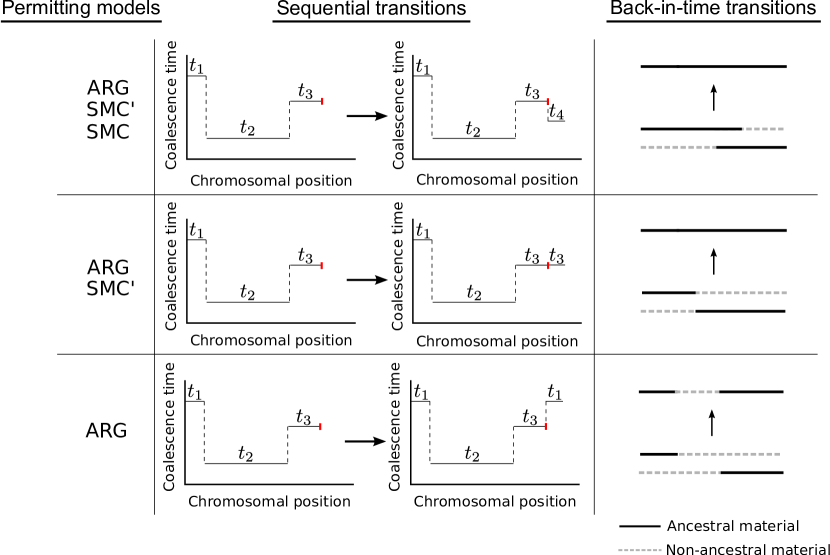
Figure 1: Transitions permitted under the pairwise ARG, SMC’, and SMC models. Under “Sequential Transitions,” a transition occurs left to right across the chromosome at the rightmost recombination event (marked with red line). The $i$th coalescence time is labeled as $t_{i}$. Under “Back-in-time transitions,” the arrow indicates a coalescence event that occurs between two aligned ancestral chromosomes, each carrying a combination of ancestral (solid black lines) and non-ancestral material (dashed gray lines). Ancestral material is defined as a portion of a chromosome that is ancestral to the sample.

The SMC’ was shown by simulation to produce measurements of linkage disequilibrium more similar to the ARG than those produced by the SMC (Marjoram and Wall, 2006), and was hence used as the preferred model by some recent studies (Harris and Nielsen, 2013; Schiffels and Durbin, 2014; Zheng et al., 2014). Additionally, a number of recent studies have explored the theoretical properties of the SMC’ (Eriksson et al., 2009; Harris and Nielsen, 2013; Carmi et al., 2014; Schiffels and Durbin, 2014; Zheng et al., 2014). However, few direct comparisons between the SMC’ and the ARG have been made, and there remain a number of open questions. Here, we show how the joint distribution of pairwise coalescence times at two fixed points along a chromosome evolving under the SMC’ can be described by a continuous-time Markov chain. Through analysis of this Markov chain, we calculate many statistical properties of the pairwise SMC’ and compare them to those of the ARG and SMC. Specifically, for each model of coalescence with recombination, we compare the following: the joint density ${f_{T_{1},T_{2}}(t_{1},t_{2})}$ (Section 2.2), the conditional density ${f_{T_{2}|T_{1}}(t_{2}|t_{1})}$ (Section 2.3), and the covariance between $T_{1}$ and $T_{2}$, which we show to be equal to the probability that $T_{1}$ and $T_{2}$ are the same (Section 2.4). These quantities are readily related to measures of linkage disequilibrium in real sequence data.

Using our two-locus Markov process for the two-locus, pairwise SMC’, we also show that the joint distribution of coalescence times immediately to the left and right of a recombination event is the same under the SMC’ and ARG. This allows us to calculate the asymptotic bias of the pairwise SMC- and SMC’-based population-size estimators, which we confirm by simulation. We show that the SMC’ estimator is approximately asymptotically unbiased.

2 Results

2.1 Two-locus Markov chain model for the SMC and SMC’

Here, we present back-in-time Markov processes for the two-locus SMC and SMC’. Previous work has developed analogous two-locus, back-in-time Markov processes for the ARG. Kaplan and Hudson (1985) first described how the process of generating coalescence times at two linked loci modeled by the ARG can be represented as a continuous-time Markov chain, with coalescence and recombination events causing transitions between states. Simonsen and Churchill (1997) explored this process further for the case where the sample size is $n=2$ and derived for the ARG many of the quantities we compare against the SMC’ in this paper. Subsequent work has extended this approach to study two-locus coalescence distributions in the presence of population structure (Eriksson and Mehlig, 2004) and recurrent bottlenecks (Schaper et al., 2012), and to study species-tree concordance at linked loci (Slatkin and Pollack, 2006) and coalescence histories at one locus conditional on the history at a nearby locus (Hobolth and Jensen, 2014).

We begin by presenting the simpler SMC model, which will provide context for the more-complex SMC’ model. If time is scaled such that the rate of coalescence is $1$ and the total rate of recombination between the two linked loci is $\rho/2$, then the two-locus ancestral process under the SMC is the process depicted in Figure 2. The process starts in state $\boldsymbol{R_{0}}$ with two lineages, each containing linked copies of the two loci. From $\boldsymbol{R_{0}}$, the process transitions with rate $\rho$ to state $\boldsymbol{R_{1}}$, in which one of the two chromosomes has experienced a recombination event, or with rate $1$ to state $\boldsymbol{C_{B}}$, an absorbing state in which both loci have coalesced. Under the SMC, lineages can only coalesce if they contain overlapping ancestral material, so after entering $\boldsymbol{R_{1}}$, the process cannot return to the fully linked state $\boldsymbol{R_{0}}$, and each locus coalesces independently with rate $1$ from that time onward. Thus, under the SMC, the joint distribution of coalescence times at two loci is that of

$$(T_{1},T_{2})\sim(X_{0}+RX_{L},\ X_{0}+RX_{R}),$$ (1)

where $X_{0}\sim\operatorname{Exp}(1+\rho)$ is the amount of time to leave $\boldsymbol{R_{0}}$, $R\sim\operatorname{Bernoulli}(\frac{\rho}{1+\rho})$ indicates whether the first event is a recombination event, and $X_{L}\sim X_{R}\sim\operatorname{Exp}(1)$ are the exponential waiting times until coalescence after the first recombination event. All of these random variables are independent in the SMC model, so it is straightforward to calculate many of the quantities we compare in this paper using this representation.

The defining rule of the SMC’ model of coalescence with recombination is that only ancestral lineages containing overlapping or contiguous ancestral material can coalesce (Marjoram and Wall, 2006). The back-in-time process of coalescence at two fixed loci under this model is the continuous-time Markov chain shown in Figure 3. Under the SMC’, it is necessary to model the number of recombination events that have occurred between the two loci at each point in time. To see that this is the case, consider the state $\boldsymbol{R_{2}}$ in Figure 3. In this state, two recombination events have occurred between the focal loci, and neither focal locus has coalesced. Because lineages can only coalesce to lineages containing overlapping or adjacent ancestral material, two particular coalescence events would need to occur before the process returns to state $\boldsymbol{R_{0}}$, regardless of the placement of the recombination events on the two chromosomes.

The SMC’ two-locus Markov process also features an additional state $\boldsymbol{I}$, which is entered when some portion of the chromosome between the focal loci coalesces before either of the focal loci. Upon entering $\boldsymbol{I}$ it becomes impossible for the process to re-enter the initial, fully-linked state ($\boldsymbol{R_{0}}$), so the remaining times until coalescence at the focal loci become independent exponential random variables with mean $1$. If $\boldsymbol{R_{i}}$ is the state in which neither focal locus has coalesced and $i$ recombination events have occurred between the focal loci, the transition rate into $\boldsymbol{I}$ is $i-1$. This is due to the fact that each recombination event after the first produces an additional pair of lineages that can coalesce to take the process to $\boldsymbol{I}$. For each state $\boldsymbol{R_{i}}$, $i\geq 1$, the number of lineages that can coalesce to take the process to $\boldsymbol{R_{i-1}}$ is $i$, and the rate of transitioning to $\boldsymbol{R_{i+1}}$ through recombination is $\rho$. Transitions to $\boldsymbol{C_{L}}$ and $\boldsymbol{C_{R}}$ occur at rate $1$ whenever the process is in state $\boldsymbol{R_{i}}$, $i\geq 1$. Following Eriksson and Mehlig (2004), we disregard any information about linkage between the two loci after one locus has coalesced, since the rate of coalescence at the uncoalesced locus is $1$ regardless of the state of linkage with the coalesced locus.

Figure 2: Schematic of the SMC back-in-time Markov process for two loci. The process starts in state $\boldsymbol{R_{0}}$, and transitions to other states occur with the rates indicated by arrows between states.

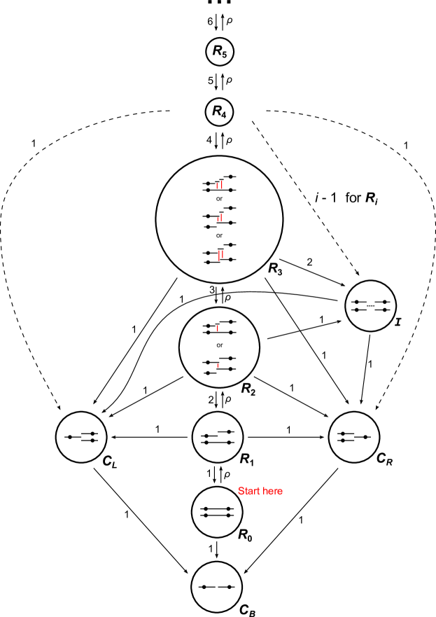
Figure 3: Schematic of the SMC’ back-in-time Markov process for two loci. Dashed arrows show transition rates that apply for all $\boldsymbol{R_{i}}.$ State $\boldsymbol{I}$ is the state in which some portion of the chromosome between the two focal loci has coalesced but neither focal locus has coalesced. The red lines in states $\boldsymbol{R_{2}}$ and $\boldsymbol{R_{3}}$ show the coalescence events that take the process to state $\boldsymbol{I}$.

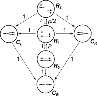
Figure S1: Schematic of the ARG back-in-time Markov process for two loci. The process starts in state $\boldsymbol{R_{0}}$, and transitions to other states occur with the rates indicated by arrows between states.

For comparison, an analogous two-locus continuous-time Markov chain for the ARG is presented in Figure S1. An equivalent process was studied by Simonsen and Churchill (1997) and others. In this model, state $\boldsymbol{R_{1}}$ is reached when the first event is a recombination event, and state $\boldsymbol{R_{2}}$ is reached only after a subsequent recombination event occurs on the ancestral lineage that did not experience the first recombination event, making all ancestral copies of the two loci unlinked.

2.2 Joint probability density functions

Considering the SMC’ model above, let $R_{0}(t)$ represent the probability that the two-locus ancestral coalescent process is in state $\boldsymbol{R_{0}}$ at time $t$, and let $R^{+}(t)$ represent the probability that the process is in any state $\boldsymbol{R_{i}}$, $i\geq 1$, or state $\boldsymbol{I}$, at time $t$. The joint density of coalescence times at the two focal loci is then

$$f_{T_{1},T_{2}}(t_{1},t_{2})=\begin{cases}R_{0}(t_{1})&t_{1}=t_{2}\\ R^{+}(t_{1})e^{-(t_{2}-t_{1})}&t_{1}<t_{2}\\ R^{+}(t_{2})e^{-(t_{1}-t_{2})}&t_{1}>t_{2},\end{cases}$$ (2)

since $R_{0}(t)$ is the rate of entering state $\boldsymbol{C_{B}}$ at time $t$, and $R^{+}(t)$ is the rate of entering either $\boldsymbol{C_{L}}$ or $\boldsymbol{C_{R}}$ at time $t$. The joint density for the ARG and SMC is analogously defined, with $R^{+}(t)$ representing $\boldsymbol{R_{1}}$ and $\boldsymbol{R_{2}}$ under the ARG and $\boldsymbol{R_{1}}$ under the SMC. For the ARG and the SMC, the number of states is finite and $R_{0}(t)$ and $R^{+}(t)$ can be solved using matrix exponentiation. For the SMC’, there is an infinite number of states, representing the possibility of an infinite number of recombination events occurring between the two focal loci. In the Appendix, we derive closed-form expressions for $R_{0}(t)$, $R^{+}(t)$, and $f_{T_{1},T_{2}}(t_{1},t_{2})$. The main idea in these derivations is to recognize the structure of the SMC’ in Figure 3 as a birth-death process with killing. In this formulation the states are $\boldsymbol{R_{i}},\{i\geq 0\}$, a birth corresponds to a recombination event (and the birth rate is constant), a death corresponds to a coalescence event (and the death rate is linear), and killing corresponds to leaving the $\boldsymbol{R_{i}}$ states.

Figure 4 compares the joint coalescence time distributions under the SMC and SMC’, displaying the differences of these joint distributions with the joint distribution of the ARG. The SMC’ provides a much better fit to the ARG for the range of recombination rates compared. Both the SMC and the SMC’ underestimate the density of outcomes where $T_{1}=T_{2}$, but this underestimation is substantially less under the SMC’.

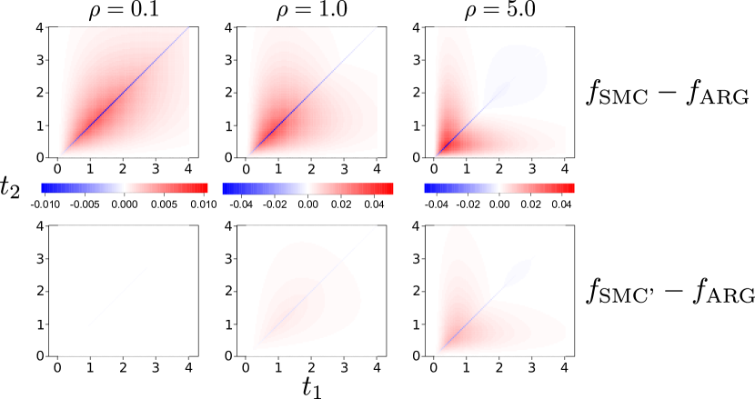
Figure 4: Comparison of the difference in the joint density of coalescence times $f_{T_{1},T_{2}}(t_{1},t_{2})$ between the SMC and ARG (top row) and SMC’ and ARG (bottom row). Comparisons are made for three different recombination rates ($\rho=0.1,1.0,5.0$).

To summarize the difference between the joint distributions more succinctly, we calculated the total variation distance between the SMC and ARG and between the SMC’ and ARG across a range of recombination rates. The total variation distance between the SMC and the ARG is defined as

$$TV\left(\textrm{SMC},\textrm{ARG}\right)=\frac{1}{2}\int_{0}^{\infty}\int_{0}^{\infty}\left|f^{\textrm{SMC}}(t_{1},t_{2})-f^{\textrm{ARG}}(t_{1},t_{2}))\right|dt_{2}dt_{1},$$ (3)

where $f^{\textrm{SMC}}(t_{1},t_{2})$ and $f^{\textrm{ARG}}(t_{1},t_{2})$ are the joint densities $f_{T_{1},T_{2}}(t_{1},t_{2})$ defined under the SMC and ARG, respectively. The total variation distance between the SMC’ and ARG is similarly defined. Figure 5 shows the total variation distance from the ARG for the SMC and SMC’ over a range of recombination rates. Total variation distances were calculated numerically. For both the SMC and SMC’, the total variation distance was maximized at some intermediate recombination rate, approximately $\rho=1.1$ for the SMC and $\rho=3.2$ for the SMC’.

Figure 5: Total variation distance between the SMC and ARG (solid line) and the SMC’ and ARG (dashed line) as a function of recombination rate. Total variation distances were calculated numerically.

2.3 Conditional distribution of coalescence times

In this section we consider the distribution of coalescence times at one locus given the coalescence time at the other. The conditional density of $T_{2}$ given $T_{1}$, $f_{T_{2}|T_{1}}(t_{2}|t_{1})$, can be calculated by dividing the joint density by the marginal distribution of coalescence times at the left locus:

$$f_{T_{2}|T_{1}}(t_{2}|t_{1})=\frac{f_{T_{1},T_{2}}(t_{1},t_{2})}{e^{-t_{1}}}.$$ (4)

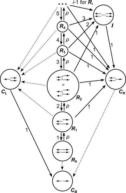
Figure S2: Back-in-time Markov process for generating a coalescence time $T_{2}$ at the right locus conditional on the time $T_{1}=t_{1}$ at the left locus under the SMC’. Starting at time zero in state $\boldsymbol{R_{0}}$, the process follows the transitions indicated by the solid arrows at the rates accompanying these arrows. Transitions indicated by dotted arrows are followed instantaneously at time $t_{1}$. See Hobolth and Jensen (2014) for analogous processes for the ARG and SMC models.

Hobolth and Jensen (2014) introduced a framework for modeling the distribution of $T_{2}$ given $T_{1}$ using a time-inhomogeneous continuous-time Markov chain. (Note that the model called SMC’ in Hobolth and Jensen (2014) is an SMC’-like model of two loci that is not based on the continuous-chromosome SMC’. It is different from the SMC’ model we consider here.) This framework can be extended to the SMC’, producing the continuous-time Markov chain shown in Figure S2. Figure 6 compares the conditional density $f_{T_{2}|T_{1}}(t_{2}|t_{1})$ of coalescence times $t_{2}$ at the right locus conditioned upon the coalescence times $t_{1}$ at the left locus for different values of $t_{1}$ and $\rho$.

We note that recently it was proposed that the mutation rate could be estimated by simulation-based calibration of the increase in mean heterozygosity when moving away from a site of known, low heterozygosity (Lipson et al., 2015). Our expressions for the conditional distribution of coalescence times could provide theoretical expectations for such a statistic.

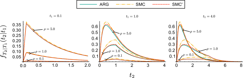
Figure 6: Comparison of densities of coalescence times $t_{2}$ at the right locus conditioned upon coalescence times $t_{1}$ at the left locus. Conditional densities $f_{T_{2}|T_{1}}(t_{2}|t_{1})$ are shown for the ARG, SMC, and SMC’ models for three different rates of recombination between the two loci ($\rho=0.1,1.0,5.0$) and three different conditioned-upon coalescence times $t_{1}$ at the left locus ($t_{1}=0.1,1.0,4.0$). The area under each curve is $P(T_{2}\neq t_{1}|T_{1}=t_{1})$; the conditional probabilities $P(T_{2}=t_{1}|T_{1}=t_{1})$ are not shown.

2.4 Probability of coalescence times being equal to covariance between coalescence times

In the two-locus, back-in-time Markov processes for the SMC, SMC’, and ARG, $T_{1}$ and $T_{2}$ are equal when the state $\boldsymbol{C_{B}}$ is entered through $\boldsymbol{R_{0}}$ rather than $\boldsymbol{C_{L}}$ or $\boldsymbol{C_{R}}$. For the ARG, Simonsen and Churchill (1997) showed that the probability that $T_{1}$ is equal to $T_{2}$ is

$$P_{\textrm{ARG}}(T_{1}=T_{2})=\frac{\rho+18}{\rho^{2}+13\rho+18}.$$ (5)

Under the SMC (McVean and Cardin, 2005),

$$P_{\textrm{SMC}}(T_{1}=T_{2})=\frac{1}{1+\rho}.$$ (6)

Eriksson et al. (2009) used the sequential formulation of the SMC’ to show that

$$\begin{split}P_{\textrm{SMC'}}(T_{1}=T_{2})&=\int_{0}^{\infty}e^{-t}e^{-\rho\lambda(t)}dt\\ &=2^{\rho/2}e^{-\rho/4}(-\rho)^{-\frac{1}{2}-\frac{\rho}{4}}\left[\Gamma\left(\frac{2+\rho}{4}\right)-\Gamma\left(\frac{2+\rho}{4},-\frac{\rho}{4}\right)\right],\end{split}$$ (7)

where ${\lambda(t)=\frac{1}{4}\left(1-e^{-2t}+2t\right)}$ is the exponential rate of encountering a change in coalescence time when the local coalescence time is $t$ and $\Gamma(a,b)=\int_{b}^{\infty}x^{a-1}e^{-x}dx$ is the incomplete gamma function.

For the ARG and SMC, the covariance $\operatorname{Cov}[T_{1},T_{2}]$ is equal to $P(T_{1}=T_{2})$. Eriksson et al. (2009) showed by simulation that this is also true of the SMC’. Here we present a short proof that this is the case for any two-locus model of coalescence where the marginal distribution of coalescence times is exponential with rate $1$.

The expectation $\operatorname{E}[T_{1}T_{2}]$ can be derived using the fact that ${(a-b)^{2}=a^{2}+b^{2}-2ab}$:

$$\begin{split}2\operatorname{E}[T_{1}T_{2}]&=\operatorname{E}[T_{1}^{2}]+\operatorname{E}[T_{2}^{2}]-\operatorname{E}[(T_{1}-T_{2})^{2}]\\ &=2+2-\operatorname{E}\big{[}(T_{1}-T_{2})^{2}|T_{1}\neq T_{2}\big{]}P(T_{1}\neq T_{2})\\ &=4-2P(T_{1}\neq T_{2}).\end{split}$$ (8)

The final equality in (8) follows from the fact that $|T_{1}-T_{2}|$ has an Exponential distribution with rate $1$ when $T_{1}\neq T_{2}$. Therefore $\operatorname{E}[T_{1}T_{2}]=2-P(T_{1}\neq T_{2})$ and

$$\begin{split}\operatorname{Cov}[T_{1},T_{2}]&=\operatorname{E}[T_{1}T_{2}]-\operatorname{E}[T_{1}]\operatorname{E}[T_{2}]\\ &=\operatorname{E}[T_{1}T_{2}]-1\\ &=P(T_{1}=T_{2}).\end{split}$$ (9)

This result holds in other situations with exponential coalescence times, for example in the context of the population-divergence model considered by Eriksson et al. (2009) (in which case the marginal distribution is exponential plus a constant) and for the various covariances used by McVean (2002) to calculate $\sigma_{d}^{2}$, the approximation to the linkage disequilibrium measure $r^{2}$.

It is interesting to consider $\operatorname{Cov}[T_{1},T_{2}]=P(T_{1}=T_{2})$ when $\rho$ is small. For the ARG, consideration of (5) shows that ${\operatorname{Cov}[T_{1},T_{2}]=P_{\textrm{ARG}}(T_{1}=T_{2})=1-2\rho/3+O(\rho^{2})}$. Likewise, for the SMC, (6) shows that ${\operatorname{Cov}[T_{1},T_{2}]=P_{\textrm{SMC}}(T_{1}=T_{2})=1-\rho+O(\rho^{2})}$. For the SMC’, the integral representation of $P_{\textrm{SMC'}}(T_{1}=T_{2})$ in (7) allows for the calculation of this quantity as a first-order expansion in $\rho$:

$$\begin{split}\operatorname{Cov}[T_{1},T_{2}]=P_{\textrm{SMC'}}(T_{1}=T_{2})&=\int_{0}^{\infty}e^{-t}e^{-\rho\lambda(t)}dt\\ &=1-\rho\int_{0}^{\infty}e^{-t}\lambda(t)dt+O(\rho^{2})=1-\frac{2\rho}{3}+O(\rho^{2}).\end{split}$$ (10)

Thus, $\operatorname{Cov}[T_{1},T_{2}]$ (or $P(T_{1}=T_{2})$) is the same up to order $\rho^{2}$ under the ARG and SMC’.

2.5 Coalescence times at recombination sites

In this section, we show that the joint distribution of coalescence times on either side of a recombination event is the same under the SMC’ and marginally under the ARG, and we derive this distribution. Consider the continuous-time Markov chains representing the two-locus SMC’ and ARG models (Figures 3 and S1, respectively) in the limit of $\rho\to 0$ and conditioning on the first event being a recombination event. These processes represent the joint distribution of coalescence times on either side of a recombination event under the ARG and SMC’. In both of these processes, the waiting time until the first event, conditional on that event being a recombination event, has an exponential distribution with rate $1+\rho$, which converges to $1$ as $\rho\to 0$. After that first recombination event, the rate of all additional recombination events converges to zero in the $\rho\to 0$ limit, so all of the remaining events must be coalescence events, each of which occurs with rate $1$. Under the ARG and the SMC’, the coalescence events that are possible from state $\boldsymbol{R_{1}}$ are the same. Thus, the joint distribution of coalescence times at recombination sites is the same under the SMC’ and the ARG.

Figure 7A shows the two-locus continuous-time Markov chain representing this conditional process. This Markov chain starts in a special initial state $\boldsymbol{R_{0}^{*}}$, out of which the first event is always a recombination event, which happens with rate $1$, as described above. In previous sections, we used $T_{1}$ and $T_{2}$ to represent the coalescence times at two loci some fixed distance apart. To avoid confusion, in this section we use $S$ and $T$ to represent the coalescence times on the left and right sides of a recombination event, respectively.

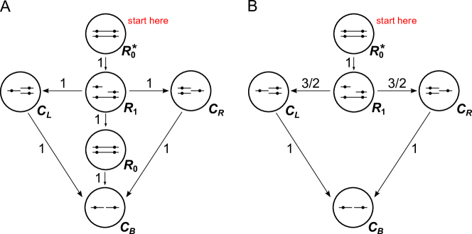
Figure 7: Two-locus continuous-time Markov chains representing the ARG and SMC’ models in the $\rho\to 0$ limit, conditional on the first event being a recombination event. These processes represent the joint distribution of coalescence times on either side of a recombination site under the ARG and SMC’. The state $\boldsymbol{R_{0}^{*}}$ is a special starting state out of which the first event is always a recombination event. Panel A shows the process unconditional on whether $S=T$, and Panel B shows the process conditional on $S\neq T$. The model representing the joint distribution of coalescence times at recombination sites under the SMC is equivalent to the model in Panel B with the transition rates from $\boldsymbol{R_{1}}$ to $\boldsymbol{C_{L}}$ and $\boldsymbol{C_{R}}$ equal to $1$ instead of $3/2$.

Recombination events are visible in sequence data only if they change the local coalescence time. Thus, it is of special interest to condition on $S\neq T$ in the above model in order to derive the joint distribution of coalescence times on either side of a change in coalescence times under the ARG and SMC’. Conditioning on $S\neq T$, the transition out of $\boldsymbol{R_{1}}$ must be into either $\boldsymbol{C_{L}}$ or $\boldsymbol{C_{R}}$. These transitions occur with conditional rate $3/2$, since the total rate of leaving $\boldsymbol{R_{1}}$ is three in the unconditional model, and two of the ways of leaving $\boldsymbol{R_{1}}$ result in the coalescence times being different.

The continuous-time Markov chain representing coalescence times on either side of a change in coalescence times (i.e., at recombination sites where $S\neq T$) is shown in Figure 7B. Under this model, the joint distribution of $S$ and $T$ is that of

$$(S,T)\sim\big{(}X_{1}+X_{2}+RX_{3},\ X_{1}+X_{2}+(1-R)X_{3}\big{)},$$ (11)

where $X_{1}\sim\operatorname{Exp}(1)$, $X_{2}\sim\operatorname{Exp}(3)$, $R\sim\operatorname{Bernoulli}(1/2)$, $X_{3}\sim\operatorname{Exp}(1)$, and the random variables are independently distributed.

Under the SMC, the continuous-time Markov chain representing the joint distribution of coalescence times at recombination sites is equivalent to the model in Figure 7B with the transition rates from $\boldsymbol{R_{1}}$ to $\boldsymbol{C_{L}}$ and $\boldsymbol{C_{R}}$ equal to $1$ instead of $3/2$. Under this model for the SMC, the joint distribution of coalescence times on either side of a recombination event is that of

$$(S,T)\sim(X_{1}+X_{2},X_{1}+X_{3}),$$ (12)

where $X_{1}$, $X_{2}$, and $X_{3}$ are all mutually independent exponential random variables with rate $1$.

In the Supporting Information, we use these Markov processes to derive the joint, marginal, and conditional distributions of coalescence times at recombination sites under the ARG, SMC’, and SMC. These calculations confirm previous derivations of Carmi et al. (2014) for the SMC’ and Li and Durbin (2011) for the SMC.

2.5.1 SMC’ as the canonical first-order Markov approximation to ARG

Under the sequential formulation of the continuous-chromosome ARG, SMC, and SMC’ models, the infinitesimal probability of a recombination event occurring in the interval $(x,x+dx)$ given the coalescence time $s$ at $x$ is $s\,dx$. This fact, together with the fact that the joint distribution of coalescence times at recombination sites is the same under the ARG and SMC’ (whether or not the coalescence time changes), implies that the conditional distribution of coalescence times at point $x+dx$ given the coalescence time at point $x$ is the same under the SMC’ and ARG.

This fact demonstrates that the pairwise SMC’ is the canonical first-order Markov approximation for the pairwise ARG. Given an infinite-order Markov chain $\{X_{i},i=0,1,2,\dots\}$, where the distribution of each $X_{j}$ depends on all previous $X_{i}$, $i<j$, the canonical $k$-order Markov approximation to $\{X_{i}\}$ is the Markov chain $\{X_{i}^{[k]}\}$ satisfying

$$P(X_{n}^{[k]}|X_{n-1}^{[k]}=x_{n-1},\ldots,X_{n-k}^{[k]}=x_{n-k})=P(X_{n}|X_{n-1}=x_{n-1},\ldots,X_{n-k}=x_{n-k}).$$ (13)

That is, the transition probabilities under the $k$-order canonical Markov approximation are equal to the transition probabilities conditional on the previous $k$ states under the infinite-order chain. See Schwarz (1976), Fernández and Galves (2002), and Gallo et al. (2013) for examples of mathematical studies of canonical Markov approximations of infinite-order Markov chains.

Here we informally extend the terminology of canonical Markov approximations to continuous processes. The SMC’ is the canonical first-order Markov approximation to the ARG because the distribution of coalescence times at $x+dx$ conditional on the coalescence time at $x$ is the same under the ARG (an infinite-order, sequentially non-Markovian continuous process) and the SMC’ (a first-order sequentially Markov continuous process). In this sense, the SMC’ is the most natural first-order sequentially Markov approximation to the ARG.

2.6 Asymptotic bias of the population-size estimators under SMC and SMC’

Given the joint density of pairwise coalescence times at recombination sites under the ARG, it is possible to determine the asymptotic bias of maximum-likelihood population size estimators derived from the pairwise SMC and SMC’ likelihood functions. These likelihood functions give the probability of observing a sequence of pairwise coalescence times and corresponding segment lengths across a chromosome under the SMC and SMC’ models. Related likelihood functions (allowing for variable historical population size) are implicitly maximized in the PSMC and MSMC inference procedures (Li and Durbin, 2011; Schiffels and Durbin, 2014, respectively). These inference procedures are hidden Markov model (HMM) methods in which the local coalescence times (or genealogies) and segment lengths are hidden states inferred from sequence data.

Here, we consider the estimators that would be obtained if the hidden states in these models were actually observable (see also Kim et al., 2015). We are motivated by the fact that any biases of the estimators we investigate are likely to be inherent in the full HMM-based inference procedures, since these biases would be present even with perfect knowledge of an infinite number of coalescence times. Furthermore, by analyzing estimators derived from the hidden coalescence states, we isolate the bias that is due to choice of coalescent algorithm (SMC vs. SMC’) from the bias due to the mutation model or discretization of the continuous hidden states in a full HMM approach to inference.

To investigate the asymptotic properties of these estimators, we assume that data are generated under the ARG, such that at a fixed point the distribution of pairwise coalescence times is exponential with rate equal to $1$ and an ancestral segment of length $l$ recombines back in time at rate $\rho l/2$. Segment lengths are measured in units of the true scaled recombination parameter $\rho$. Data generated under this model can be represented as a sequence of pairwise coalescence times and corresponding segment lengths: $\{(t_{i},l_{i}):1\leq i\leq k\}$.

We are interested in estimating a single relative population size $\eta$ (defined relative to the true population size, $N$). If the data are modeled by the SMC or SMC’, the likelihood of a particular value of $\eta$ is

$$L(\eta|\{(t_{i},l_{i})\})=\frac{1}{\eta}e^{-\frac{t_{1}}{\eta}}\prod_{i=2}^{k}q(t_{i}|t_{i-1};\eta)\prod_{i=1}^{k}\lambda(t_{i};\eta)e^{-\lambda(t_{i};\eta)l_{i}},$$ (14)

where $q(t|s)$ is the transition function and $\lambda(t;\eta)$ is the rate of encountering the end of a segment given $t$, with both quantities pertaining to the sequentially Markov coalescent model being used to calculate the likelihood.

In the Appendix, we show that if the SMC is used, the maximum-likelihood estimate of $\eta$ converges to approximately $0.95$ as the chromosome gets infinitely long. If the SMC’ is used, the estimate is approximately unbiased in the same limit. If the data are reduced to just the segment ages, the likelihood equation is

$$L(\eta|\{(t_{i},l_{i})\})=\frac{1}{\eta}e^{-\frac{t_{1}}{\eta}}\prod_{i=2}^{k}q(t_{i}|t_{i-1};\eta).$$ (15)

Using this reduced likelihood, the asymptotic maximum-likelihood estimate is asymptotically unbiased under the SMC’. Under the SMC, the reduced likelihood and the full likelihood produce the same maximum-likelihood estimate (see Appendix).

We confirm the asymptotic bias of the SMC estimator and the apparent lack of asymptotic bias of the SMC’ estimators by simulation. Figure 8 shows 100 simulated estimates calculated using the SMC, SMC’, and reduced SMC’ likelihood functions. Each estimate was calculated using 100 independent pairs of chromosomes simulated under the ARG, with each chromosome of total length $4Nr=1000$, where $N$ is the diploid size and $r$ is the per-generation probability of recombination. Likelihood functions were multiplied across independent pairs of chromosomes, and the same set of simulations was used to produce the estimates for all three likelihood functions.

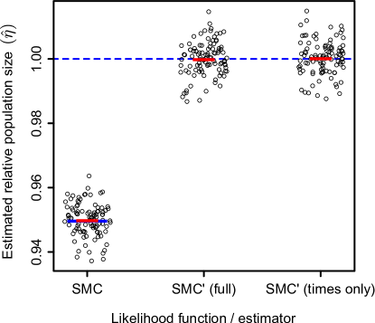
Figure 8: Maximum-likelihood estimates of relative population size with three different Markov chain likelihood functions. For each simulation, the segment lengths and coalescence times were taken from 100 independent pairs of chromosomes, with each chromosome being of length $\rho=4Nr=1000$ simulated under the ARG. A maximum-likelihood estimate was calculated using the SMC, SMC’, and times-only SMC’ likelihood functions (equations (25), (26), and (15), respectively). The true scaled population size is $\eta=1$, shown with the dashed blue line. The predicted asymptotic bias of the SMC likelihood function ($\hat{\eta}\approx 0.95$) is shown with a solid blue line. The sample mean of the estimates calculated with each likelihood function is shown with a solid red line. A total of $100$ simulated datasets were analyzed.

3 Discussion

We have presented a continuous-time Markov chain that describes the pairwise coalescence times at two fixed loci evolving under the SMC’ model of coalescence with recombination. We analyzed this Markov chain to derive the joint distribution of coalescence times at the two loci and the conditional distribution of coalescence times at one locus given the coalescence time at the other. We compared these distributions to those of the ARG and SMC models and found that the difference between the ARG and the SMC’ was much less than the difference between the ARG and the SMC.

We showed that the conditional distribution of coalescence times at point $x+dx$ given the coalescence time at $x$ is the same under the ARG and SMC’. This implies that the SMC’ is the canonical first-order approximation to the pairwise ARG. However, this correspondence is true only of the continuous-chromosome models. If instead the ARG is a model of the genealogies at a sequence of discrete loci, then the first-order canonical Markov approximation is the Markov approximation obtained by modeling a conditional ARG between every successive pair of loci. This model was studied by Hobolth and Jensen (2014), who referred to the model as a “natural” Markov approximation to the ARG. Conceptually similar sequentially Markov coalescent models have been used in the so-called “coalescent hidden Markov model” family of methods (Hobolth et al., 2007; Dutheil et al., 2009; Mailund et al., 2011).

Chen et al. (2009) presented a method of simulating data under higher-order sequentially Markov approximations to the ARG, where the ARG of some number of preceding loci is retained in the process of generating the marginal genealogy at a given locus. They showed by simulation that higher-order approximations generate times until most recent common ancestry that are more consistent with the ARG than do lower-order approximations, but little theoretical work on these higher-order Markov approximations has been done.

The two-locus Markov chains analyzed in this paper assume a single well-mixed population, but natural populations often have more complex demographic histories, featuring, for example, variable historical population sizes, migration between subpopulations, and/or past divergence from other populations. The theoretical properties of the sequential, across-the-chromosome formulations of the pairwise SMC and SMC’ with variable population sizes have been studied previously (Li and Durbin, 2011; Schiffels and Durbin, 2014). Eriksson et al. (2009) used simulation to study two-locus properties of the SMC’ with population bottlenecks, migration between subpopulations, and divergence between populations. They found that the SMC’ generally performs well in these contexts. The two-locus Markov chains we study here could be extended to include these features (as was done for the ARG by Lessard and Wakeley (2003) and Eriksson and Mehlig (2004)), which would provide a framework for calculating exact quantities for the two-locus SMC and SMC’ in the context of structured populations. We leave this for future work.

We calculated the asymptotic bias of a population size estimator under the pairwise SMC to be approximately 95% of the true population size. This is not a very large bias, but given the continued use of the SMC model in population-genomic inference methods (Palamara et al., 2012; Sheehan et al., 2013; Rasmussen et al., 2014), there is an apparent need to re-examine the consequences of using the simpler SMC model instead of the slightly more complicated SMC’ model. For example, it will be important to consider whether including the possibility of varying population sizes will increase or decrease asymptotic bias. In this context, using the SMC as a basis for a likelihood function may also bias the estimates of the magnitude and timing of population size changes, since the longer segments produced by the ARG will seem younger when they are modeled under the SMC.

Depending on the particular application, it may sometimes be mathematically difficult to employ the SMC’ instead of the SMC. Nevertheless, the SMC’ is the model underlying two recently introduced population-genetic inference methods: the multiple SMC (MSMC) method of Schiffels and Durbin (2014) (which simplifies to a PSMC’ inference procedure when the number of haplotypes is two) and a procedure based on the distribution of distances between heterozygous bases, introduced by Harris and Nielsen (2013). In each case it was acknowledged that the SMC’ provided more accurate results than the SMC.

From the arguments that led to the development of the continuous-time Markov chains representing the joint distribution of coalescence times at recombination sites (Figure 7), it seems that the joint distribution of coalescence times on either side of a recombination event will be the same under a variety of demographic scenarios. If one were to allow variable population historical size, the waiting time until the conditioned-upon recombination event would still be the same under the SMC’ and ARG, and the remaining coalescence events would also be distributed identically. Likewise, when there is population substructure with migration between subpopulations, the distribution of events occurring at recombination sites should be the same under the SMC’ and ARG. Finally, when there are more than two haplotypes sampled, it seems that the joint distributions of genealogies on either side of a recombination event would be the same between the SMC’ and the ARG marginally. These ideas need to be properly explored in future studies, but they suggest that asymptotic bias due to using the SMC’ in place of the ARG will be minimal under a variety of demographic scenarios.

4 Acknowledgments

We thank Erik van Doorn and Søren Asmussen for identifying the correspondence to birth-death models with killing (see Appendix). We are grateful to John Wakeley and Paul Marjoram, and two anonymous reviewers for comments that helped improve this article. S.C. thanks the Human Frontier Science Program for financial support.

5 References

6 Appendix

6.1 Derivation of joint density of pairwise coalescence times at two loci

To calculate the joint density of coalescence times, it is necessary to calculate $R_{j}(t)$, the probability that the SMC’ two-locus Markov process (Figure 3) is in state $\boldsymbol{R_{j}}$ at time $t$, and $I(t)$, the probability that the SMC’ process is in state $\boldsymbol{I}$ at time $t$. To solve for $R_{j}(t)$, one can use the forward Kolmogorov equation (for $j\geq 1$)

$$R_{j}^{\prime}(t)=\rho R_{j-1}(t)+(j+1)R_{j+1}(t)-(2j+1+\rho)R_{j}(t).$$ (16)

Through substitution, the solution to (16) can be shown to be

$$R_{j}(t)=R_{0}(t)\frac{\left[\frac{\rho}{2}(1-e^{-2t})\right]^{j}}{j!}.$$ (17)

To find $R_{0}(t)$, we note that it is equal to $f_{T_{1},T_{2}}(t,t)$ (see Eq. (2)). In turn, ${f_{T_{1},T_{2}}(t,t)=f_{T_{1}}(t)P(T_{2}=t|T_{1}=t)}$, where $f_{T_{1}}(t)=e^{-t}$ is the marginal distribution of coalescence times at the first (or second) locus and ${P(T_{2}=t|T_{1}=t)=e^{-\rho\lambda(t)}}$ is the probability of no change in coalescence times given the coalescence time $t$ at the first locus. Here $\lambda(t)=\frac{1}{4}\left(1-e^{-2t}+2t\right)$ is the exponential rate of encountering a change in coalescence time along the chromosome given that the local coalescence time is $t$ (Eriksson et al., 2009; Carmi et al., 2014). Thus $R_{0}(t)$ is given by

$$R_{0}(t)=e^{-t}e^{-\rho\lambda(t)}.$$ (18)

This completes the solution of $R_{j}(t)$. Using Figure 3,

$$R^{+}(t)=I(t)+\sum_{j=1}^{\infty}R_{j}(t),$$ (19)

where $I(t)$ is the probability that the process is in state $\boldsymbol{I}$ at time $t$. Using (17) and (18) we get

$$\begin{split}\sum_{j=1}^{\infty}R_{j}(t)&=R_{0}(t)\sum_{j=1}^{\infty}\frac{\left[\frac{\rho}{2}(1-e^{-2t})\right]^{j}}{j!}\\ &=e^{-t}e^{-\frac{\rho}{4}(1+2t-e^{-2t})}\left[e^{\frac{\rho}{2}\left(1-e^{-2t}\right)}-1\right].\end{split}$$ (20)

Next, $I(t)$ satisfies the forward Kolmogorov equation

$$I^{\prime}(t)=\sum_{j=2}^{\infty}(j-1)R_{j}(t)-2I(t),$$ (21)

the solution to which is

$$\begin{split}I(t)&=e^{-2t}\int_{0}^{t}e^{2u}\sum_{j=2}^{\infty}(j-1)R_{j}(u)du\\ &=e^{-2t}\int_{0}^{t}R_{0}(u)\left\{2e^{2u}+e^{\frac{\rho}{2}\left(1-e^{-2u}\right)}\left[(\rho-2)e^{2u}-\rho\right]\right\}du\\ &=e^{-2t}\bigg{\{}1-e^{\frac{1}{4}\left(-2t(\rho-2)+\rho-e^{-2t}\rho\right)}\\ &\hskip 28.45274pt-e^{-\frac{\rho}{4}}2^{\frac{\rho-4}{2}}(-\rho)^{-\frac{\rho-2}{4}}\left[\Gamma\left(\frac{\rho-2}{4},-\frac{\rho}{4}\right)-\Gamma\left(\frac{\rho-2}{4},-\frac{e^{-2t}\rho}{4}\right)\right]\bigg{\}}.\end{split}$$ (22)

Here, $\Gamma(a,b)=\int_{b}^{\infty}x^{a-1}e^{-x}dx$ is the incomplete gamma function.

Together (18), (19), (20), and (22) give the joint distribution (2) for the SMC’. For the ARG and SMC, the quantities analogous to $R_{0}(t)$ and $R^{+}(t)$ for these models can be obtained by exponentiating the rate matrices implicit in Figures 2 and S1. For the SMC, the joint distribution can also be derived using the representation (1).

The walk on the states $\boldsymbol{R_{0}},\boldsymbol{R_{1}},\boldsymbol{R_{2}},\dots$ constitutes a birth-death process with killing, where birth events correspond to additional recombination events taking the process from $\boldsymbol{R_{i}}$ to $\boldsymbol{R_{i+1}}$, death events correspond to coalescence events that take the process from $\boldsymbol{R_{i}}$ to $\boldsymbol{R_{i-1}}$, and killing events, which take the process to an absorbing state, here correspond to coalescence events that take the process to $\boldsymbol{C_{L}}$, $\boldsymbol{C_{R}}$, or $\boldsymbol{I}$. Under this formulation, the birth rate is constant $\lambda_{i}=\rho$, the death rate is linear $\mu_{i}=i$, and the killing rate is linear $\gamma_{i}=i+1$. This class of processes was studied by van Doorn and Zeifman (2005), who demonstrated a different approach for calculating $R_{i}(t)$. This alternative approach (not shown) confirms our derivation of (18).

6.2 Calculating asymptotic bias

We are interested in estimating a single relative population size $\eta$ (defined relative to the true population size, $N$), which must be incorporated into the transition density function $q(t|s)$ at recombination sites under the SMC and SMC’. Under the SMC, this transition density function is

$$q_{\textrm{SMC}}(t|s;\eta)=\begin{cases}\frac{1}{s}(1-e^{-t/\eta})&t<s\\[10.00002pt] \frac{1}{s}e^{-(t-s)/\eta}(1-e^{-s/\eta})&t>s.\end{cases}$$ (23)

This is equivalent to the conditional density (S6) with the addition of a relative population size parameter. Under the SMC’, the transition function is

$$q_{{\rm SMC^{\prime}}}(t|s;\eta)=\begin{cases}\frac{\frac{2}{\eta}\left(1-e^{-2t/\eta}\right)}{1+\frac{2s}{\eta}-e^{-2s}}&t<s\\[10.00002pt] \frac{\frac{2}{\eta}e^{-(t-s)/\eta}\left(1-e^{-2s/\eta}\right)}{1+\frac{2s}{\eta}-e^{-2s}}&t<s,\end{cases}$$ (24)

which is equivalent to the conditional density (S3) with a relative population size parameter included.

Under the SMC, given the local coalescence time $t$, the distance along the chromosome until the nearest recombination event (measured in units of $\rho$) is exponentially distributed with rate $t$ (McVean and Cardin, 2005). The likelihood function for a single relative population size $\eta$ under the SMC is thus

$$\begin{split}L_{{\rm SMC}}(\eta|\{(t_{i},l_{i})\})&=\frac{1}{\eta}e^{-\frac{t_{1}}{\eta}}\prod_{i=2}^{k}q_{{\rm SMC}}(t_{i}|t_{i-1};\eta)\prod_{i=1}^{k}t_{i}e^{-t_{i}l_{i}}\\ &\propto\frac{1}{\eta}e^{-\frac{t_{1}}{\eta}}\prod_{i=2}^{k}q_{{\rm SMC}}(t_{i}|t_{i-1};\eta).\end{split}$$ (25)

Under the SMC’, the likelihood function for a relative population size $\eta$ is

$$L_{{\rm SMC^{\prime}}}(\eta|\{(t_{i},l_{i})\})=\frac{1}{\eta}e^{-\frac{t_{1}}{\eta}}\prod_{i=2}^{k}q_{{\rm SMC^{\prime}}}(t_{i}|t_{i-1};\eta)\prod_{i=1}^{k}\lambda(t_{i},\eta)e^{-\lambda(t_{i},\eta)l_{i}},$$ (26)

where $\lambda(t,\eta)=\frac{1}{4}\left[\eta(1-e^{-2t/\eta})+2t\right]$ is the exponential rate of encountering recombination events that change the coalescence time when the local coalescence time is $t$ (Eriksson et al., 2009). Note that under the SMC, the length $l_{i}$ of a segment is independent of the relative population size $\eta$ given the local coalescence time $t_{i}$. This is not true for the SMC’, since the probability that the coalescence time changes at a recombination site depends on the population size.

As the length of the chromosome increases and the number of coalescence-time changes goes to infinity, the asymptotic maximum-likelihood estimate $\hat{\eta}^{*}$ of the relative population size under the SMC is

$$\begin{split}\hat{\eta}^{*}&=\lim_{k\to\infty}\operatorname*{\arg\!\max}_{\eta}\ \frac{1}{\eta}e^{-\frac{t_{1}}{\eta}}\prod_{i=2}^{k}q_{{\rm SMC}}(t_{i}|t_{i-1};\eta)\\ &=\lim_{k\to\infty}\operatorname*{\arg\!\max}_{\eta}\ \left\{\log\left(\frac{1}{\eta}e^{-\frac{t_{1}}{\eta}}\right)+\sum_{i=2}^{k}\log\left[q_{{\rm SMC}}(t_{i}|t_{i-1};\eta)\right]\right\}\\ &=\lim_{k\to\infty}\operatorname*{\arg\!\max}_{\eta}\ \sum_{i=2}^{k}\log\left[q_{{\rm SMC}}(t_{i}|t_{i-1};\eta)\right]\\ &=\operatorname*{\arg\!\max}_{\eta}\ \operatorname{E}_{{\rm ARG}}\big{[}\log(q_{{\rm SMC}}(T|S;\eta))\big{]}\\ &=\operatorname*{\arg\!\max}_{\eta}\ \int_{0}^{\infty}\int_{0}^{\infty}\pi_{{\rm SMC^{\prime}}}(s)q_{{\rm SMC^{\prime}}}(t|s;1)\log\left(q_{{\rm SMC}}(t|s;\eta)\right)dtds\\ &\approx 0.95.\end{split}$$ (27)

Here the penultimate equality holds only if there is ergodic (i.e., law-of-large-numbers-like) convergence of the sequence of pairs of coalescence times on either side of a recombination site under the ARG. In the Supporting Information, we show that the continuous-chromosome pairwise ARG is ergodic. That is, the mean coalescence time across a long chromosome converges to the mean coalescence time at a single point along the chromosome. We are unable to prove the ergodicity of the sequence of pairs of coalescence times at recombination sites where the coalescence time changes; instead, we note that (27) is supported by simulation (see above). We also note that Wiuf (2006) proved the ergodicity of the discrete-locus ARG under a variety of neutral demographic models. A similarly in-depth proof may also apply for continuous-chromosome models, but we do not explore the point further.

In (27), the ultimate equality follows from the fact that the joint distribution of coalescence times is marginally the same at recombination sites under the ARG and the SMC’. Numerical maximization of the double integral shows that the maximum-likelihood estimate of a single population size $N$ under the pairwise SMC is asymptotically biased, with the asymptotic estimate being approximately $0.95N$.

Under the ARG, the stationary distribution of lengths between recombination events that change the local coalescence time (i.e., the identity-by-descent segment length distribution) is slightly different from that of the SMC’. (They are different because subsequent recombination events “heal” with slightly different probabilities under the ARG, while under the SMC’, each subsequent recombination event “heals” with the same probability.) Under the ARG, the identity-by-descent (IBD) length distribution is not currently known. Given that under the SMC’ the maximum-likelihood estimator for a relative population size involves the observed lengths, it is not currently possible to calculate the asymptotic bias of the pairwise SMC’ maximum-likelihood estimator of a single population size. However, the IBD length distribution under the ARG is approximated very closely by the SMC’ IBD length distribution (Carmi et al., 2014), so the SMC’ estimator is likely to be nearly asymptotically unbiased.

1 Supporting Information

1.1 Coalescence time distributions at recombination sites

Here, we derive the joint, marginal (i.e., one-locus), and conditional distributions of coalescence times at recombination sites where the coalescence time changes under the ARG, SMC’, and SMC. The distributions related to the ARG and SMC’ are derived from analysis of the continuous-time Markov chains representing coalescence times at such recombination sites under these models (Figure 7). Under the ARG and SMC’, the joint density function of coalescence times at recombination sites that change the coalescence time (i.e., the joint density of $S$ and $T$) is

$$f_{S,T}(s,t)=\begin{cases}\frac{3}{4}\left(1-e^{-2s}\right)e^{-t}&s<t\\[7.5pt] \frac{3}{4}\left(1-e^{-2t}\right)e^{-s}&s>t,\end{cases}$$ (S1)

and the marginal density function of $S$ (or $T$) is

$$\pi(s)=\frac{3}{8}e^{-s}\left(2s+1-e^{-2s}\right).$$ (S2)

The conditional distribution of $T$ given $S$ is

$$f_{T|S}(t|s)=\frac{f_{S,T}(s,t)}{\pi(s)}=\begin{cases}\frac{2\left(1-e^{-2t}\right)}{1-e^{-2s}+2s}&t<s\\[7.5pt] \frac{2e^{-(t-s)}\left(1-e^{-2s}\right)}{1-e^{-2s}+2s}&t>s.\end{cases}$$ (S3)

Equations (S1), (S2), and (S3) hold marginally at recombination sites where the coalescence time changes under both the ARG and SMC’. Equations (S2) and (S3) were derived for the SMC’ by Carmi et al. (2014, see eqns. (8) and (9), respectively), confirming our derivation.

Under the SMC the process for generating coalescence times at recombination sites is equivalent to the continuous-time Markov chain in Figure 7B with the transition rates from $\boldsymbol{R_{1}}$ to $\boldsymbol{C_{L}}$ and $\boldsymbol{C_{R}}$ equal to $1$ instead of $3/2$. Under this model for the SMC, the joint density of coalescence times on either side of a recombination event is

$$f_{S,T}(s,t)=\begin{cases}e^{-t}(1-e^{-s})&s<t\\[7.5pt] e^{-s}(1-e^{-t})&s>t\end{cases}$$ (S4)

and the marginal density of $S$ (or $T$) is

$$\pi(s)=se^{-s}.$$ (S5)

The conditional distribution of $T$ given $S$ under the SMC is

$$f_{T|S}(t|s)=\frac{f_{S,T}(s,t)}{\pi(s)}=\begin{cases}\frac{1-e^{-t}}{s}&t<s\\ \frac{e^{-(t-s)}(1-e^{-s})}{s}&t>s,\end{cases}$$ (S6)

which confirms the derivation of Li and Durbin (2011, cf. their Eq. (S6)).

1.2 Pairwise ARG is ergodic

Here we show that the pairwise ARG is sequentially ergodic. Let $\{t(x)\}_{x\geq 0}$ represent the random pairwise coalescence time at point $x$ along two aligned, continuous, infinitely-long chromosomes modeled by the ARG. Let time be scaled such that the marginal distribution of $t(x)$ is exponential with rate $1$ for all $x\geq 0$, and thus $\operatorname{E}[t(x)]=1$. Let the distance across the chromosome be measured such that a segment of length $l$ recombines apart back in time at rate $l/2$. (Equivalently, a recombination event happens in the chromosome interval $(x,x+dx)$ in the time interval $(t,t+dt)$ with infinitesimal probability $dx\,dt$.)

One useful property of $t(x)$ is that it is strongly stationary. That is, the joint distribution of $\{t(x)\}_{a\leq x\leq b}$ is the same as the joint distribution of $\{t(x)\}_{a+h\leq x\leq b+h}$ for all $0\leq a<b$ and $h>0$. To see that this is the case, consider the Wiuf and Hein (1999) algorithm for constructing an ARG sequentially across the chromosome: at a given point, a genealogy is drawn from the marginal distribution of genealogies, and then the algorithm proceeds along the chromosome generating recombination events and genealogies, where at each point along the chromosome, such events are drawn from the conditional distribution given all previous coalescence and recombination events. The initial point from which the marginal genealogy is drawn has no effect on the resulting joint distribution of genealogies.

A stationary process $t(x)$ is ergodic if the covariance function $r(x)$ converges to zero as $x$ goes to infinity (Karlin and Taylor, 1975). Under the ARG, the covariance function is

$$r(x)=\frac{x+18}{x^{2}+13x+18},$$ (S7)

which satisfies this condition. Thus the pairwise ARG is sequentially ergodic: the mean coalescence time across a long chromosome converges to the mean coalescence time at a single point. A similar proof could be given for the discrete-locus ARG with evenly spaced loci, which has a covariance function of the same form as the continuous-chromosome ARG.

1.3 Supplementary Figures

References

- Carmi et al. (2014) Carmi, S., P. R. Wilton, J. Wakeley, and I. Pe’er, 2014 A renewal theory approach to IBD sharing. Theoretical Population Biology 97: 35–48.
- Chen et al. (2009) Chen, G. K., P. Marjoram, and J. D. Wall, 2009 Fast and flexible simulation of DNA sequence data. Genome Research 19: 136–142.
- Dutheil et al. (2009) Dutheil, J. Y., G. Ganapathy, A. Hobolth, T. Mailund, M. K. Uyenoyama, et al., 2009 Ancestral population genomics: The coalescent hidden Markov model approach. Genetics 183: 259–274.
- Eriksson et al. (2009) Eriksson, A., B. Mahjani, and B. Mehlig, 2009 Sequential Markov coalescent algorithms for population models with demographic structure. Theoretical Population Biology 76: 84–91.
- Eriksson and Mehlig (2004) Eriksson, A., and B. Mehlig, 2004 Gene-history correlation and population structure. Physical Biology 1: 220.
- Fernández and Galves (2002) Fernández, R., and A. Galves, 2002 Markov approximations of chains of infinite order. Bulletin of the Brazilian Mathematical Society 33: 1–12.
- Gallo et al. (2013) Gallo, S., M. Lerasle, and D. Takahashi, 2013 Markov approximation of chains of infinite order in the -metric. Markov Processes and Related Fields 19: 51–82.
- Griffiths and Marjoram (1997) Griffiths, R., and P. Marjoram, 1997 An ancestral recombination graph. In P. Donnelly and S. Tavaré, editors, Progress in Population Genetics and Human Evolution, volume 87 of IMA Volumes in Mathematics and Its Application. Springer-Verlag, New York, 257–270.
- Harris and Nielsen (2013) Harris, K., and R. Nielsen, 2013 Inferring demographic history from a spectrum of shared haplotype lengths. PLoS Genetics 9: e1003521.
- Hobolth et al. (2007) Hobolth, A., O. F. Christensen, T. Mailund, and M. H. Schierup, 2007 Genomic relationships and speciation times of human, chimpanzee, and gorilla inferred from a coalescent hidden Markov model. PLoS Genetics 3: e7.