A Comparative Analysis of the Supernova Legacy Survey
Sample with $\Lambda$CDM and the $R_{\rm h}=ct$ Universe⁷

Abstract

The use of Type Ia SNe has thus far produced the most reliable measurement of the expansion history of the Universe, suggesting that $\Lambda$CDM offers the best explanation for the redshift–luminosity distribution observed in these events. But the analysis of other kinds of source, such as cosmic chronometers, gamma ray bursts, and high-$z$ quasars, conflicts with this conclusion, indicating instead that the constant expansion rate implied by the $R_{\rm h}=ct$ Universe is a better fit to the data. The central difficulty with the use of Type Ia SNe as standard candles is that one must optimize three or four nuisance parameters characterizing supernova luminosities simultaneously with the parameters of an expansion model. Hence in comparing competing models, one must reduce the data independently for each. We carry out such a comparison of $\Lambda$CDM and the $R_{\rm h}=ct$ Universe, using the Supernova Legacy Survey (SNLS) sample of 252 SN events, and show that each model fits its individually reduced data very well. But since $R_{\rm h}=ct$ has only one free parameter (the Hubble constant), it follows from a standard model selection technique that it is to be preferred over $\Lambda$CDM, the minimalist version of which has three (the Hubble constant, the scaled matter density and either the spatial curvature constant or the dark-energy equation-of-state parameter). We estimate by the Bayes Information Criterion that in a pairwise comparison, the likelihood of $R_{\rm h}=ct$ is $\sim 90\%$, compared with only $\sim 10\%$ for a minimalist form of $\Lambda$CDM, in which dark energy is simply a cosmological constant. Compared to $R_{\rm h}=ct$, versions of the standard model with more elaborate parametrizations of dark energy are judged to be even less likely.

1 Introduction

Type Ia supernovae have a well-defined luminosity, permitting their use as standard candles under the assumption that the luminosities of nearby and distant sources are similarly related to color and light-curve shape. The use of such events has thus far produced the most reliable measurement of the expansion history of the Universe (Perlmutter et al. 1998, 1999; Garnavich et al. 1998; Schmidt et al. 1998; Riess et al. 1998), leading to the discovery of dark energy.

In recent years, several samples of Type Ia supernova events have been assembled, and several of these have been merged to form even larger compilations, such as the Union2.1 sample (Kowalski et al. 2008; Suzuki et al. 2012), which currently contains 580 supernova detections, including events at redshift $z>1$ observed with the Hubble Space Telescope (see, e.g., Kuznetsova et al. 2008; Dawson et al. 2009; Riess et al. 2011). However, while such merged samples offer several advantages, the fact that each sample has its own set of systematic and intrinsic uncertainties makes it difficult to fit a cosmological model to any merged sample. As we shall discuss, and as Kim (2011) and others have already pointed out, it is questionable whether the model parameters can be estimated by simply minimizing a $\chi^{2}$, since parameters characterizing error dispersion(s) must be estimated simultaneously. One commonly used method estimates error dispersion(s) by constraining the reduced $\chi^{2}$, i.e., the $\chi^{2}$ per degree of freedom, to equal unity. We shall find that the method of maximum likelihood estimation (MLE) is to be preferred; but in any method, the presence of multiple dispersion parameters is a complication.

Fortunately, some of the homogeneous samples are themselves quite large, and perfectly suited to the type of comparative analysis we wish to carry out in this paper. In fact, almost half of all the Type Ia SNe in the Union2.1 compilation were derived from the single, homogeneous sample assembled during the first three years of the Supernova Legacy Survey (SNLS; Guy et al. 2010). This catalog contains 252 high redshift Type Ia supernovae ($0.15<z<1.1$). The multi-color light-curves of these SNe were measured using the MegaPrime/MegaCam instrument at the Canada–France–Hawaii Telescope (CFHT), using repeated imaging of four one-square degree fields in four bands. The VLT, Gemini and Keck telescopes were used to confirm the nature of the SNe and to measure their redshifts. Very importantly, since the same instruments and reduction techniques were employed for all 252 events, it is appropriate to include a single intrinsic dispersion in the analysis of the Hubble Diagram (HD) constructed from this sample. The study of catalogs such as this has led to a general consensus that $\Lambda$CDM offers the best explanation for the redshift–luminosity relationship, and observational work is now focused primarily on refining the fits to improve the precision with which the model parameters are determined. This is one of the principal motivations for attempting to merge samples to create catalogs with broader redshift coverage and better statistics.

But as successful as this program has been, several drawbacks associated with the use of Type Ia supernovae have made it necessary to seek alternative methods of probing the cosmic spacetime. It is quite difficult to use supernova measurements in unbiased, comparative studies of competing expansion histories, since at least three or four ‘nuisance’ parameters characterizing the standard candle must be optimized simultaneously with each model’s free parameters, rendering the data compliant to the underlying theory (Kowalski et al. 2008; Suzuki et al. 2012; Melia 2012a). Several notable attempts have been made to mitigate the impact of this model dependence, e.g., through the use of kinematic variables and geometric probes that avoid parametrizing the fits in terms of pre-assumed model components (Shafieloo et al. 2012). In the end, however, even these models require the availability of measurements based on standard candles. Unfortunately, Type Ia SNe may be used for this purpose only as long as the nuisance parameters characterizing their lightcurves are known. The application of such methods to the Union2.1 Type Ia SN sample uses nuisance parameters optimized for the concordance model, so the current results are not completely free of any biases.

The expansion of the Universe is now being studied by several other methods, including the use of cosmic chronometers (Jimenez & Loeb 2002; Simon et al. 2005; Stern et al. 2010; Moresco et al. 2012; Melia & Maier 2013), gamma ray bursts (GRBs; Norris et al. 2000; Amati et al. 2002; Schaefer 2003; Wei & Gao 2003; Yonetoku et al. 2004; Ghirlanda et al. 2004; Liang & Zhang 2005; Liang et al. 2008; Wang et al. 2011; Wei et al. 2013), and high-$z$ quasars (Kauffmann & Haehnelt 2000; Wyithe & Loeb 2003; Hopkins et al. 2005; Croton et al. 2006; Fan 2006; Willott et al. 2003; Jiang et al. 2007; Kurk et al. 2007; Tanaka & Haiman 2009; Lippai et al. 2009; Hirschmann et al. 2010; Melia 2013a). In contrast to the perception based on Type Ia SNe that $\Lambda$CDM can best account for the observed expansion of the Universe, the conclusion from these other studies is that the cosmic dynamics is better described by a cosmology we refer to as the $R_{\rm h}=ct$ Universe (Melia 2007; Melia & Abdelqader 2009; Melia & Shevchuk 2012).

For example, a comparative analysis was recently carried out of the $\Lambda$CDM and $R_{\rm h}=ct$ cosmologies using the GRB Hubble diagram (Wei et al. 2013). This study found that once the various parameters are estimated for each model individually, the $R_{\rm h}=ct$ cosmology provides a better fit to the data. And although about $20\%$ of the GRB events lie at least $2\sigma$ away from the best-fit curves (in both models), suggesting either that some contamination by non-standard GRB luminosities is unavoidable, or that the errors and intrinsic scatter associated with the data are being underestimated, various model selection techniques applied to the GRB data show that the likelihood of $R_{\rm h}=ct$ being the correct model rather than $\Lambda$CDM is $\sim 90\%$ versus $\sim 10\%$.

Moreover, although the redshift–distance relationship is essentially the same in $\Lambda$CDM and the $R_{\rm h}=ct$ Universe (even out to $z\gtrsim 6-7$), the redshift–age relationship is not. This motivated a recent examination of whether or not the observed growth rate of high-$z$ quasars could be used to test the various models. Quasars at $z\gtrsim 6$ are now known to be accreting at, or near, their Eddington limit (see, e.g., Willott et al. 2010a,b; De Rosa et al. 2011), which presents a problem for $\Lambda$CDM because this makes it difficult to understand how $\sim 10^{9}\;M_{\odot}$ supermassive black holes could have appeared only 700–900 Myr after the big bang. Instead, in $R_{\rm h}=ct$, their emergence at redshift $\sim 6$ corresponds to a cosmic age of $\gtrsim 1.6$ Gyr, which was enough time for them to begin growing from $\sim 5-20\;M_{\odot}$ seeds (presumably the remnants of Pop II and III supernovae) at $z\lesssim 15$ (i.e., after the onset of re-ionization) and still reach a billion solar masses by $z\sim 6$ via standard, Eddington-limited accretion (Melia 2013a).

In light of this apparent conflict between the implications of the Type Ia supernova work and the results of other studies, we have begun to look more closely at the possibility of directly comparing how $\Lambda$CDM and $R_{\rm h}=ct$ account for the supernova measurements themselves. This is not an easy task, principally because of the enormous amount of work that goes into first establishing the SN magnitudes, and then carefully fitting the data using the comprehensive set of parameters available to $\Lambda$CDM (see, e.g., Suzuki et al. 2012). In a previous paper (Melia 2012a), the redshift–distance relationship in $\Lambda$CDM was compared with that predicted by $R_{\rm h}=ct$, and each with the Union2.1 sample. It was shown that the two theories produce virtually indistinguishable profiles, though the fit with $R_{\rm h}=ct$ had not yet been fully optimized. That is, despite the fact that this previous analysis simply used $R_{\rm h}=ct$ to fit the data optimized with $\Lambda$CDM, the results were quite promising, suggesting that a full optimization procedure—followed separately for $R_{\rm h}=ct$ and $\Lambda$CDM—ought to be carried out. The principal goal of this paper is to complete this study.

A direct comparison of $\Lambda$CDM with $R_{\rm h}=ct$ using Type Ia SNe is also motivated by recent theoretical work suggesting that the Friedmann–Robertson–Walker (FRW) metric is more specialized than was previously thought (Melia 2013b). A close examination of the physics behind the symmetries incorporated into this well-known and often employed solution to Einstein’s equations showed that the FRW metric applies only to a fluid with zero active mass, i.e., a fluid in which ${\rho+3p=0}$, where $p$ is the total pressure and $\rho$ the total energy density. This is consistent with the equation-of-state used in $R_{\rm h}=ct$, but not in $\Lambda$CDM, except that when one averages the pressure, $\langle p\rangle$, over the age of the Universe, one does get $\approx-\langle\rho\rangle/3$ for the estimated $\Lambda$CDM parameters. $\Lambda$CDM therefore appears to be an empirical approximation to $R_{\rm h}=ct$, asymptotically approaching the requirements of the zero active mass condition consistent with the FRW metric.

In § 2 of this paper, we briefly summarize the contents of the SNLS sample, and explain the model parameters (including those associated with the data) that are to be estimated. We present the fits to the supernova data in § 3, and a direct comparison between $\Lambda$CDM and the $R_{\rm h}=ct$ Universe is made in § 4. We end with a discussion and conclusions in § 5.

2 The SNLS Supernova Sample

The Supernova Legacy Survey (SNLS) sample contains 252 high-redshift (${0.15<z<1.1}$) Type Ia SNe discovered during the first three years of operation (Guy et al. 2010). One of the most important features of this catalog is that it constitutes a single, homogeneous sample. It also covers the very important redshift range where the standard model suggests the Universe underwent a transition from decelerated to accelerated expansion. Guy et al. (2010) used two light-curve fitters (SALT2 and SiFTO) to determine the peak magnitudes, light-curve shapes, and colors of the Type Ia SNe.

For SiFTO, a distance modulus is defined for each SN as the linear combination

$$\mu_{B}=m_{B}+\alpha\cdot(s-1)-\beta\cdot\mathcal{C}-M_{B},$$ (1)

where $m_{B}$ is the peak rest-frame B-band magnitude, $s$ is the stretch (a measure of light-curve shape), $\mathcal{C}$ is the color (peak rest-frame ${B-V}$), and $M_{B}$ is the absolute magnitude of a Type Ia supernova. When corrected for shape and color, Type Ia SN luminosities have a dispersion of only $\sim 15\%$. The coefficients $\alpha,\beta$ are thus the parameters of a luminosity model, though it is not a full statistical model, since it lacks an explicit error dispersion parameter. In the present context, $\alpha,\beta$ and $M_{B}$ are ‘nuisance’ parameters, as they cannot be estimated independently of an assumed cosmology. They must be optimized simultaneously with the cosmological parameters, as will be explained in § 3.

The theoretical distance modulus $\mu_{\rm th}$ is calculated for each SN from its measured redshift $z$ by

$$\mu_{\rm th}(z)\equiv 5\log(D_{L}(z)/10\rm pc),$$ (2)

where $D_{L}(z)$ is the model-dependent luminosity distance. A determination of $D_{L}$ requires the assumption of a particular expansion scenario. Both $\Lambda$CDM and $R_{\rm h}=ct$ are FRW cosmologies, but the former assumes specific constituents in the density, written as $\rho=\allowbreak\rho_{r}+\nobreak\rho_{m}+\nobreak\rho_{\Lambda}$, where $\rho_{r},\rho_{m},\rho_{\Lambda}$ are, respectively, the energy densities of radiation, matter (luminous and dark), and the cosmological constant $\Lambda$. These are often expressed in terms of today’s critical density, $\rho_{c}\equiv 3c^{2}H_{0}^{2}/8\pi G$, where $H_{0}$ is the Hubble constant, by $\Omega_{m}\equiv\rho_{m}/\rho_{c}$, $\Omega_{r}\equiv\rho_{r}/\rho_{c}$, and $\Omega_{\Lambda}\equiv\rho_{\Lambda}/\rho_{c}$. In a flat universe with zero spatial curvature, the total scaled energy density is $\Omega\equiv\allowbreak\Omega_{m}+\nobreak\Omega_{r}+\nobreak\Omega_{\Lambda}\nobreak=\nobreak 1$. Since $\Omega_{r}\ll 1$, $\Omega_{m}+\nobreak\Omega_{\Lambda}\nobreak=\nobreak 1$. In $R_{\rm h}=ct$, on the other hand, whatever constituents are present in $\rho$, the principal constraint is the total equation-of-state $p=-\rho/3$, which as we mentioned in § 1, is in fact required by the use of the FRW metric.

When dark energy is included with an unknown equation-of-state, $p_{\Lambda}=w_{\Lambda}\rho_{\Lambda}$, the general form of the luminosity distance in $\Lambda$CDM is given by

$$D_{L}^{\Lambda{\rm CDM}}(z)={c\over H_{0}}\,{(1+z)\over\sqrt{\mid\Omega_{k}\mid}}\;{\rm sinn}\Biggl{\{}\mid\Omega_{k}\mid^{1/2}\times\\ \int_{0}^{z}{dz\over\sqrt{\Omega_{\rm m}(1+z)^{3}+\Omega_{k}(1+z)^{2}+\Omega_{\Lambda}(1+z)^{3(1+w_{\Lambda})}}}\Biggr{\}}\;,$$ (3)

where $c$ is the speed of light. In this, $\Omega_{k}=1-\Omega_{\rm m}-\Omega_{\Lambda}$ represents the spatial curvature of the Universe—appearing as a term proportional to the spatial curvature constant $k$ in the Friedmann equation. In addition, sinn is $\sinh$ when $\Omega_{k}>0$ and $\sin$ when $\Omega_{k}<0$. For a flat Universe ($\Omega_{k}=0$), the right side becomes $(1+z)c/H_{0}$ times the indefinite integral.

In the $R_{\rm h}=ct$ Universe, the luminosity distance is given by the much simpler expression

$$D_{L}^{R_{\rm h}=ct}(z)=\frac{c}{H_{0}}(1+z)\ln(1+z)\;.$$ (4)

The factor $c/H_{0}$ is in fact the gravitational horizon $R_{\rm h}(t_{0})$ (which itself is coincident with the Hubble radius) at the present time, so we may also write the luminosity distance as

$$D_{L}^{R_{\rm h}=ct}(z)=R_{\rm h}(t_{0})(1+z)\ln(1+z)\;.$$ (5)

A more extensive description of the observational differences between $\Lambda$CDM and $R_{\rm h}=ct$ is provided in Melia (2007,2012a), Melia & Shevchuk (2012), Melia & Maier (2013), and Wei et al. (2013). For a pedagogical treatment, see also Melia (2012b).

3 Theoretical Fits

In this paper, we shall use two methods for calculating point and interval estimates of cosmological model parameters: one a method commonly used in past analyses (e.g., Kowalski et al. 2008; Guy et al. 2010; Suzuki et al. 2012), and one more recently proposed, which is based on maximizing the likelihood function (e.g., Kim 2011; Melia & Maier 2013; Wei et al. 2013). As we shall see, the latter allows us to estimate all parameters, including the unknown intrinsic dispersion. But we shall find that under some circumstances, the manner in which this latter method works offers some justification for the former, which instead, minimizes $\chi^{2}$ subject to the condition that the reduced $\chi^{2}$ equal unity. In either method, however, nuisance parameters characterizing the SN luminosities, and free parameters of the cosmological model, must be fitted simultaneously.

Initial Remark on Free Parameters. Before we begin the actual fitting of the various models, we take a moment to summarize the free parameters available in each. As alluded to earlier, it is now understood that the symmetries incorporated into the FRW metric require a zero active mass condition (i.e., $\rho+3p=0$) in the cosmic fluid (Melia 2013b). One can understand this even without a formal proof, by using the following reasoning.

In spherically symmetric spacetimes, which include the special FRW case, a proper mass emerges from the introduction of the metric into Einstein’s field equations. We call this the Misner–Sharp mass (Misner & Sharp 1964), which is defined as $M(R_{\rm h})=(4\pi/3)R_{\rm h}^{3}\rho/c^{2}$, in terms of the gravitational radius $R_{\rm h}=2GM(R_{\rm h})/c^{2}$. This proper mass is a consequence of Birkhoff’s theorem (Birkhoff 1923), which states that none of the mass-energy beyond $R_{\rm h}$ contributes to the spacetime curvature within a shell at this radius. The gravitational radius must therefore be defined as written here, although the cosmos itself may be infinite. But since $M$ is a proper mass defined in terms of the proper density $\rho$ and proper volume, $R_{\rm h}$ must therefore be a proper radius as well. Thus, by Weyl’s postulate (Weyl 1923), this gravitational radius must have the form $R_{\rm h}=ar_{\rm h}$, where $a(t)$ is the universal expansion factor and $r_{\rm h}$ is a constant comoving distance. One can therefore easily show from the first Friedmann equation (see, e.g., Melia & Shevchuk 2012) that $\dot{a}^{2}+kc^{2}=r_{\rm h}^{-2}$, where $k$ is the spatial curvature constant. In other words, the expansion rate $\dot{a}$ must be constant, which then leads, via the second Friedmann (or ‘acceleration’) equation, to the condition $p=-\rho/3$. The equation-of-state $w=-1/3$ is therefore required in this cosmology, and cannot be adjusted to optimize fits to the data.

Further, since $H\equiv(\dot{a}/a)=1/t$, one can easily see that the Hubble radius $R_{\rm Hubble}\equiv c/H$ must be given as $R_{\rm Hubble}=ct$ in this cosmology. But in general relativity, we recognize such a surface moving at proper speed $c$ relative to an observer in the co-moving frame as an event horizon. So if the Misner–Sharp mass gives rise to the gravitational radius $R_{\rm h}$, which is identified with $R_{\rm Hubble}$, then from the Friedmann equation we must also have $k=0$. The $R_{\rm h}=ct$ Universe is therefore flat and has a unique, fixed equation-of-state $w=-1/3$. It has only one free parameter: the Hubble constant $H_{0}$.

In $\Lambda$CDM there is some flexibility in choosing our free parameters for the analysis of Type Ia SNe, depending on how we characterize dark energy. At the very minimum, we may adjust $\Omega_{\rm m}$, $k$ (or, equivalently, $\Omega_{\rm de}$), $w_{\rm de}$ and $H_{0}$. (Note that additional free parameters, such as the baryon density, may be relevant to fits involving the CMB, but are not necessary for constructing the SN Hubble diagram.) And though inflation is not yet a fully self-consistent model, we may include it as a foundation for $\Lambda$CDM, in which case we could reasonably argue that $k=0$. However, even inflation does not specify the equation-of-state for dark energy. And using priors from other kinds of observations is not really appropriate for this work, because their values change from observation to observation—and from instrument to instrument. For example, note that the values of $w_{\rm de}$ and $\Omega_{\rm m}$ from WMAP (Bennett et al. 2003) are quite different from those inferred by Planck (Ade et al. 2014). The most basic $\Lambda$CDM model we may use for supernova work thus has three free parameters. Below, we shall choose the parameters $\Omega_{\rm m}$, $w_{\rm de}$ and $H_{0}$ to represent the standard model, since these are the three that produce the most favorable fits when using $\Lambda$CDM, based on what is currently known.

Method I. The commonly employed fitting method, as discussed by Guy et al. (2010), determines the best-fit cosmology by (iteratively) minimizing the $\chi^{2}$ function

$$\begin{split}\chi^{2}=\sum_{i}\frac{\left(\mu_{B,i}-\mu_{\rm th}(z_{i})\right)^{2}}{\sigma^{2}_{{\rm lc},i}+\sigma^{2}_{\rm int}}\end{split}$$ (6)

over a joint parameter space, thereby optimizing both the nuisance parameters $\alpha,\beta,M_{B}$ and the cosmological parameters. Here $i$ ranges over the serial numbers of the SNe in the SNLS catalog, and $\mu_{B,i}$ depends on $\alpha,\beta,M_{B}$ according to Equation 1; and of course, $\mu_{\rm th}(z_{i})$ depends on the cosmological parameters. The SN-specific dispersion $\sigma^{2}_{{\rm lc},i}$ is defined by

$$\sigma^{2}_{{\rm lc},i}=\sigma^{2}_{m_{B},i}+\alpha^{2}\sigma^{2}_{s,i}+\beta^{2}\sigma^{2}_{\mathcal{C},i}+C_{m_{B}\,s\,\mathcal{C},i}\;,$$ (7)

where $\sigma_{{m_{B}},i}$, $\sigma_{{s},i}$, and $\sigma_{{\mathcal{C}},i}$ are the standard errors of the peak magnitude and light-curve parameters of the SN. The term $C_{m_{B}\,s\,\mathcal{C},i}$ comes from the covariances among $m_{B},s,\mathcal{C}$, and likewise depends quadratically on $\alpha,\beta$. The quantity $\sigma_{\rm int}$ is an intrinsic (i.e., SN-independent) dispersion, the value of which is set by requiring that the reduced $\chi^{2}$ equal unity. This additional dispersion takes into account, e.g., the residual ($\sim 15\%$) variability in the Type Ia SN luminosity, not captured by the correction coefficients $\alpha,\beta$.

The following is how Method I is applied, yielding fitted values for the cosmological parameters (with the exception of the Hubble constant $H_{0}$—more on this below), and model-specific fitted values for the nuisance parameters $\alpha,\beta,M_{B}$. First, $\sigma_{\rm int}$ is initialized to zero. Second, the $\chi^{2}$ function is minimized over the cosmological and nuisance parameters, and their values are updated. Third, with these updated values fixed, the value of $\sigma_{\rm int}$ for which the reduced $\chi^{2}$, i.e., $\chi^{2}/{\rm dof}\equiv\chi^{2}/(n-k)$, equals unity is determined, and $\sigma_{\rm int}$ is updated. (Here, $n$ [$=234$, see below] is the number of SNe and $k$ is the total number of parameters, including $\sigma_{\rm int}$.) Steps 2 and 3 are repeated until the parameters converge within tolerance to stable values.

To find the best-fit coefficients $\alpha$, $\beta$, $M_{B}$ and the cosmological parameters that define the fitted model, we use Markov-chain Monte Carlo (MCMC) techniques in our calculations. Our MCMC approach generates a chain of sample points distributed in the parameter space according to the posterior probability, using the Metropolis-Hastings algorithm with uniform prior probability distributions, such that $0.5<\alpha<2.0$, $2.0<\beta<4.0$, $-19.5<M_{B}<-18.5$, $0.0<\sigma_{\rm int}<1.0$, $0.0<\Omega_{\rm m}<1.0$, and/or $0.0<\Omega_{\Lambda}<1.8$ (in the non-flat case). In the parameter space formed by the constrained nuisance parameters and cosmological parameters, a random set of initial values of the model parameters is chosen to calculate the $\chi^{2}$ (Method I), or the likelihood function (Method II). Whether the set of parameters can be accepted as an effective Markov chain or not is determined by the Metropolis-Hastings algorithm. The accepted set not only forms a Markov chain, but also provides a starting point for the next process. We then repeat this process until the established convergence accuracy can be satisfied. For each Markov chain, we generate $10^{5}$ samples consistent with the likelihood function. Then we derive the probability distributions of the coefficients $\alpha$, $\beta$, $M_{B}$, and the cosmological parameters from a statistical analysis of the samples.

To be consistent with previous work (Guy et al. 2010), we discard from the SNLS catalog all SNe with a peak rest-frame $(B-V)>0.2$. Such red SNe are found only at $z<0.6$ in the SNLS because they are fainter than the average, and hence are undetected (or unidentified spectroscopically) at higher redshifts. Discarding them minimizes any potential biasing of the distance modulus by an inadequate color correction. Indeed, the correction coefficient ($\beta$) we estimate from the bulk of the SNe may not apply to those red SNe that are more likely to be extinguished by dust in their host galaxy than bluer ones. This cut, applied to both SALT2 and SiFTO samples, discards 11 SNe. There are also 3 SNe, the peak magnitudes of which could not be obtained with SiFTO due to a lack of observations in the $g_{M}$ and $z_{M}$ bands. Finally, again following Guy et al. (2010), we remove SNe that are $3\sigma$ outliers for either of the best-fit $\Lambda$CDM and $R_{\rm h}=ct$ models. This removes 4 more SNe from both the $\Lambda$CDM and $R_{\rm h}=ct$ samples. Three (o4D3dd, 04D1ak, and 04D4gz) are in common; 03D4cx is removed for $\Lambda$CDM, while 05D2ei is removed for $R_{\rm h}=ct$. In total, that leaves $n=234$ SNLS supernovae for the analysis.

Although the number of free parameters in the dark-energy model can be as large as eight, depending on how one handles the dark energy, in this paper we take a minimalist approach and use only three of the most essential ones; these are taken from among a set that includes the Hubble constant $H_{0}$, the matter energy density $\Omega_{\rm m}$, the dark energy density $\Omega_{\Lambda}$, and the dark energy equation-of-state parameter $w_{\Lambda}$. In fitting, the chosen value of $H_{0}$ is not independent of $M_{B}$. That is, one can vary either of $H_{0},M_{B}$, but not both. Therefore, if we take $M_{B}$ to be a member of the set of nuisance parameters characterizing the SN luminosities, the dark-energy model will have, at most, only two parameters: $\Omega_{\rm m}$ and $\Omega_{\Lambda}$. For consistency with Guy et al. (2010), we use $H_{0}=70$ km $\rm s^{-1}$ $\rm Mpc^{-1}$ (recalling that this value does not actually affect any of the fits).

Figure 1: The (normalized) likelihood distributions and 2-D joint distributions with $1\sigma,2\sigma$ contours, for the coefficients $\alpha,\beta,M_{B}$ in Equation 1 and the matter density parameter $\Omega_{\rm m}$, obtained from a constrained minimization of $\chi^{2}$ (Method I), with the assumption of flatness ($\Omega_{\Lambda}=\allowbreak 1-\nobreak\Omega_{\rm m}$). The $1\sigma$ confidence intervals are well approximated by Gaussians.

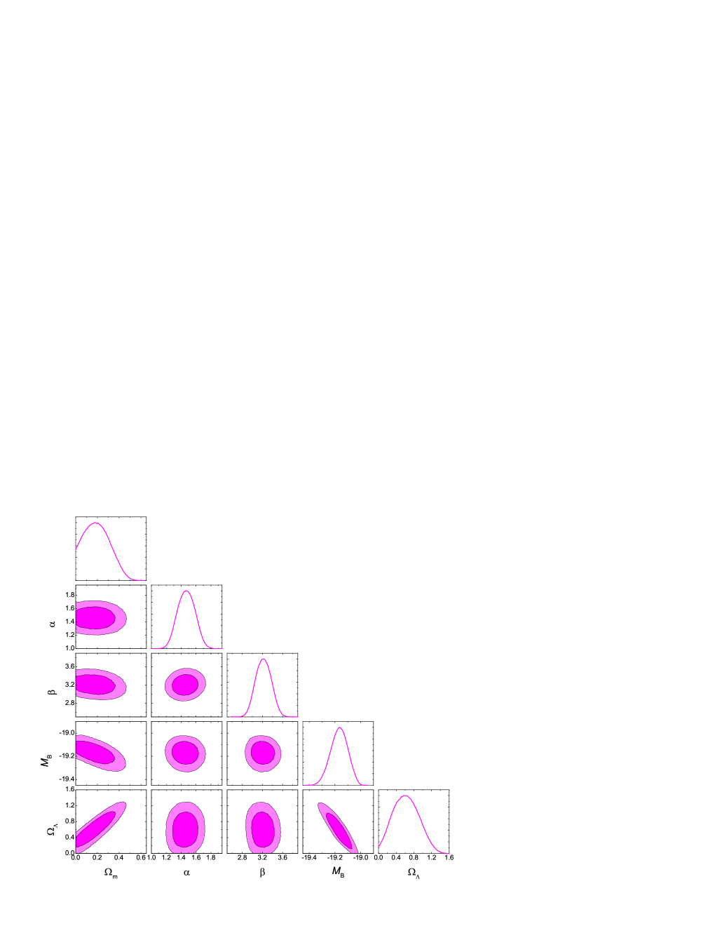
Figure 2: The (normalized) likelihood distributions and 2-D joint distributions with $1\sigma,2\sigma$ contours, for the coefficients $\alpha,\beta,M_{B}$ in Equation 1 and the cosmological parameters $\Omega_{\rm m},\Omega_{\Lambda}$, obtained from a constrained minimization of $\chi^{2}$ (Method I), without the assumption of flatness.

To ensure that our implementation of Method I is reliable and consistent with the results of Guy et al. (2010), we first examine a simple test case: the flat Universe, in which $\Omega_{\Lambda}=\allowbreak 1-\nobreak\Omega_{\rm m}$, with equation-of-state parameter $w_{\Lambda}=-1$. $\Omega_{\rm m}$ is then the only free cosmological parameter. Guy et al. (2010) found that the assumption of flatness resulted in a value for $\Omega_{\rm m}$ that we now know is inconsistent with that reported by Planck2013 (Ade et al. 2014). Nonetheless, it is useful to begin with this test case because it allows us to compare our results directly with theirs. Applying the above $\chi^{2}$-minimization procedure, we find that the fitted parameters in this case are $\alpha=1.470\pm 0.121$, $\beta=3.207\pm 0.157$, $M_{B}=-19.197\pm 0.031$, and $\Omega_{\rm m}=0.235\pm 0.035$, with $\sigma_{\rm int}=0.090$. In Figure 1 we show the (normalized) likelihood distribution for each parameter ($\alpha,\beta,M_{B};\allowbreak\Omega_{\rm m}$), according to the factor $\exp(-\chi^{2}/2)$, and $1\sigma$,$2\sigma$ contours for the joint distribution of each pair of parameters. For each parameter, the likelihood distribution is well approximated by a Gaussian, and the stated confidence interval is a $68\%$ (i.e., $\pm 1\sigma$) interval for this Gaussian. Using the same method and conditions, Guy et al. (2010) obtained $\alpha=1.487\pm 0.097$, $\beta=3.212\pm 0.128$, $M_{B}=-19.210\pm 0.030$, and $\Omega_{\rm m}=0.215\pm 0.033$, with $\sigma_{\rm int}=0.087$. These results are quite consistent, again attesting to the reliability of our calculation.

To allow for a more realistic fit to the SNLS supernova data, we removed the flatness assumption, and allowed both $\Omega_{\rm m}$ and $\Omega_{\Lambda}$ to be free parameters. By minimizing $\chi^{2}$, we now obtain $\alpha=1.469\pm 0.123$, $\beta=3.209\pm 0.159$, $M_{B}=-19.187\pm 0.068$, and $\Omega_{\rm m}=0.217\pm 0.150$, $\Omega_{\Lambda}=0.718\pm 0.329$, with $\sigma_{\rm int}=0.090$. The (normalized) likelihood distribution for each parameter ($\alpha,\beta,M_{B};\allowbreak\Omega_{\rm m},\Omega_{\Lambda}$), and a contour plot for each two-parameter combination, are shown in Figure 2. Dropping the flatness condition, i.e., fitting both $\Omega_{m}$ and $\Omega_{\Lambda}$, makes the best-fit $\Lambda$CDM model marginally consistent with the Planck2013 results, because the $1\sigma$ standard errors are now considerably larger than in the previous case.

It should be noted that the $\chi^{2}$ approach of Method I does not actually maximize a likelihood. Rather, it calculates a value for $\sigma_{\rm int}$ (with no accompanying uncertainty) by requiring that $\chi^{2}_{\rm dof}$ equal unity. Driving $\chi^{2}_{\rm dof}$ to unity, irrespective of how well the cosmological model fits the data, makes it impossible to perform a fair comparison of competing models by using Method I, especially when they have different numbers of parameters. A statistically valid analysis must estimate error dispersion parameter(s), along with all other parameters, by maximizing a joint likelihood function.

Method II. As a superior alternative to Model I for estimating cosmological parameters, and (simultaneously) the model-specific optimized nuisance parameters $\alpha,\beta,M_{B}$, we employ a method described in D’Agostini (2005) and Kim (2011), which is based on the maximization of a joint likelihood function. The joint likelihood function for all these parameters and the intrinsic dispersion $\sigma_{\rm int}$, based on a flat Bayesian prior, is

$$L=\prod_{i}\frac{1}{\sqrt{2\pi(\sigma^{2}_{{\rm lc},i}+\sigma^{2}_{\rm int})}}\;\times\exp\left[-\,\frac{\left(\mu_{B,i}-\mu_{\rm th}(z_{i})\right)^{2}}{2(\sigma^{2}_{{\rm lc},i}+\sigma^{2}_{\rm int})}\right]\propto\exp\left(-\chi^{2}/2\right).$$ (8)

As in Method I, each distance modulus $\mu_{B,i}$ depends on $\alpha,\beta,M_{B}$, and the theoretical distance modulus $\mu_{{\rm th}}(z_{i})$ depends on the cosmological parameters. Maximum likelihood estimation (MLE) is, of course, a standard statistical procedure, and appeared in Method I in a limited way, as a minimization of $\chi^{2}$. The new feature in Method II is that $\sigma_{\rm int}$ is treated on the same level as the other parameters: the likelihood $L$ is maximized over all parameters, now including $\sigma_{\rm int}$. This ‘full MLE’ provides a statistically founded method for estimating $\sigma_{\rm int}$ (Kim 2011). It also treats on the same level the cosmological parameter uncertainties and the potential uncertainty in $\sigma_{\rm int}$, which can affect each other.

The optimized $\Lambda$CDM parameters obtained by Method II are: $\alpha=1.275\pm 0.120$, $\beta=2.637\pm 0.155$, $M_{B}=-19.165\pm 0.081$, $\Omega_{\rm m}=0.365\pm 0.137$, and $\Omega_{\Lambda}=0.846\pm 0.353$, with $\sigma_{\rm int}=0.103\pm 0.010$. For each parameter, the likelihood distribution is well approximated by a Gaussian, and the stated confidence interval is a $68\%$ (i.e., $\pm 1\sigma$) interval for this Gaussian. As anticipated by Kim (2011), these best-fit values are not all consistent with those of Method I, though the estimated value of $\Omega_{\rm m}$ and its error are entirely consistent with the Planck2013 results. In an analysis using mock samples, Kim concluded that differences such as these arise because the commonly used method based on the constrained minimization of $\chi^{2}$ (i.e., Method I) does not include in its error propagation the covariance of $\sigma_{\rm int}$ with the other parameters.

The Method II values of the coefficients $\alpha,\beta,M_{B}$ may now be used to calculate the distance modulus $\mu_{B}$ of Equation 1, for each SN. From the distance moduli, we construct the Hubble diagram shown in the upper panel of Figure 3. We also show the corresponding SNLS sample of 234 Type Ia SNe. As is now well known, the theoretical fit is excellent. The maximum value of the joint likelihood function is given by $-2\ln L=-238.40$, which we shall need when comparing models using the Bayes Information Criterion (see below). For completeness, Figure 3 also shows the Hubble diagram residuals corresponding to the best-fit $\Lambda$CDM model. The likelihood distribution obtained by Method II for each parameter ($\alpha,\beta,M_{B};\allowbreak\Omega_{\rm m},\Omega_{\Lambda};\sigma_{\rm int}$), and a contour plot of the joint distribution for each two-parameter combination, are shown in the lower panel.

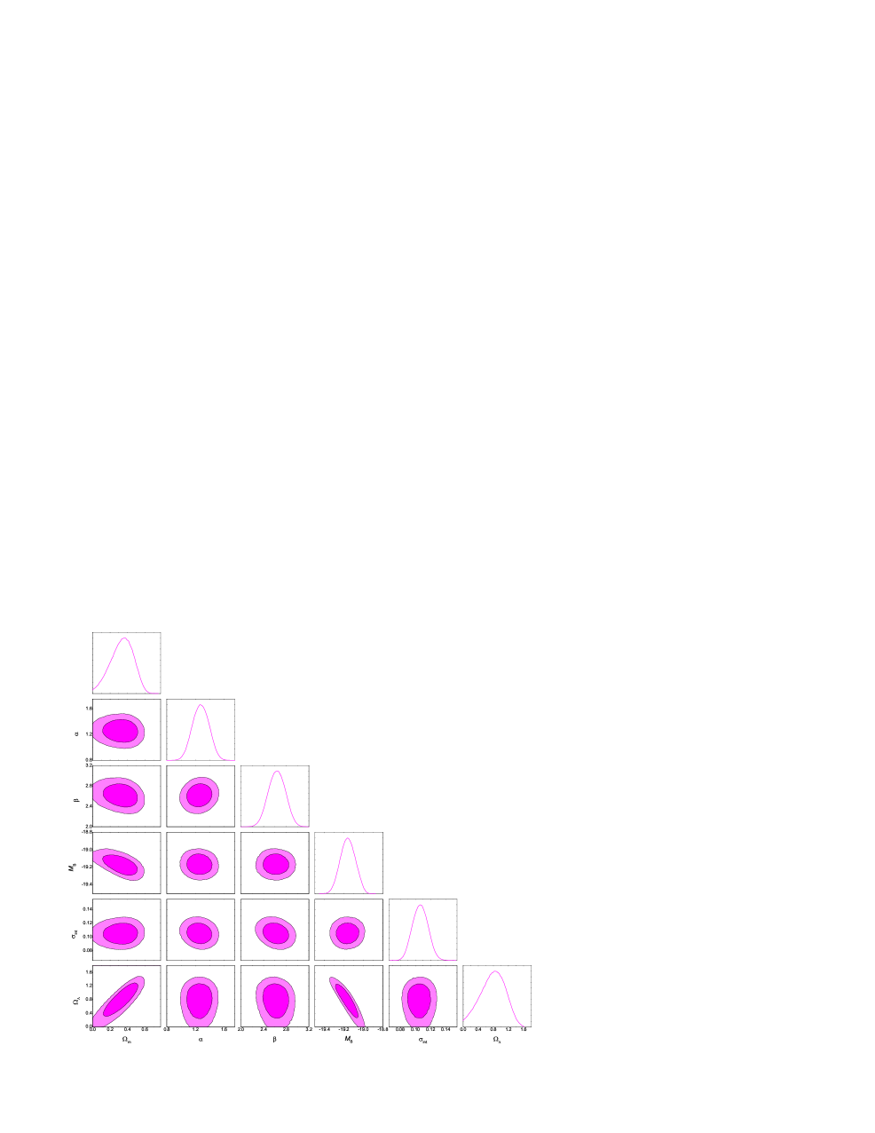
Figure 3: Upper panel: Hubble diagram and Hubble diagram residuals for the SNLS sample of 234 Type Ia SNe in $\Lambda$CDM. Solid curve: best-fit model with $\Omega_{\rm m}=0.365$, $\Omega_{\Lambda}=0.846$ and $p_{\Lambda}=-\rho_{\Lambda}$. Lower panel: (normalized) likelihood distributions and 2-D joint distributions with $1\sigma,2\sigma$ contours, for the coefficients $\alpha,\beta,M_{B}$, the intrinsic dispersion $\sigma_{\rm int}$, and $\Omega_{\rm m},\Omega_{\Lambda}$. The fitting method employed is MLE (Method II).

4 A Direct Comparison Between $\Lambda$CDM and the $R_{\rm h}=ct$ Universe

In the $R_{\rm h}=ct$ Universe, there is only one free parameter: the Hubble constant $H_{0}$. But since we cannot vary $M_{B}$ and $H_{0}$ separately, there are no free parameters left to adjust the theoretical curve, once we optimize $M_{B}$ as one of the nuisance parameters characterizing the supernova luminosities.

Table 1: Best Fits for Different Cosmological Models

Model	$\alpha$	$\beta$	$M_{B}$	$\sigma_{\rm int}$	$\Omega_{\rm m}$	$\Omega_{\Lambda}$	$-2\ln L$	BIC
Method I
$\Lambda$CDM ($k=0$)	$1.470\pm 0.121$	$3.207\pm 0.157$	$-19.197\pm 0.031$	$0.090\qquad\quad\;$	$0.235\pm 0.035$	$1-\Omega_{\rm m}\qquad\;\;$	—	—
$\Lambda$CDM	$1.469\pm 0.123$	$3.209\pm 0.159$	$-19.187\pm 0.068$	$0.090\qquad\quad\;$	$0.217\pm 0.150$	$0.718\pm 0.329$	—	—
Method II
$\Lambda$CDM	$1.275\pm 0.120$	$2.637\pm 0.155$	$-19.165\pm 0.081$	$0.103\pm 0.010$	$0.365\pm 0.137$	$0.846\pm 0.353$	-238.40	-205.67
$R_{\rm h}=ct$	$1.175\pm 0.115$	$2.608\pm 0.149$	$-18.959\pm 0.011$	$0.106\pm 0.010$	—	—	-231.85	-210.03

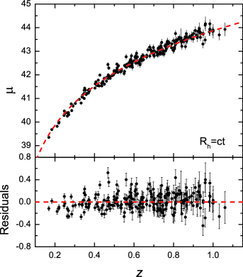
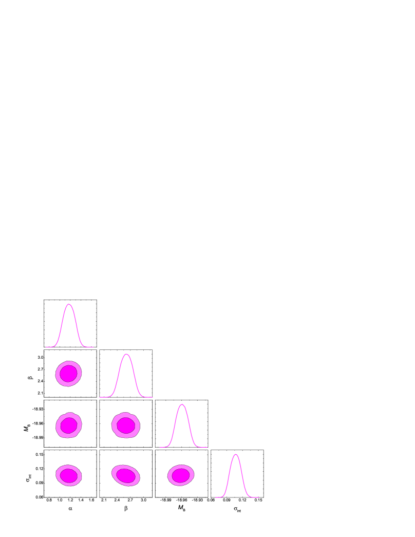
Figure 4: Same as Figure 3, but now for the $R_{\rm h}=ct$ Universe. Upper panel: Hubble diagram and Hubble diagram residuals for the data optimized for $R_{\rm h}=ct$, and the corresponding theoretical curve. Lower panel: The (normalized) likelihood distributions and 2-D joint distributions with $1\sigma,2\sigma$ contours, for all fitted parameters. The fitting method employed is MLE (Method II).

Using the MLE approach (Method II), we find that for the $R_{\rm h}=ct$ Universe, the optimized nuisance parameters are $\alpha=1.175\pm 0.115$, $\beta=2.608\pm 0.149$, $M_{B}=-18.959\pm 0.011$, with $\sigma_{\rm int}=0.106\pm 0.010$. All likelihood distributions are well approximated by Gaussians, and the given confidence intervals are $68\%$ (i.e., $\pm 1\sigma$) intervals for the Gaussians. As with $\Lambda$CDM, we plot the (normalized) likelihood distribution for each parameter ($\alpha,\beta,M_{B};\sigma_{\rm int}$), and 2-D plots for two-parameter combinations (Figure 4). The best-fit values are quite similar to those for $\Lambda$CDM, but are not exactly the same, reaffirming the importance of reducing the data separately for each model being tested. The $R_{\rm h}=ct$ distance modulus is compared to the SNLS sample in the upper panel of Figure 4. For completeness, we also show the Hubble diagram residuals corresponding to the $R_{\rm h}=ct$ Universe at the bottom of this panel. The maximum value of the joint likelihood function for the optimized $R_{\rm h}=ct$ fit corresponds to $-2\ln L=-231.85$. All the fits performed in this paper are summarized in Table 1, for ease of comparison.

An inspection of the Hubble diagrams in Figures 3 and 4 reveals that the distance moduli are slightly different when the nuisance parameters are optimized using different models, but both $\Lambda$CDM and $R_{\rm h}=ct$ fit their respective data sets very well. One certainly gets this impression from a side-by-side comparison of the Hubble-diagram residuals for the SNLS sample in $\Lambda$CDM and $R_{\rm h}=ct$, shown in Figure 5. However, because these models formulate their observables (such as the luminosity distance in Equations 3 and 5) differently, and because they do not have the same number of free parameters, a decision between the models must be based on a formal model selection technique, and in this regard, the results of our analysis favor $R_{\rm h}=ct$ over $\Lambda$CDM, as we shall now demonstrate quantitatively.

A companion paper (Melia & Maier 2013) discussed at length how one may use state-of-the art model selection tools to choose the model to be preferred in accounting for the data. We shall not reproduce that discussion here, but we do point out that to assess competing models in cosmology, a strong case for using the Bayes Information Criterion (BIC) has been made (see, e.g., Liddle 2004, 2007; Liddle et al. 2006). The BIC is applicable when data points are independent and identically distributed, which is a reasonable assumption for supernova redshift–luminosity data. The method has now been used to compare several popular models against $\Lambda$CDM (see, e.g., Shi et al. 2012).

       

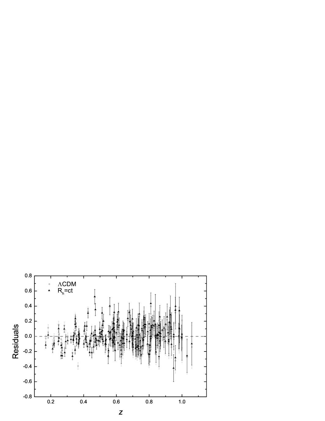
Figure 5: A side-by-side comparison of the Hubble-diagram residuals for the SNLS sample in the standard ($\Lambda$CDM) model and the $R_{\rm h}=ct$ Universe.

Despite its name, the BIC is based not on information theory, but rather on an asymptotic ($n\to\infty$, where $n$ is the number of data points) approximation to the outcome of a Bayesian inference procedure for deciding between competing models (Schwarz 1978). A comparison between the BIC values of two or more fitted models provides their relative ranks, and also a numerical measure of confidence (a likelihood or posterior probability) that each model is the best. Unlike some model selection techniques, the BIC can be applied to ‘non-nested’ models, such as those we have here. The BIC for a fitted regression model, linear or nonlinear, captures the dominant (in the $n\to\infty$ limit) behavior of the associated Bayes factor, which assesses the strength of the evidence in its favor (Kass & Raftery 1995, § 4.1). In this limit, it is only subdominant terms that are affected by such considerations as the choice of a Bayesian prior (Kuha 2004), or the extent of the model nonlinearity if any (Haughton 1988). There is accordingly a simple formula for the BIC, namely

$${\rm BIC}=-2\ln L+(\ln n)k\;,$$ (9)

where $k$ is the number of fitted parameters. The logarithmic penalty term in the BIC strongly suppresses overfitting if $n$ is large (the situation we have here, with $n=234$, which is deep in the asymptotic regime).

A quantitative ranking of fitted models 1 and 2 is computed as follows. If ${\rm BIC}_{\alpha}$ comes from model $\alpha$, the unnormalized confidence in this model is the ‘Bayes weight’ $\exp(-{\rm BIC}_{\alpha}/2)$. That is, in the light of the data, model $\alpha$ has likelihood

$$P(\alpha)=\frac{\exp(-{\rm BIC}_{\alpha}/2)}{\exp(-{\rm BIC}_{1}/2)+\exp(-{\rm BIC}_{2}/2)}$$ (10)

of being the correct choice. The strength of the evidence for model 1 and against model 2 is quantified by $\Delta{\rm BIC}\equiv\allowbreak{\rm BIC}_{2}-\nobreak{\rm BIC}_{1}$, and the following qualitative interpretation of $\Delta{\rm BIC}$ is standard. If $\Delta{\rm BIC}$ is less than $2$, the evidence is “not worth more than a bare mention” (Kass & Raftery 1995). If it is in the range $2\dots 6$, the evidence is positive; if it is in the range $6\dots 10$, the evidence is strong; and if it is greater than $10$, the evidence is very strong.

With $n=234$ data points and $k=4$ parameters, the BIC for the optimized $R_{\rm h}=ct$ Universe is ${\rm BIC}_{1}=-210.03$. For the optimized $\Lambda$CDM, with $k=6$, the corresponding value is ${\rm BIC}_{2}=-205.67$. Our analysis therefore shows that the evidence supplied by the SNLS sample for the $R_{\rm h}=ct$ Universe over $\Lambda$CDM is positive; and quantitatively, $R_{\rm h}=ct$ is favored over $\Lambda$CDM with a likelihood of $\sim 90\%$ versus only $\sim 10\%$.

5 Discussion and Conclusions

Our comparative analysis of $\Lambda$CDM and the $R_{\rm h}=ct$ Universe using the SNLS sample has shown that—contrary to earlier claims—the Type Ia SNe do not point to an expansion history of the Universe in conflict with that implied by other kinds of source, such as the cosmic chronometers (Jimenez & Loeb 2002; Simon et al. 2005; Stern et al. 2010; Moresco et al. 2012; Melia & Maier 2013), GRBs (Norris et al. 2000; Amati et al. 2002; Schaefer 2003; Wei & Gao 2003; Yonetoku et al. 2004; Ghirlanda et al.  2004; Liang & Zhang 2005; Liang et al. 2008; Wang et al. 2011; Wei et al. 2013), and high-$z$ quasars (Kauffmann & Haehnelt 2000; Wyithe & Loeb 2003; Hopkins et al. 2005; Croton et al. 2006; Fan 2006; Willott et al. 2003; Jiang et al. 2007; Kurk et al. 2007; Tanaka & Haiman 2009; Lippai et al. 2009; Hirschmann et al. 2010; Melia 2013a). A difficulty with the use of supernova data has always been their dependence on the underlying cosmology. There is no question that to compare different models properly, one must optimize the nuisance parameters describing the supernova luminosities separately for each expansion scenario. It is not appropriate to use data optimized for $\Lambda$CDM to test other models.

This has been the primary focus of our analysis in this paper. We have confirmed the argument made by Kim (2011), in particular, that one should optimize parameters by carrying out a maximum likelihood estimation in any situation where the parameters include an unknown intrinsic dispersion. The commonly used method, which estimates the dispersion by requiring the reduced $\chi^{2}$ to equal unity, does not take into account all possible covariances among the parameters. In this regard, our best-fit models for $\Lambda$CDM do not agree exactly with those of Guy et al. (2010), who optimized the model parameters using only Method I. Indeed, while their best-fit model is characterized by parameters noticeably different from those of Planck2013, we have demonstrated that the use of Method II actually results in an optimized $\Lambda$CDM model consistent with that based on the analysis of the CMB fluctuations. Simply based on a consideration of the standard model, therefore, our results support the proposal made by Kim (2011) that Method II should be preferred over Method I in the analysis of Type Ia SN samples that include unknown intrinsic dispersions.

More importantly, we have found that, when the parameter optimization is handled via the joint likelihood function, both $\Lambda$CDM and $R_{\rm h}=ct$ fit their individually optimized data very well. However, the $R_{\rm h}=ct$ Universe has only one free parameter—the Hubble constant $H_{0}$—which enhances the significance of the fit over that using $\Lambda$CDM. Indeed, standard model selection techniques penalize models with a large number of free parameters. We have found that the BIC favors $R_{\rm h}=ct$ over $\Lambda$CDM, by a likelihood of $\sim 90\%$ versus $\sim 10\%$. The difference in likelihoods would be even greater for other variations of $\Lambda$CDM that include a larger number of free parameters, e.g., to characterize the dark-energy equation-of-state, should $w_{\Lambda}$ not be constant.

This result would be quite significant on its own. But when we consider it in concert with the analysis of all the other data sets that have been analyzed thus far, it is reasonable to conclude that $R_{\rm h}=ct$ is a more accurate representation of the Universe than is $\Lambda$CDM. This has far-reaching consequences that will be addressed at greater length elsewhere.

Obviously, these results call into question the conclusion that the Universe is currently undergoing a period of acceleration, following an earlier period of deceleration. The fact that the fits to the data using $\Lambda$CDM often come very close to those of $R_{\rm h}=ct$ (see Figure 5) lends weight to our suspicion that the standard model functions as an empirical approximation to the latter, since it has more free parameters and lacks that essential ingredient in $R_{\rm h}=ct$: the equation-of-state $p=-\rho/3$. In attempting to identify the reasons why $\Lambda$CDM produces phases of acceleration and deceleration, one is reminded of trying to fit a straight line with a low-order polynomial—it is always possible to make the ends meet, but there will be inevitable wiggles in between. It appears that the early deceleration and current acceleration indicated by $\Lambda$CDM are two of these wiggles, whereas $R_{\rm h}=ct$ fits the straight line perfectly.

In this work, we have also demonstrated that the class of Type Ia SNe continues to be critical to our understanding of how the Universe evolves, the results reported here affirming the expectation from theory and general relativity that only a perfect fluid with zero active mass (i.e., ${\rho+3p=0}$) can be consistent with the use of an FRW metric (Melia 2013b).

References

- Ade et al. (2014) Ade, P. A. R. et al. 2014, A&A, 571, article id A23, 48 pp.
- Amanullah et al. (2010) Amanullah, R., Lidman, C., Rubin, D., et al. 2010, ApJ, 716, 712
- Amati et al. (2002) Amati, L., Frontera, F., Tavani, M., et al. 2002, A&A, 390, 81
- Bennett, C. L. et al. (2003) Bennett, C. L. et al. 2003, ApJS, 148, 97
- Birkhoff, G. D. (1923) Birkhoff, G. D. 1923, Relativity and Modern Physics, Harvard Univ. Press
- Croton et al. (2006) Croton, D. J. et al. 2006, MNRAS, 365, 11
- D’Agostini (2005) D’Agostini, G. 2005, arXiv:physics/0511182
- Dawson et al. (2009) Dawson, K. S., Aldering, G., Amanullah, R., et al. 2009, AJ, 138, 1271
- De Rosa et al. (2011) De Rosa, G., Decarli, R., Walter, F., et al. 2011, ApJ, 739, 56
- Fan (2006) Fan, X. 2006, New Astronomy Review, 50, 665
- Garnavich et al. (1998) Garnavich, P. M., Jha, S., Challis, P., et al. 1998, ApJ, 509, 74
- Ghirlanda et al. (2004) Ghirlanda, G., Ghisellini, G., & Lazzati, D. 2004, ApJ, 616, 331
- Guy et al. (2010) Guy, J. et al. 2010, A&A, 523, A7
- Haughton (1998) Haughton, D. M. A. 1988, Ann. Statist., 16, 342
- Hirshmann et al. (2010) Hirschmann, M., Khockfar, S., Burkert, A., Naab, T., Genel, S. & Somerville, R. S. 2010, MNRAS, 407, 1016
- Holz & Linder (2005) Holz, D. E., & Linder, E. V. 2005, ApJ, 631, 678
- Hopkins et al. (2005) Hopkins, P. F., Hernquist, L., Cox, T. J., Di Matteo, T., Martini, P. Robertson, B. & Springel, V. 2005, ApJ, 630, 705
- Jiang et al. (2007) Jiang, L. et al. 2007, AJ, 134, 1150
- Jimenez et al. (2002) Jimenez, R. & Loeb, A. 2002, ApJ, 573, 37
- Kass & Raftery (2005) Kass, R. E. & Raftery, A. E. 1995, J. Amer. Statist. Assoc., 90, 773
- Kauffmann & Haehnelt (2000) Kauffmann, G. & Haehnelt, M. 2000, MNRAS, 311, 576
- Kim (2011) Kim, A. G. 2011, PASP, 123, 230
- Kowalski et al. (2008) Kowalski, M., Rubin, D., Aldering, G., et al. 2008, ApJ, 686, 749
- Kuha (2004) Kuha, J. 2004, Sociol. Methods Res., 33, 188
- Kurk et al. (2007) Kurk, J. D. et al. 2007, ApJ, 669, 32
- Kuznetsova et al. (2008) Kuznetsova, N., Barbary, K., Connolly, B., et al. 2008, ApJ, 673, 981
- Liang & Zhang (2005) Liang, E., & Zhang, B. 2005, ApJ, 633, 611
- Liang et al. (2008) Liang, N., Xiao, W. K., Liu, Y., & Zhang, S. N. 2008, ApJ, 685, 354
- Liddle et al. (2006) Liddle, A., Mukherjee, P., & Parkinson, D. 2006, Astronomy and Geophysics, 47, 040000
- Liddle (2007) Liddle, A. R. 2007, MNRAS, 377, L74
- Liddle (2004) Liddle, A. R. 2004, MNRAS, 351, L49
- Lippai et al. (2009) Lippai, Z., Frei, Z. & Haiman, Z. 2009, ApJ, 701, 360
- Melia (2007) Melia, F. 2007, MNRAS, 382, 1917
- Melia (2012) Melia, F. 2012a, AJ, 144, 110
- Melia (2012) Melia, F. 2012b, Australian Physics, 49, 83 (arXiv:1205.2713)
- Melia (2013) Melia, F. 2013a, ApJ, 764, 72
- Melia (2014) Melia, F. 2013b, Annals of Physics, submitted
- Melia & Abdelqader (2009) Melia, F. & Abdelqader, M. 2009, IJMP-D, 18, 1889
- Melia & Maier (2013) Melia, F., & Maier, R. S. 2013, MNRAS, 432, 2669
- Melia & Shevchuk (2012) Melia, F., & Shevchuk, A. S. H. 2012, MNRAS, 419, 2579
- Misner & Sharp (1964) Misner, C. W. & Sharp, D. H. 1964, Phys. Rev., 136, 571
- Moresco et al. (2012) Moresco, M., et al. 2012, JCAP, 8, article id 006, 41 pp.
- Norris et al. (2000) Norris, J. P., Marani, G. F., & Bonnell, J. T. 2000, ApJ, 534, 248
- Perlmutter et al. (1998) Perlmutter, S., Aldering, G., della Valle, M., et al. 1998, Nature, 391, 51
- Perlmutter et al. (1999) Perlmutter, S., Aldering, G., Goldhaber, G., et al. 1999, ApJ, 517, 565
- Riess et al. (1998) Riess, A. G., Filippenko, A. V., Challis, P., et al. 1998, AJ, 116, 1009
- Riess et al. (2011) Riess, A. G., Macri, L., Casertano, S., et al. 2011, ApJ, 730, 119
- Schaefer (2003) Schaefer, B. E. 2003, ApJ, 583, L71
- Schmidt et al. (1998) Schmidt, B. P., Suntzeff, N. B., Phillips, M. M., et al. 1998, ApJ, 507, 46
- (50) Schwarz, G. 1978, Ann. Statist., 6, 461
- (51) Shafieloo, A., Kim, A. G. and Linder, E. V. 2012, PRD, 85, 123530
- Shi et al. (2012) Shi, K., Huang, Y. F., & Lu, T. 2012, MNRAS, 426, 2452
- Simon et al. (2005) Simon, J., Verde, L., & Jimenez, R. 2005, Phys. Rev. D, 71, 123001
- Stern et al. (2010) Stern, D., Jimenez, R., Verde, L., Stanford, S. A., & Kamionkowski, M. 2010, ApJS, 188, 280
- Suzuki et al. (2012) Suzuki, N., Rubin, D., Lidman, C., et al. 2012, ApJ, 746, 85
- Tanaka & Haiman (2009) Tanaka, T. & Haiman, Z. 2009, ApJ, 696, 1798
- Wang et al. (2011) Wang, F.-Y., Qi, S., & Dai, Z.-G. 2011, MNRAS, 415, 3423
- Wei & Gao (2003) Wei, D. M., & Gao, W. H. 2003, MNRAS, 345, 743
- Wei et al. (2013) Wei, J.-J., Wu, X.-F., & Melia, F. 2013, ApJ, 772, 43
- Weyl, H. (1923) Weyl, H. 1923, Z. Phys., 24, 230
- Willott et al. (2003) Willott, C. J., McLure, R. J. & Jarvis, M. J. 2003, ApJ Letters, 587, L15
- Willott et al. (2010) Willott, C. J., Albert, L., Arzoumanian, D., et al. 2010a, AJ, 140, 546
- Willott et al. (2010) Willott, C. J., Delorme, P., Reylé, C., et al. 2010b, AJ, 139, 906
- Wyithe & Loeb (2003) Wyithe, J. S. B. & Loeb, A. 2003, ApJ, 595, 614
- Yonetoku et al. (2004) Yonetoku, D., Murakami, T., Nakamura, T., et al. 2004, ApJ, 609, 935