Dark jets in solar coronal holes

Abstract

A new solar feature termed a dark jet is identified from observations of an extended solar coronal hole that was continuously monitored for over 44 hours by the EUV Imaging Spectrometer on board the Hinode spacecraft in 2011 February 8–10. Line-of-sight velocity maps derived from the coronal Fe xii $\lambda$195.12 emission line, formed at 1.5 MK, revealed a number of large-scale, jet-like structures that showed significant blueshifts. The structures had either weak or no intensity signal in 193 Å filter images from the Atmospheric Imaging Assembly on board the Solar Dynamics Observatory, suggesting that the jets are essentially invisible to imaging instruments. The dark jets are rooted in bright points and occur both within the coronal hole and at the quiet Sun–coronal hole boundary. They exhibit a wide range of shapes, from narrow columns to fan-shaped structures, and sometimes multiple jets are seen close together. A detailed study of one dark jet showed line-of-sight speeds increasing along the jet axis from 52 to 107 km s^-1 and a temperature of 1.2–1.3 MK. The low intensity of the jet was due either to a small filling factor of 2% or to a curtain-like morphology. From the HOP 177 sample, dark jets are as common as regular coronal hole jets, but their low intensity suggests a mass flux around two orders of magnitude lower.

1 Introduction

Coronal jets are a striking feature of solar coronal hole observations obtained at X-ray or extreme ultraviolet (EUV) wavelengths (Shimojo et al., 1996; Cirtain et al., 2007; Nisticò et al., 2009). They are identified through a transient, collimated structure that appears in image sequences and thus, by definition, have an enhanced intensity over their background. In this work we show examples of jets that are essentially invisible in EUV image sequences, but have a clear signature in Dopplergrams derived from an EUV emission line. We refer to these events as dark jets.

Jets are a fundamental type of energy-release process on the Sun, with a relatively simple observational signature. As such they have been the subject of extensive theoretical study ranging from the early 2D simulations of Shibata & Uchida (1986) and Yokoyama & Shibata (1995), to more recent 3D simulations of Miyagoshi & Yokoyama (2003), Pariat et al. (2009) and Moreno-Insertis & Galsgaard (2013). The jets represent an outflow of plasma that is believed to be driven by magnetic field evolution, and flux emergence is the most commonly-modeled scenario (Yokoyama & Shibata, 1995; Moreno-Insertis & Galsgaard, 2013) although observations suggest that flux cancellation often leads to jets (Liu et al., 2011; Young & Muglach, 2014a, b).

The modern observatories Hinode and the Solar Dynamics Observatory (SDO) have led to many new jet studies, particularly for coronal hole jets (CHJs). The X-Ray Telescope (XRT) on board Hinode sees many more CHJs than previous X-ray instruments (Cirtain et al., 2007; Savcheva et al., 2007), principally due to enhanced sensitivity at lower temperatures. Coverage has also been expanded by the Atmospheric Imaging Assembly (AIA) on board SDO which obtains full-disk solar images in a number of EUV filters at a continuous, high time-cadence. Examples of CHJs from AIA were presented by Shen et al. (2011) and Hong et al. (2013), and the present work follows on from the work of Young & Muglach (2014a, b) who combined SDO imaging data with spectroscopic data from the EUV Imaging Spectrometer (EIS) on board Hinode.

The present paper is structured as follows. Sect. 2 describes the observations; Sect. 3 presents three examples of dark jets, demonstrating their lack of an intensity signature; Sect. 4 provides a detailed analysis of one of the dark jets; and results are summarized in Sect. 5.

2 Observations

The dark jets discussed in the present work were identified from a data-set obtained through Hinode Operation Plan (HOP) No. 177, which was run over a 44.4 hour period from 2011 Feburary 8 10:22 UT to February 10 06:47 UT. The jets are identified from Hinode/EIS data and SDO/AIA images are used for comparison. AIA is described by Lemen et al. (2012) and we mostly use images from the 193 Å filter, which we refer to as “A193”. This filter is dominated by emission from Fe xii in most conditions (O’Dwyer et al., 2010) and so is the best comparison with the EIS Fe xii $\lambda$195.12 emission line. The images are obtained at a 12 second cadence and we bin groups of five images together in order to boost signal-to-noise, giving a cadence of 1 minute. For studying the evolution of the bright points at the bases of the dark jets, we consider A193 images for the period $\pm 20$ minutes either side of the time when EIS observed the jets. The EIS instrument (Culhane et al., 2007) performed 43 raster scans with the study Large_CH_Map, which performed a scan over a field-of-view 179″ $\times$ 512″ with the 2${{}^{\prime}}{{}^{\prime}}$ slit at 3${{}^{\prime}}{{}^{\prime}}$ step sizes and with 60 second exposure times.

The EIS data were calibrated using the standard options recommended in the EIS data-analysis guide and the Fe xii $\lambda$195.12 emission line was fit with a Gaussian function at each spatial pixel in the rasters. This line was selected as it is the strongest coronal emission line, in terms of detected photons, in EIS coronal hole spectra due to the high instrument sensitivity at this wavelength. From the line fits, images of intensity, line-of-sight (LOS) velocity and line width were created. The velocity maps revealed 35 spatial features within the coronal hole that exhibited blue-shifts of at least 15 km s^-1 over an extended spatial area. Each feature was present in only a single EIS raster, and so their lifetimes were less than 62 minutes (the cadence of the rasters). Twenty-four of the features could be classified as jets in that they exhibited collimated structures aligned roughly radially from Sun center. AIA 193 Å images were studied in order to identify dynamic phenomena related to the jets. For 13 events we could identify collimated intensity structures that matched the morphology of the EIS velocity structures, and two examples were studied by Young & Muglach (2014a, b). There remained 11 events that showed collimated, jet-like structure in the velocity maps but for which there was not a clear intensity signal in the A193 images. Since jets are typically identified from image sequences through their intensity enhancement then we refer to jets identified through a velocity signature as “dark jets”.

The locations of the 35 blue-shifted features found from the EIS dopplergrams are plotted on an A193 image in Figure 1. The image was obtained by averaging 10 consecutive A193 images between February 8 23:59 UT and February 9 00:01 UT, and the locations of the EIS events have been corrected for the solar rotation. The blue line on Figure 1 shows the coronal hole boundary as determined by the SPOCA code (Delouille et al., 2012), made available through the Heliophysics Event Registry (Hurlburt et al., 2012). We note that the coronal hole has a significant amount of mixed polarity, leading to quite large bright points such as the bright feature at position $(-380,-670)$. We believe that this is a bright point within the coronal hole rather than a quiet Sun region that intrudes into the coronal hole. This is based on the low A193 intensity seen all around the bright point. As will be discussed in the following section, this bright point produced a number of dark jets.

Further details on the full range of jet events identified from HOP 177 are available at the website http://pyoung.org/jets/hop177, which also contains movies for all of the dark jets discussed here. We proceed in the next section to present three examples of dark jets.

3 Dark jet examples

Figure 1 shows the locations of all of the 35 blue-shifted features found from the HOP 177 data-set. Circles show the locations of jets that have an A193 signature, and crosses show features that were not classified as jets due to a lack of a collimated structure. Dark jets are identified with triangles, except for the three jets labeled 1, 2 and 3. These three jets are discussed in more detail below. Of the 11 dark jets, two came from a location on the coronal hole boundary, two came from a small bright point, and seven came from a large feature that we call a bright point complex. Details of the times and positions of these jets are given in Table 3. Each of the 35 blue-shifted features were assigned an index number ordered according to the time the features were observed, and the indices of the 11 dark jets are given in Table 3. Dopplergrams derived from Fe xii $\lambda$195.12 for each of the dark jet locations are shown in Figure 2. These images – derived by fitting a Gaussian to $\lambda$195.12 and converting the centroid to a velocity by comparing with the average centroid over the whole raster – show a wide range of morphology. Events 18, 23 and 30 show long, narrow structures; events 3 and 15 show broad jets; events 25 and 29 actually consist of multiple jets close together; and event 28 has a very complex structure that extends over 100${{}^{\prime}}{{}^{\prime}}$ in length. Below we consider three of the events, and compare the EIS features with A193 image sequences.

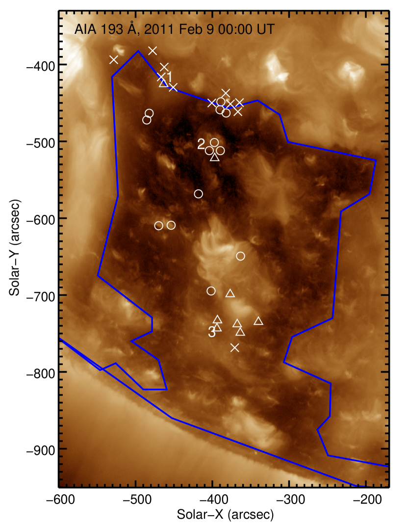
Figure 1: An A193 image from 00:00 UT on February 9, with a logarithmic intensity scaling applied. The symbols and numbers mark the location of 35 blue-shifted features identified from the HOP 177 data-set. Their locations have been differentially-rotated to match the image time. Coronal hole jets are marked with circles; dark jets are marked with triangles or numbers; other blue-shifted features are marked with crosses. The blue line indicates the coronal hole boundary determined by the SPOCA code (Delouille et al., 2012).

Table 1: EIS dark jets from HOP 177.

Index	Date	Time	RN	(X,Y)
3	8-Feb	13:13	3	($-530$,$-420$)
4		15:58	6	($-465$,$-505$)
5		16:16	6	($-515$,$-425$)
15		23:59	14	($-340$,$-735$)
18	9-Feb	01:07	15	($-390$,$-745$)
21		04:12	18	($-370$,$-515$)
23		07:23	21	($-365$,$-730$)
25		08:18	22	($-335$,$-735$)
28		10:25	24	($-330$,$-695$)
29		11:26	25	($-320$,$-745$)
30		13:42	27	($-350$,$-740$)

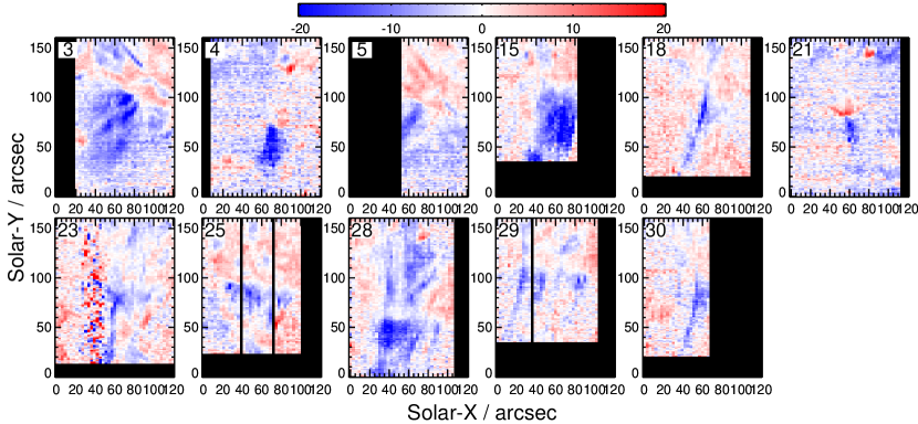
Figure 2: Fe xii $\lambda$195.12 dopplergram images of all of the dark jets identified from the HOP 177 data-set, with indices from Table 3. LOS velocities in the range $-20$ to $+20$ km s^-1 are shown, and each image has a size of $120\times 150$ arcsec².

Figure 3 shows images from a dark jet that EIS rastered over at around 13:13 UT on February 8. It occurred near the coronal hole boundary (which can be seen in the top-right corner of the images). A bright point can be seen in the $\lambda$195.12 intensity image (Figure 3b), and the A193 image (Figure 3a) resolves the bright point into a number of small loops. The EIS velocity image (Figure 3c) shows extensive blue-shifts at the bright point and extending radially away from it. The A193 1-minute cadence movie and the difference image movie (Figure 4) show that the bright point is quite dynamic, but there is no clear evidence of a jet or jets coming from the bright point that could be responsible for the blue-shifts seen in the EIS data. The bright point was present for about two days from 12 UT on February 7, and the A193 emission remained rather weak and diffuse over this period.

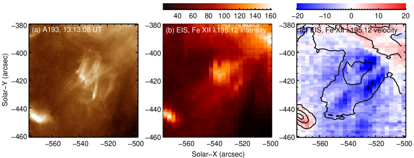
Figure 3: Images of a dark jet observed at 13:13 UT on February 8. Panel (a) shows an A193 image averaged from five consecutive images obtained over 60 seconds. Panels (b) and (c) show intensity (units: erg cm^-2 s^-1 sr^-1) and LOS velocity (units: km s^-1) images derived from performing Gaussian fits to Fe xii $\lambda$195.12.

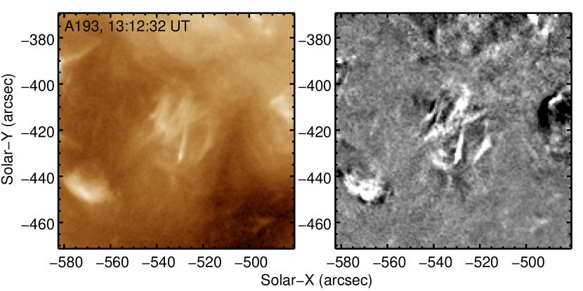
Figure 4: A single image from a movie available in the online edition of the journal, showing the evolution of the bright point that gives rise to the dark jet shown in Figure 3. The left panel shows a A193 image with a logarithmic intensity scaling applied, and the right panel shows a difference movie where the mean image over the 40-image sequence is subtracted from the left-hand image.

The second dark jet example comes from a small bright point that is isolated within the coronal hole. The bright point was present for around two days, and it gave rise to a number of jets including the blowout jet described in Young & Muglach (2014b), which was caused by the cancelation of the main polarities of the bright point leading to its eventual disappearance. The blowout jet occurred at 09:00 UT on February 9, and the dark jet presented here was observed at 15:58 UT on February 8. Figure 5 shows a clear jet-like feature in the velocity map, but with no counterpart in the A193 image or EIS $\lambda$195.12 intensity image. Neither the A193 image movie nor the difference movie (Figure 6) show any structures extending away from the bright point that can be identified with the EIS velocity feature. We note that another dark jet from the same bright point was captured by EIS at 04:12 UT on February 9.

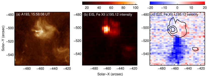
Figure 5: Images of a dark jet observed at 15:58 UT on February 8. Panel (a) shows an A193 image averaged from five consecutive images obtained over 60 seconds. Panels (b) and (c) show intensity (units: erg cm^-2 s^-1 sr^-1) and LOS velocity (units: km s^-1) images derived from performing Gaussian fits to Fe xii $\lambda$195.12.

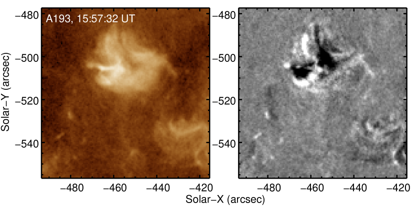
Figure 6: A single image from a movie available in the online edition of the journal, showing the evolution of the bright point that gives rise to the dark jet shown in Figure 5. The left panel shows a A193 image with a logarithmic intensity scaling applied, and the right panel shows a difference movie where the mean image over the 40-image sequence is subtracted from the left-hand image.

Figure 7 shows the third example of a dark jet, which is evident as a blue collimated structure in panel c. The EIS raster is truncated on the right-hand side due to lost telemetry packets during the observation. The jet originates in a region of complex morphology, and in Figure 8 we show a larger A193 field-of-view with the EIS jet location identified. There is an intense bright point at $(-325,-610)$ with larger, more diffuse loops related to this bright point in the region $Y=-700$ to $-620$. There is another patch of emission around $(-355,-720)$ that may be a distinct bright point. It is not clear if the jet is from this bright point or if it has some connection to the large, diffuse loops. The A193 movie and difference-movie (Movie 9) do not show evidence for an intensity structure that matches the EIS velocity jet.

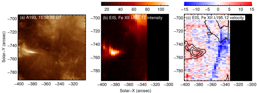
Figure 7: Images of a dark jet observed at 13:42 UT on February 9. Panel (a) shows an A193 image averaged from five consecutive images obtained over 60 seconds. Panels (b) and (c) show intensity (units: erg cm^-2 s^-1 sr^-1) and LOS velocity (units: km s^-1) images derived from performing Gaussian fits to Fe xii $\lambda$195.12.

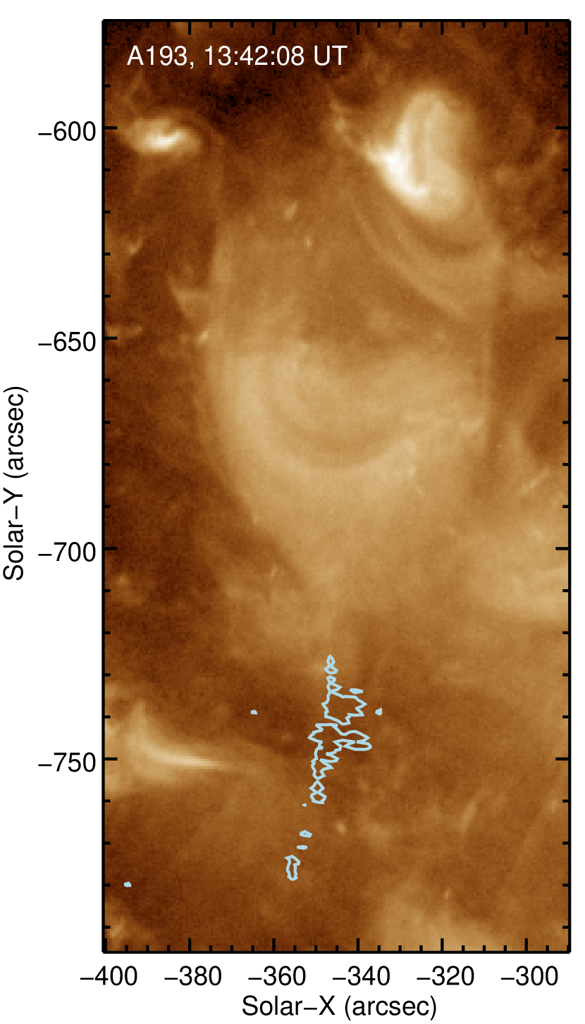
Figure 8: An A193 image from February 9 13:42:08 UT with a logarithmic intensity scaling. The light blue contours show EIS Doppler velocities of $-10$ km s^-1, showing the location of the dark jet from Figure 7.

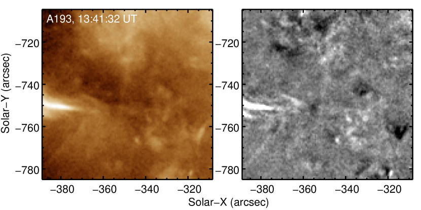
Figure 9: A single image from a movie available in the online edition of the journal, showing the evolution of the bright point that gives rise to the dark jet shown in Figure 7. The left panel shows a A193 image with a logarithmic intensity scaling applied, and the right panel shows a difference movie where the mean image over the 40-image sequence is subtracted from the left-hand image.

4 The February 8 15:58 UT jet

In this section we take a closer look at the dark jet that occurred on February 8 at 15:58 UT (Figures 5, 6). The jet is chosen as it has the simplest geometry, belonging to an isolated bright point in the coronal hole.

Firstly we note that the morphology of the blue feature in the velocity map (Figure 5c) is suggestive of a coronal hole plume, and an A171 image (Figure 10a) does show some diffuse emission extending from the bright point that could be plume plasma. (Polar plumes are known to have temperatures close to the formation temperature of the Fe ix $\lambda$171.1 emission line.) Therefore the $\lambda$195.12 outflow could represent outflowing plume plasma. This can be discounted, however, because the $\lambda$195.12 velocity feature is only seen in a single raster, implying a lifetime of $<62$ minutes, whereas plumes are known to have lifetimes of the order of a day (see review of Wilhelm et al., 2011). In addition, since plumes have temperatures of 0.7–1.1 MK (Wilhelm et al., 2011) then the implied outflowing plasma would be best seen in emission lines formed at this temperature. EIS observes Fe ix $\lambda$197.86 and Figures 10b,c show intensity and velocity images formed from this line. Since it is much weaker than $\lambda$195.12 it was necessary to rebin the data into $2\times 3$ pixels, but Figure 10c clearly shows that there is no velocity feature to compare with that of $\lambda$195.12. Note that the statistical uncertainties on the $\lambda$197.86 velocities are $\approx\pm 5$ km s^-1.

Figure 6 demonstrated that an intensity signature of the dark jet could not be seen in an A193 image sequence. The remaining AIA EUV filter image sequences (94, 131, 171, 211, 304 and 335 Å) were also checked, but no signature was found. Although Hinode X-Ray Telescope data were available for this event, the filters (thin-beryllium and titanium-poly) were not suitable for studying the faint jet emission, and only the bright point could be seen. Previous XRT jet studies (Cirtain et al., 2007; Savcheva et al., 2007) used the aluminium-poly filter which has a better response to low temperature plasmas.

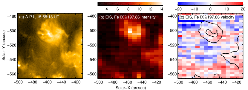
Figure 10: Panel (a) shows an A171 image averaged from five consecutive images obtained over 60 seconds for the dark jet on February 9, 15:58 UT (Figure 5). Panels (b) and (c) show intensity (units: erg cm^-2 s^-1 sr^-1) and LOS velocity (units: km s^-1) images derived from performing Gaussian fits to Fe ix $\lambda$197.86

Inspection of $\lambda$195.12 profiles shows that the dark jet blueshift seen in Figure 5c is due to an asymmetry in the profile caused by extra emission on the short-wavelength side of the line. As the jet occurs within the coronal hole background, then the line profile is a composite of the background and jet emission. To isolate the jet component we subtract out the background component with a technique illustrated in Figures 11 and 12. Four spatial regions were identified: one in the coronal hole background neighboring the jet (Figure 11a), and three along the axis of the jet (Figure 11b). Averaged spectra from each region were obtained using the IDL routine EIS_MASK_SPECTRUM. The keyword /SHIFT was applied, which shifts the spectrum at each spatial pixel onto a common wavelength scale. In particular this accounts for offsets that arise due to the thermal drift and slit tilt found in the EIS data (Kamio et al., 2010). Figure 12a shows the spectrum from jet region 2, with the background region spectrum overplotted. The background-subtracted spectrum for jet region 2 is shown in Figure 12b, clearly revealing a Gaussian-shaped feature that represents the jet plasma. The intensity, width and velocity of this feature for the jet regions 1–3 are given in Table 2. Note that the velocity of this component was derived by assuming that $\lambda$195.12 in the background spectrum is at rest.

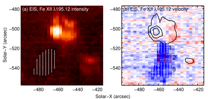
Figure 11: The left panel shows an EIS intensity image from Fe xii $\lambda$195.12 for the February 8 15:58 UT jet. The region selected as the coronal hole background is indicated. The right panel shows the Fe xii $\lambda$195.12 Dopplergram for the same jet, and three regions along the jet’s axis are indicated.

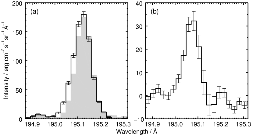
Figure 12: The left panel shows the averaged EIS spectrum from jet region 2 (Figure 11b), with the spectrum from the coronal hole background region (Figure 11a) over-plotted in gray. The right panel shows the spectrum derived by subtracting the background spectrum from the jet spectrum. Error bars are derived from Poisson statistics.

The jet velocities are derived relative to the position of $\lambda$195.12 in the background spectrum. The velocity of the jet component increases along the length of the jet from $-52$ to $-104$ km s^-1, a behavior consistent with the findings of Young & Muglach (2014a, b) for two blowout jets and which suggests that material continues to be accelerated along the jet. The intensities assume the original laboratory radiometric calibration of EIS (Lang et al., 2006). The revised calibration of Del Zanna (2013) does not modify the $\lambda$195.12 intensities, whereas the revised calibration of Warren et al. (2014) reduces the intensities by a factor of 0.85. The line widths have been corrected for the EIS instrumental width (Young, 2011), and are larger than the thermal width at $\log\,T=6.2$ (the temperature of maximum emission of $\lambda$195.12), which is 23 mÅ, although there is no clear pattern when comparing with the background width.

Density measurements of the jet plasma are not possible as the density-sensitive line $\lambda$186.88 (actually a blend of two Fe xii lines at 186.85 and 186.89 Å) could not be measured in the subtracted jet spectra. The values listed in Table 2 are obtained from the un-subtracted jet spectra. The calibration of Warren et al. (2014) was used to determine the densities, and we note that the Del Zanna (2013) calibration would lead to marginally higher values, while the original laboratory calibration leads to values about 0.2–0.3 dex lower. Comparing to the background density value, there is no indication that the jet has an enhanced density over the background. Atomic data for computing the densities were obtained from version 7.1 of the CHIANTI atomic database (Dere et al., 1997; Landi et al., 2013).

The only lines that retained a measurable intensity after background subtraction had been performed were $\lambda$195.12 and the Fe xi lines at 188.22 and 188.30 Å that are blended. We can use the ratio of Fe xii to Fe xi to derive a temperature, and the values are given in Table 2. Atomic data were taken from the CHIANTI atomic database. It can be seen that the jet plasma is a little cooler than the background plasma, but the difference is small. It is clear that the jet plasma is not appreciably hotter or cooler than the background coronal hole plasma.

Table 2: Parameters for a dark jet and coronal hole background.

Region	Intensity	Velocity	Width	$\log\,(N_{\rm e}/{\rm cm}^{-3})$	$\log\,(T/{\rm K})$
	(erg cm-2 s-1 sr-1)	(km s-1)	(mÅ)
Background	$14.7\pm 0.1$	0	$45\pm 3$	$9.33\pm 0.07$	$6.13\pm 0.01$
Region 1	$6.5\pm 0.4$	$-52\pm 4$	$94\pm 6$	$8.85\pm 0.10$	$6.11\pm 0.01$
Region 2	$2.8\pm 0.2$	$-83\pm 5$	$39\pm 7$	$9.06\pm 0.12$	$6.08\pm 0.02$
Region 3	$2.2\pm 0.2$	$-107\pm 5$	$54\pm 5$	$9.18\pm 0.08$	$6.11\pm 0.03$

The mass flux in the jet can be compared with the typical proton mass flux at 1 AU of 2–$4\times 10^{8}$ cm^-2 s^-1 (Feldman et al., 1978). Assuming a filling factor of 1 within the jet, the particle flux is given by $0.85N_{\rm e}v$, where $N_{\rm e}$ is the electron number density, 0.85 is the fraction of protons relative to electrons, and $v$ the velocity along the jet axis. The heliocentric location of the jet bright point is $(-455,-500)$, so if we assume the jet is perpendicular to the solar surface, then the jet is inclined $45^{\circ}$ to the line-of-sight. If we take a mean LOS velocity of 80 km s^-1 (Table 2), then this implies $v\approx 110$ km s^-1. The density of the jet plasma can not be measured separately from the background plasma, but assuming $\log\,N_{\rm e}=9$ gives a proton flux of $9.4\times 10^{15}$ cm^-2 s^-1. The EIS data do not allow accurate estimates of jet lifetimes or frequencies, but the number of dark jets (11) is comparable to the number of regular jets (13) in the HOP 177 data-set. If we assume the regular jets are the same as the X-ray jets discussed by Cirtain et al. (2007), then we expect 10 jets per hour, with average lifetimes of 10 minutes (Savcheva et al., 2007). Assuming these numbers apply to the dark jets, then we expect 1.7 jets on the Sun at any instant. The cross-sectional area of the dark jet can be estimated at 80 Mm² from the size of the structure in the EIS image (Figure 5c). This then gives a proton flux at 1 AU estimate of $2\times 10^{11}$ cm^-2 s^-1. However, the very low intensity of the dark jet is not consistent with the projected size and density. From an average intensity of 3.8 erg cm^-2 s^-1 sr^-1, a density of $\log\,N_{\rm e}=9$ and temperature $\log\,T=6.1$ (Table 2) we can use the CHIANTI database to estimate a column depth of the emitting plasma of only 100 km, compared to the projected jet diameter of 5 Mm. This implies either a low filling factor of only 2% or that the jet is actually a thin “curtain” of emission. The proton flux is then modified to $4\times 10^{9}$ cm^-2 s^-1. This value compares to $4\times 10^{11}$ cm^-2 s^-1 for X-ray jets (Cirtain et al., 2007), and $1.2\times 10^{15}$ cm^-2 s^-1 from spicules (Athay & Holzer, 1982).

The dark jet mass flux estimate contains many assumptions, but it suggests the mass flux is two orders of magnitude smaller than that for regular coronal hole jets. To improve the dark jet estimate would require (i) measurements of dark jet lifetimes using high cadence spectral scans, and (ii) a determination of the relative frequency of regular jets and dark jets.

5 Summary

A continuous 2-day observation by the Hinode/EIS instrument of a large coronal hole extension during 2011 February 8–10 has revealed a number of jet events that are identified only through a Doppler signature in the Fe xii $\lambda$195.12 line (formed at 1.5 MK), with no counterpart in image sequences obtained by the AIA instrument on board SDO. These jets are named dark jets. Of 24 jets identified from the EIS data, 11 are classed as dark jets suggesting a significant fraction of jet events are missed in surveys performed with imaging instruments. The low intensity of the dark jets, however, means that the total mass flux may be up to two orders of magnitude lower than that from regular jets.

The dark jet dopplergram images show a wide range of morphologies, but the dark jets are always associated with bright points, a feature in common with regular jets. The lifetime of the dark jets cannot be constrained from EIS data due to the low cadence of the rasters, but they do not live longer than the 62 minute cadence of the EIS rasters.

An analysis of one dark jet observed by EIS on February 8 at 15:58 UT revealed the following properties:

• The intensity enhancement of the dark jet plasma compared to the background plasma in the Fe xii $\lambda$195.12 line decreases from 44% to 15% along the length of the jet.

• No evidence is found for a density enhancement compared to the background plasma, for which the density is $2.14\times 10^{9}$ cm^-3.

• The temperature of the dark jet plasma is 1.2–1.3 MK.

• The LOS velocity of the dark jet plasma increases with height from $-52$ to $-107$ km s^-1, suggesting that acceleration continues along the jet axis.

• The low jet intensity implies either a low filling factor (2%) for the jet, or a curtain-like structure.

The properties of this dark jet are similar to those of the two regular coronal jets presented by Young & Muglach (2014a, b). In particular, these jets had temperatures of 1.3 and 1.7 MK, respectively, and densities of 1.3 and 2.8 $\times$ $10^{8}$ cm^-3. In addition all three jets showed an increasing speed with height, although the speeds were about a factor two lower for the dark jet. The implied curtain-like structure of the dark jet also matches that of the Young & Muglach (2014b) jet, which had a much smaller line-of-sight width compared to the plane-of-sky width. One difference is that regular coronal jets generally correspond to a major change to the source bright point, such as a strong brightening or morphology change. The bright points underneath dark jets generally do not exhibit obvious changes before or during the jet. These facts suggest that dark jets may be triggered by a smaller-scale, less-energetic mechanism than regular coronal jets, although the mechanism itself (such as magnetic reconnection) may be the same, thus giving rise to similar plasma parameters.

References

- Athay & Holzer (1982) Athay, R. G., & Holzer, T. E. 1982, ApJ, 255, 743
- Cirtain et al. (2007) Cirtain, J. W., et al. 2007, Science, 318, 1580
- Culhane et al. (2007) Culhane, J. L., et al. 2007, Sol. Phys., 243, 19
- Del Zanna (2013) Del Zanna, G. 2013, A&A, 555, A47
- Delouille et al. (2012) Delouille, V., Mampaey, B., Verbeeck, C., & de Visscher, R. 2012, ArXiv e-prints
- Dere et al. (1997) Dere, K. P., Landi, E., Mason, H. E., Monsignori Fossi, B. C., & Young, P. R. 1997, A&AS, 125, 149
- Feldman et al. (1978) Feldman, W. C., Asbridge, J. R., Bame, S. J., & Gosling, J. T. 1978, J. Geophys. Res., 83, 2177
- Hong et al. (2013) Hong, J.-C., Jiang, Y.-C., Yang, J.-Y., Zheng, R.-S., Bi, Y., Li, H.-D., Yang, B., & Yang, D. 2013, Research in Astronomy and Astrophysics, 13, 253
- Hurlburt et al. (2012) Hurlburt, N., et al. 2012, Sol. Phys., 275, 67
- Kamio et al. (2010) Kamio, S., Hara, H., Watanabe, T., Fredvik, T., & Hansteen, V. H. 2010, Sol. Phys., 266, 209
- Landi et al. (2013) Landi, E., Young, P. R., Dere, K. P., Del Zanna, G., & Mason, H. E. 2013, ApJ, 763, 86
- Lang et al. (2006) Lang, J., et al. 2006, Appl. Opt., 45, 8689
- Lemen et al. (2012) Lemen, J. R., et al. 2012, Sol. Phys., 275, 17
- Liu et al. (2011) Liu, C., Deng, N., Liu, R., Ugarte-Urra, I., Wang, S., & Wang, H. 2011, ApJ, 735, L18
- Miyagoshi & Yokoyama (2003) Miyagoshi, T., & Yokoyama, T. 2003, ApJ, 593, L133
- Moreno-Insertis & Galsgaard (2013) Moreno-Insertis, F., & Galsgaard, K. 2013, ApJ, 771, 20
- Nisticò et al. (2009) Nisticò, G., Bothmer, V., Patsourakos, S., & Zimbardo, G. 2009, Sol. Phys., 259, 87
- O’Dwyer et al. (2010) O’Dwyer, B., Del Zanna, G., Mason, H. E., Weber, M. A., & Tripathi, D. 2010, A&A, 521, A21
- Pariat et al. (2009) Pariat, E., Antiochos, S. K., & DeVore, C. R. 2009, ApJ, 691, 61
- Savcheva et al. (2007) Savcheva, A., et al. 2007, PASJ, 59, 771
- Shen et al. (2011) Shen, Y., Liu, Y., Su, J., & Ibrahim, A. 2011, ApJ, 735, L43
- Shibata & Uchida (1986) Shibata, K., & Uchida, Y. 1986, Sol. Phys., 103, 299
- Shimojo et al. (1996) Shimojo, M., Hashimoto, S., Shibata, K., Hirayama, T., Hudson, H. S., & Acton, L. W. 1996, PASJ, 48, 123
- Warren et al. (2014) Warren, H. P., Ugarte-Urra, I., & Landi, E. 2014, ApJS, 213, 11
- Wilhelm et al. (2011) Wilhelm, K., et al. 2011, A&A Rev., 19, 35
- Yokoyama & Shibata (1995) Yokoyama, T., & Shibata, K. 1995, Nature, 375, 42
- Young (2011) Young, P. R. 2011, EIS Software Note No. 7, ver. 1
- Young & Muglach (2014a) Young, P. R., & Muglach, K. 2014a, PASJ
- Young & Muglach (2014b) Young, P. R., & Muglach, K. 2014b, Sol. Phys., 289, 3313