Minimal paths between communities induced by geographical networks

Abstract

In this work we investigate the betweenness centrality in geographical networks and its relationship with network communities. We show that vertices with large betweenness define what we call characteristic betweenness paths in both modeled and real-world geographical networks. We define a geographical network model that possess a simple topology while still being able to present such betweenness paths. Using this model, we show that such paths represent pathways between entry and exit points of highly connected regions, or communities, of geographical networks. By defining a new network, containing information about community adjacencies in the original network, we describe a means to characterize the mesoscale connectivity provided by such characteristic betweenness paths.

I Introduction

As a consequence of their potential to represent real systems, complex networks have become the subject of growing interest in recent years Strogatz (2001). Some examples of systems that have been studied using complex networks are electric power grids Motter et al. (2013), airline routes Lordana et al. (2014), the World-Wide Web Albert and Barabási (2002), among others Newman (2003). Networks whose vertices are embedded in a space with well-defined coordinates and their connectivity is related to the distance between the vertices are named geographical networks Barthélemy (2011). Examples of geographical networks include street, airline, and neural networks. Models to generate artificial networks with geographic dependency have been created Boccaletti et al. (2006) in order to better understand the real systems.

The spatial influence on the connectivity gives rise to many interesting characteristics Costa et al. (2007). In a previous work about the influence of gene expression on neuronal characteristics de Arruda et al. (2015), we computed the betweenness centrality Freeman (1977) of neuronal networks. While visualizing those neuronal networks we observed that the vertices having the highest betweenness centrality values were connected together creating chains of vertices, which here we call betweenness paths. The presence of betweenness paths in the neuronal network suggests a two-level hierarchy of the system structure, where the betweenness paths form the main pathways for information flow and the remaining paths distribute this information locally. Such hierarchical organization has also been observed for road networks Bigotte et al. (2010); Crucitti et al. (2006a, b); Scellato et al. (2006); Yerra and Levinson (2005). In Eppell et al. (2001) its argued that road networks should be planned in different scales, according to their purpose, function or management policies. Such scales range from the entire city level down to local streets used for property access or pedestrian movement. According to Lämmer et al. (2006); Chowell et al. (2003) the traffic in road networks, modeled by applying the betweenness centrality, and the movement of people in a city have also been shown to be power-law distributed, meaning that a few paths concentrate most of the city traffic.

Given that a hierarchical structure of pathways has been observed in a range of systems, it is interesting to study the reasons why they are formed, their importance for the correct operation of the system, their influence in the network flow, and in which kind of geographical networks the betweenness paths can be found. To better understand the hierarchical structures, it is necessary to study how the network topology is inducing those paths. Furthermore, the knowledge about betweenness paths and their characteristics can be used for better planning the system.

In this work, we study street networks composed by two hierarchical levels: a main structure forming the backbone of the network, and secondary connections supported by such backbone. We considered networks generated from geographic models and real-world street networks. From these networks, we identified connected vertices with high betweenness centrality. We observed that these vertices provide a good covering of the topology, in the sense that any network vertex is aways near at least one or more characteristic betweenness paths. We found that such paths tend to be related with the community structure Newman (2006) of the network. So, to better understand the characteristic betweenness paths and its relationship with communities, we created a random geographic model and used community detection to divide the space in well-defined regions. In order to study the relationship between such communities and their geographical positions, we created a sub-summed community network, where each vertex is a different community and the connection weights are based on the amount of shortest paths crossing the community border.

This paper is organized as follows. Section II presents the basic network theory concepts that are used in this paper. In Section III we discuss betweenness paths in network models and real cases. In Section IV we create a network model to better understand the betweenness paths. In Section V, we describe the relationship between geographic and topological measurements.

II Basic concepts

There are many ways to compute network centralities, each being developed to evaluate different network characteristics Boccaletti et al. (2006).

In order to locally quantify the network centrality, it is possible to measure the degree $k_{i}$ for each vertex $i$. Furthermore, in weighted networks, we can consider the edges to define a measurement called strength Costa et al. (2007), which is computed for each vertex $i$ as

$$S_{i}=\sum_{j\in r_{i}}{w_{ij}},$$ (1)

where $r_{i}$ is the set of neighbors of vertex $i$ and $w_{ij}$ is the weight of the edge connecting $i$ to $j$.

The network centrality can also be computed globally, that is, considering the whole network structure. One important global centrality measure is the stress centrality ($SC_{u}$) Shimbel (1953). This measure is defined for each vertex $u$ as

$$SC_{u}=\sum_{ij}{\sigma(i,u,j)},$$ (2)

where $\sigma(i,u,j)$ represents the number of shortest paths between the vertices $i$ and $j$ crossing the vertex $u$. If one vertex is removed from the network it can affect the stress of all other vertices.

Another important global measurement is the betweenness centrality, which also considers the amount of shortest paths crossing a vertices Freeman (1977). This measure is defined as

$$B_{u}=\sum_{ij}\frac{\sigma(i,u,j)}{\sigma(i,j)},$$ (3)

where $\sigma(i,u,j)$ represents the number of shortest paths between the vertices $i$ and $j$ crossing the vertex $u$ and $\sigma(i,j)$ is the total amount of shortest paths between $i$ and $j$. The betweenness centrality can be implemented using a fast algorithm Brandes (2001, 2008), where the betweenness centrality is computed and the result is used to compute the stress centrality.

Betweenness centrality is frequently used to study flows in networks Newman (2005); Borgatti (2005); Freeman et al. (1991) and can be used in several applications. In social networks it can be described in terms of its message communications, considering that each message take the shortest path Newman (2010). In power grid networks, this measure can quantify the load of each vertex Motter and Lai (2002). It is also used in the cascading-failure dynamics Mirzasoleiman et al. (2011).

In addition to the centrality measures, another important concept studied in complex networks theory is the community structure of the system. Where a community is defined as a set of vertices densely interconnected, and with few connections to vertices outside this set. This property can be found in many real networks such as social networks Arenas et al. (2004), metabolic networks Guimera and Amaral (2005), and in the structure of cities Zhong et al. (2014). In city networks, those communities are shown to be subdivisions of urban structure emerging urban elements and their interactions Zhong et al. (2014).

A common approach to quantify how well-defined are the communities in the network is the modularity measure Newman (2006). The modularity is represented as

$$Q=\frac{1}{2m}\sum_{i,j}\left(A_{ij}-\frac{k_{i}k_{j}}{2m}\right)\delta(c_{i},c_{j}),$$ (4)

where $m$ is the number of network edges, $A$ is the network adjacency matrix, $k_{i}$ and $k_{j}$ are the vertex degree $i$ and $j$, respectively, $c_{i}$ and $c_{j}$ are the communities of vertex $i$ and $j$, respectively, and $\delta(c_{i},c_{j})$ is $0$ if $c_{i}\neq c_{j}$ or $1$ if $c_{i}=c_{j}$.

Network communities can be detected through the optimization of modularity. For a comprehensive review of modularity optimization methods, please refere to Fortunato (2010). In this work we use the fast greedy Clauset et al. (2004) algorithm to detect the communities.

III Characteristic betweenness paths

In this section we define and analyze the characteristic betweenness paths. We compute the betweenness centrality of all the vertices. Most of these vertices are connected, creating chains of vertices. Thus, most of them have degree two. We define a betweenness path as a sub-network considering only the the highest betweenness centrality values. In other words we selected only vertices with betweenness centrality higher or equal than a threshold and created a sub-network composed by such vertices. In order to do so, we compute the betweenness centrality of the vertices in a network and divide them into two groups. Vertices having betweenness larger than a threshold $T$ are called characteristic vertices, while the rest of vertices in the network are called secondary vertices.

We will show four networks in which the characteristic paths can be observed. Two of these networks are artificially generated, and the other two are street networks. In the first model, known as Waxman Waxman (1988), the vertices are organized randomly in a plane. For each vertex, the probability to connect with all other vertices follows an exponential decay of the distance between them. In the second model, known as random geometric graph Penrose (2003), the vertices are randomly organized and the connections are created only when the geographical distance is lower than a fixed value. We compared the network models with two real street networks: from San Joaquin County in USA and Oldenburg city in Germany Brinkhoff (2002).

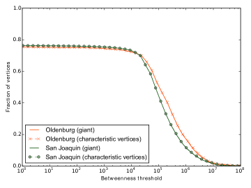
In order to find a reasonable value for the threshold, we computed the fraction of characteristic vertices according to some selected values of betweenness threshold. The fraction is found by dividing the number of characteristic vertices by the size of the network. We perform these tests using the street networks, the results can be seen in Figure 1. Moreover, we also plot in Figure 1 the largest connected component (giant component) of characteristic vertices. The majority of the characteristic vertices are included in the giant component for all different threshold values. Furthermore, the curves are similar for both cities. There is no indication of a proper threshold for defining the characteristic vertices. Therefore, we empirically selected a threshold for which $20\%$ of the network vertices become characteristic vertices. If we consider the subnetwork formed by such vertices and their respective connections it is possible to show that for each analyzed network an interesting structure is obtained. Such structure contains a chain-like connectivity between the characteristic vertices, meaning that the majority of vertices have degree two. Such chain-like structure contains most of the flow in the network, represented by the betweenness, and can be seen as the backbone of the original network. The secondary vertices rely upon this backbone for proper communication with the rest of the system. The characteristic betweenness paths were also found in other works, but their origins were not analyzed Crucitti et al. (2006a, b); Lämmer et al. (2006).

Figure 1: (Color online) The plot shows the fraction of characteristic vertices against the betweenness threshold. For each network we also show the number of characteristic vertices in the giant component.

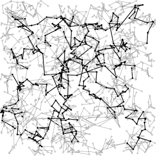
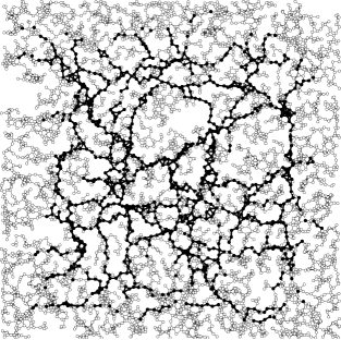
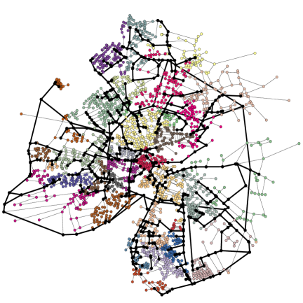
In order to illustrate the betweenness paths, we simulated the Waxman network with 1707 vertices and average degree 2.20 (The network is shown in Figure 2(a)). The random geometric graph has 4883 vertices and average degree 6.18 (as can be shown in Figure 2(b)). The street network from San Joaquin has 14503 vertices and average degree 2.75, and the network representing Oldenburg streets has 2873 vertices and average degree 2.57. The Oldenburg network is shown Figure 2(c), where each color represents a different community. The San Joaquin network is not shown in Figure 2 because the network is very large, which hinders a proper visualization of its paths and communities.

For each network we computed the betweenness centrality and highlighted the 20% of vertices with largest betweenness values, which defines the characteristic betweenness paths. The characteristic betweenness paths occurred in all examples, which are the characteristic vertices. By visual inspection, in each network the characteristic vertices seem to define a backbone structure having many two-degree vertices. Such backbone is formed by what we call the characteristic betweenness paths. In street networks this result can indicate a tendency that the volume of cars is bigger in some streets than in others if we consider that all drivers are using the shortest paths for the formation of high flow streets.

In every example we could observe the characteristic betweenness paths and it was possible to identify more than one component with high betweenness centrality in the same network. The component sizes were different for each network. In the random geometric model, the giant component represents 85% of all vertices in the characteristic path. In the other networks the giant component represents more than 98% of all vertices in the paths.

Figure 2: (Color online) Geographical networks, where black circles and highlighted edges show the preferential paths. Item (a) represents the network of Waxman model, item (b) represents the network of the random geometric model, and item (c) represents the network of Oldenburg streets, where each color represents a different community.

We analyze the coverage of the characteristic paths. In order to do so, we measured the shortest distance between each secondary vertex $i$ and preferential paths (represented as $d_{i}$), because the shorter the distances are, the better are the paths coverage. In order to provide a fair comparison between different networks, the calculated distances are normalized by the average path length, $l$, of each network. Therefore, we define the normalized shortest path distance, $\Theta_{i}$, as

$$\Theta_{i}=\frac{d_{i}}{l}.$$

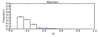
We generate $60$ samples of each model. In this case, we fit the model variables in order to compare with the Oldenburg network (modularity 0.92). The samples of Waxman model have $2976.70\pm 16.61$ vertices, average degree $2.71\pm 0.04$, and modularity $0.79\pm 0.01$. The samples of random geographic model have $2892.33\pm 58.46$ vertices, average degree $4.50\pm 0.09$, and modularity $0.97\pm 0.001$. In order to do a comparison considering the statistical variations of the models, these results are shown as histograms in Figure 3. We observed that the fraction of vertices with the fewer distance (first bin in the histogram) is longer in the random geometric model than the Waxman model comparing the two models, we observe that secondary vertices tend to be closer to characteristic paths in the random geometric graph model, but in this network the longest distance is small than that case (as can be seen in Figures 3(a) and (b)). Furthermore, the standard deviation is smaller in two networks for both models, showing that this effect is not a statistical artifact caused by fluctuation. The shortest distances were also analyzed for the street networks (as can be seen in Figures 3(c) and (d)). The dashed lines represent the average values of $\Theta$, which we call the coverage of the characteristic paths. The coverage of Oldenburg is larger than for San Joaquin, which may be a consequence of the higher complexity of Oldenburg’s topology Brinkhoff (2002).

Figure 3: The histograms show the normalized shortest path distance, $\Theta$, between each secondary vertex and preferential paths. We consider the (a) random geometric model, (b) Waxman model, (c) the Oldenburg network and (d) the San Joaquin network. The dashed lines represent the coverage and error bars in items (a) and (b) shows the standard deviation.

IV Characteristic paths model

In order to better understand the emergence of characteristic paths in geographic networks, we define a model able to generate networks with a simple lattice-like topology, but still containing a well-defined backbone structure. The initial structure of the network is a 2D regular lattice, where the vertices are organized in lines and equally spaced columns. First we defined the size, $L$, of the network (number of lines and columns) and two variables, the maximum distance to connect two vertices as $d_{MAX}$ and a probability $x$ to remove randomly the edges for each vertex. The algorithm follows three steps: 1- The vertices are organized as a square grid with toroidal boundary condition; 2- For each pair of vertices $i$ and $j$ when the distance $d_{ij}$ is less or equal than $d_{MAX}$ an edge connecting $i$ to $j$ is created; 3- Each edge is removed with probability $x$.

In order to visualize the betweenness paths in the model presented in this section, we created a network using the parameter $L=200$, so that the network has $N=40000$. The connectivity range was set to $d_{MAX}=\sqrt{2}$. Therefore, each vertex of the network has degree 8. We randomly remove the connections with probability $x=0.65$.

Figure 4: (Color online) Item (a) presents a heat map showing the betweenness centrality of vertices belonging to a simple realization of our model. The color blue shows regions without vertices. In item (b) each color represents a different community, some distinct, non-adjacent, communities are associated to the same color due to color palette limitations.. The color black shows the preferential paths. The color white shows regions without vertices.

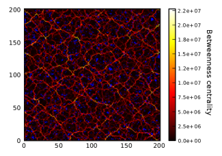
We measured the betweenness centrality for each network vertex and the results can be seen in Figure 4(a). We can observe vertices with higher values (characteristic vertices) generating preferential paths in the network, in a similar manner as main streets. Our hypothesis is that the network communities are inducing the formation of betweenness paths through connections between them. In Figure 4(b) we show the network communities and characteristic paths (indicated in black). The result suggests that the paths are going through communities.

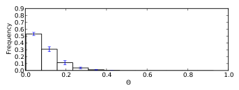
To compare the characteristic betweenness paths displayed by our network model and real networks, we executed the same tests as in the previous section. In order to infer the statistical variation of the model, we created $60$ network samples. We used the parameter $L=56$ and we randomly removed the connections with probability $x=0.7$. These parameters were set so that the generated networks have a size and average degree as close as possible to compare with the Oldenburg network. The network measurements are: number of vertices $2829.95\pm 21.34$, average degree $2.59\pm 0.03$, and modularity $0.94\pm 0.002$.

Our model has similarities and differences from the street networks and the other models. The giant componet represents $(85\pm 8)\%$ of all characteristic vertices. Regarding the shortest distance between secondary vertices and preferential paths (Figure 5), the secondary vertices tend to be more distant from the backbone than in the Oldenburg and Waxman networks.

Figure 5: Histogram of normalized shortest path distance, $\Theta$, between each secondary vertex and preferential betweenness paths.

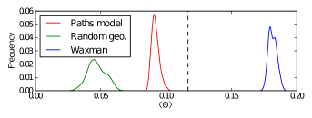
We compared the average of shortest distance between the secondary vertices and the preferential betweenness paths in network models and the Oldenburg network. For each generated network we calculate coverage, which we represent by $\langle\Theta\rangle$, and in Figure 6 we show the distribution of $\langle\Theta\rangle$ for the generated networks. The dashed line shows the coverage for Oldenburg. The coverage for Oldenburg is closest to the measured values for the characteristic path model. Besides, the standard deviation is low, which confirms that the betweenness paths have a similar structure in all generated networks. Therefore, in the following we further analyze the betweenness paths using a single realization of our model.

Figure 6: Histogram of the coverage for $60$ generated networks from each considered model. The dashed line represents the coverage in Oldenburg’s network.

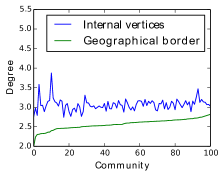
To quantify our network communities in terms of their respective degree and betweenness centrality, we considered two types of vertices, the geographical border community vertices and the internal community vertices. The first type represents vertices that have at least one neighbor in the grid belonging to a different community, no matter if they are connected or not. The second type represents a vertex that is not a geographical border. In order to define each vertex type, we considered all eight geographical neighbors, of the vertices. In some analyses we also considered the topological border community vertices, which are the vertices connected with one or more vertices from different community. We generated a network with $L=200$ and average degree $2.92$ according to our model. Using this network we computed three different comparisons. In the first, we compare the average degree between internal vertices and border community vertices (as can be seen in Figure 7(a)). In this comparison it is possible to observe that the average degree in the internal community vertices is higher than the border community vertices. Thereby, we can affirm that the vertex degree is influencing how the community is formed.

Figure 7: (Color online) Image (a) shows the degree comparison between internal vertices and border community vertices, image (b) shows the degree comparison between topological and geographical border, and image (c) shows the betweenness centrality comparison between topological and geographical border. The community indexes were ordered according to the degree of internal community vertices.

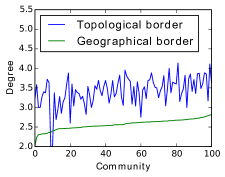
In order to describe how the vertices are connecting communities, we measured the average degree in the geographical community border and in the topological community border, represented in Figure 7(b). In 98% of the communities, the average degree of vertices belonging to the geographical border is lower than for vertices contained in the topological border.

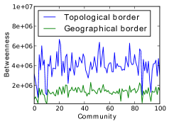
We made a similar comparison, between geographic and topological borders, but now measuring the betweenness centrality instead of the degree (as can be seen in Figure 7(c)). This analysis can show if connections between communities (topological border) are generating a characteristic betweenness paths. Figure 7 shows that the average geographical border betweenness is lower than the topological border betweenness for all communities. Thus, in average, the vertices where the paths are crossing the community borders have higher betweenness centrality and degree than the geographical borders. Some vertices of characteristic paths are part of the topological border. In other words, they are connecting the communities.

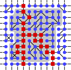
The results indicate that the paths represent routes of efficient communication between the communities. This idea is illustrated in Figure 8. Vertices included in the highlighted gray region belong to the same community. The community has three vertices on its topological border and the shortest paths connecting them, shown in red, are creating the preferential paths with higher betweenness centrality.

Figure 8: (Color online) The highlighted region represents a community and the red squares represent characteristic vertices crossing the community.

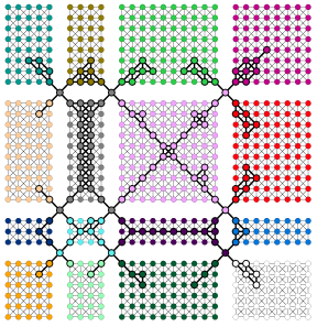
In order to validate these results, we created an artificial geographic network with fixed communities. In this network, each community is a regular lattice, where the vertices are connected with their eight nearest neighbors, and the communities are interconnected through some selected vertices. Figure 9 shows the network and highlight the highest values of betweenness centrality (the characteristic vertices). In this test, it is possible to observe that the characteristic paths are connecting the communities. Besides, through this model, it is possible to note that the paths are not created at random, that is, their emergence have a well-defined mechanism.

Figure 9: (Color online) Network created by connecting lattice-like communities. Each community is represented by a different color and the characteristic paths are highlighted.

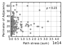
It is also interesting to analyze if the number of shortest paths connecting pairs of communities are related to the sizes of the communities geographical border. In order to do so, we plot the perimeter of adjacency between communities against the sum of the vertex stress connecting such communities, which can be seen in Figure 10. Besides, we calculated the Pearson correlation coefficient between the measurements, obtaining a value of 0.23. Thus, these measurements are uncorrelated.

Figure 10: Scatter plot showing for each community the summation of all stress connecting vertices from a community to another against the perimeter of adjacency. The Pearson correlation ($\rho$) is shown inside the plot.

V Community adjacency network

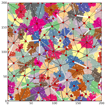
In order to observe the relationship between communities and their importance, considering geographical characteristics, we created a network based on the topological adjacency between communities of our characteristic paths model. Through this model it is possible to compare the geographical characteristics (e.g., the community area) with topological characteristics, such as the degree of a vertex, which represents the number of communities connected with a given community. In this network, each vertex represents a community. A weight equal to $SC_{i}+SC_{j}$ (defined in Equation 2) is associated to each edge connecting communities $i$ and $j$. The resulting network is undirected. In Figure 11 we show a typical realization of this network. It is possible to observe small communities having strong connections, indicating that betweenness paths are also present in such small communities. On the other hand, there are big communities with weak connections, showing that few preferential paths are crossing them.

Figure 11: (Color online) Heat map representing the community adjacency network from communities, where the color of edges represent the weight (black is zero and white is one).

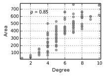
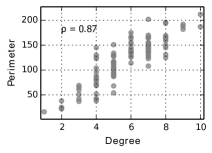
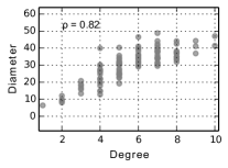
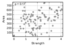
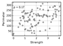
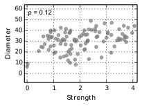
We compared local topology characteristics of the community adjacency network with geometrical characteristics (the scatter plots can be seen in Figure 12). Figures 12(a), (b) and (c) show the degree as a function of area, perimeter and diameter, respectively and Figures 12(d), (e) and (f) show the same measures using the vertex strength instead of the degree. The degree is highly correlated with the geographical characteristics of communities. On the other hand, the strength has little relationship with the communities geometry. This happens because the strength is uncorrelated with the geographical characteristics of communities.

Figure 12: Scatter plots comparing geographical and topological measurements in the community networks. The items (a), (b), and (c) represent the unweighted degree against geographical characteristics and the items (d), (e), and (f) represent the strength against geographical characteristics. The Pearson correlation, $\rho$, is shown inside each plot.

VI Conclusion

The structure of a geographical network has a direct impact on how the system can be navigated. Our analysis revealed that betweenness paths are a common characteristic of geographical networks, since they can be found in geographical models as well as real world networks. We characterized the betweenness paths in terms of the distance between each network secondary vertex and the closest betweenness path. Such measurement can be related to the covering provided by the paths to reach the entire network. We showed that in both the geographical models and the street networks the betweenness paths provide a good covering of the system. In order to better understand the establishment of the characteristic paths, we proposed a model to generate geographical networks having a simple topology but that can still originate such paths.

It was found that the characteristic betweenness paths have a strong relationship with the presence of well-defined communities in the networks. We compared the vertices degrees and betweenness centrality among geographical and topological borders of the communities, as well as the internal vertices of the communities. This analysis revealed that the betweenness characteristic paths are usually induced by the communities, in the sense that such paths provide a communication between entry and exit points of the communities.

The number of shortest paths passing through the topological border of adjacent communities seems to be independent of the geometry of the interface between the communities. This was revealed by the absence of correlation between the total stress of vertices connecting adjacent communities and the perimeter of the adjacency. In order to better understand the relationship between communities and characteristic betweenness paths, we defined a new structure based on the vertices betweenness and the community organization of the network being studied, which we called community network. By characterizing this meta structure, we concluded that geographical characteristics can influence the connectivity between communities, which takes place along betweenness characteristic paths.

It remains an open question if other, non-geographical, network models can also present such characteristic betweenness paths. Also, the proper impact that such paths may have on a dynamics taking place on the system is also an interesting aspect for future studies.

VII acknowledgments

Henrique Ferraz de Arruda thanks CNPq (Grant no. 132363/2013-5) and CAPES for financial support. Cesar Henrique Comin acknowledges FAPESP (Grant no. 11/22639-8) for financial support. Luciano da Fontoura Costa is grateful to CNPq (Grant no. 307333/2013-2), FAPESP (Grants no. 11/50761-2), and NAP-PRP-USP for sponsorship. The authors thanks Filipi Nascimento Silva for fruitful discussions.

References

- Strogatz (2001) S. H. Strogatz, Nature 410, 268 (2001).
- Motter et al. (2013) A. E. Motter, S. A. Myers, M. Anghel, and T. Nishikawa, Nat Phys 9, 191 (2013).
- Lordana et al. (2014) O. Lordana, J. M. Sallana, P. Simoa, and D. Gonzalez-Prietob, Transportation Research Part E: Logistics and Transportation Review 68, 155 (2014).
- Albert and Barabási (2002) R. Albert and A.-L. Barabási, Rev. Mod. Phys. 74, 47 (2002).
- Newman (2003) M. E. J. Newman, SIAM Review 45, 167 (2003).
- Barthélemy (2011) M. Barthélemy, Physics Reports 499, 1 (2011).
- Boccaletti et al. (2006) S. Boccaletti, V. Latora, Y. Moreno, M. Chavez, and D.-U. Hwang, Phys. Rep. 424, 175 (2006).
- Costa et al. (2007) L. da F. Costa, F. A. Rodrigues, G. Travieso, and V. P. R. Boas, Advances in Physics 56, 167 (2007), cond-mat/0505185 .
- de Arruda et al. (2015) H. F. de Arruda, C. H. Comin, M. Miazaki, M. P. Viana, and L. da F. Costa, Journal of neuroscience methods 245, 1 (2015).
- Freeman (1977) L. Freeman, Sociometry 40, 35 (1977).
- Bigotte et al. (2010) J. F. Bigotte, D. Krass, A. P. Antunes, and O. Berman, Transportation Research Part A: Policy and Practice 44, 506 (2010).
- Crucitti et al. (2006a) P. Crucitti, V. Latora, and S. Porta, Phys. Rev. E 73, 036125 (2006a).
- Crucitti et al. (2006b) P. Crucitti, V. Latora, and S. Porta, Chaos: An Interdisciplinary Journal of Nonlinear Science 16, 015113 (2006b).
- Scellato et al. (2006) S. Scellato, A. Cardillo, V. Latora, and S. Porta, The European Physical Journal B-Condensed Matter and Complex Systems 50, 221 (2006).
- Yerra and Levinson (2005) B. M. Yerra and D. M. Levinson, The Annals of Regional Science 39, 541 (2005).
- Eppell et al. (2001) V. Eppell, B. A. McClurg, and J. M. Bunker, (2001).
- Lämmer et al. (2006) S. Lämmer, B. Gehlsen, and D. Helbing, Physica A: Statistical Mechanics and its Applications 363, 89 (2006).
- Chowell et al. (2003) G. Chowell, J. M. Hyman, S. Eubank, and C. Castillo-Chavez, Physical Review E 68, 066102 (2003).
- Newman (2006) M. E. J. Newman, Proceedings of the National Academy of Sciences 103, 8577 (2006).
- Shimbel (1953) A. Shimbel, Bulletin of Mathematical Biophysics 15, 501 (1953).
- Brandes (2001) U. Brandes, Journal of Mathematical Sociology 25 (2001).
- Brandes (2008) U. Brandes, Social Networks 30, 136 (2008).
- Newman (2005) M. E. J. Newman, Social networks 27, 39 (2005).
- Borgatti (2005) S. P. Borgatti, Social networks 27, 55 (2005).
- Freeman et al. (1991) L. C. Freeman, S. P. Borgatti, and D. R. White, Social networks 13, 141 (1991).
- Newman (2010) M. E. J. Newman, Networks: An Introduction (Oxford University Press, Inc., New York, NY, USA, 2010).
- Motter and Lai (2002) A. E. Motter and Y.-C. Lai, Physical Review E 66, 065102 (2002).
- Mirzasoleiman et al. (2011) B. Mirzasoleiman, M. Babaei, M. Jalili, and M. A. Safari, Physical Review E 84, 046114 (2011).
- Arenas et al. (2004) A. Arenas, L. Danon, A. Diaz-Guilera, P. M. Gleiser, and R. Guimera, The European Physical Journal B-Condensed Matter and Complex Systems 38, 373 (2004).
- Guimera and Amaral (2005) R. Guimera and L. A. N. Amaral, Nature 433, 895 (2005).
- Zhong et al. (2014) C. Zhong, S. M. Arisona, X. Huang, M. Batty, and G. Schmitt, International Journal of Geographical Information Science 28, 2178 (2014).
- Fortunato (2010) S. Fortunato, Physics Reports 486, 75 (2010).
- Clauset et al. (2004) A. Clauset, M. E. J. Newman, and C. Moore, Phys. Rev. E 70, 066111 (2004).
- Waxman (1988) B. M. Waxman, IEEE Journal on Selected Areas in Communications 6, 1617 (1988).
- Penrose (2003) M. Penrose, Random Geometric Graphs, Oxford studies in probability (Oxford University Press, 2003).
- Brinkhoff (2002) T. Brinkhoff, Geoinformatica 6, 153 (2002).