Immersed boundary-finite element model of fluid-structure interaction in the aortic root

Abstract

It has long been recognized that aortic root elasticity helps to ensure efficient aortic valve closure, but our understanding of the functional importance of the elasticity and geometry of the aortic root continues to evolve as increasingly detailed in vivo imaging data become available. Herein, we describe fluid-structure interaction models of the aortic root, including the aortic valve leaflets, the sinuses of Valsalva, the aortic annulus, and the sinotubular junction, that employ a version of Peskin’s immersed boundary (IB) method with a finite element (FE) description of the structural elasticity. We develop both an idealized model of the root with three-fold symmetry of the aortic sinuses and valve leaflets, and a more realistic model that accounts for the differences in the sizes of the left, right, and noncoronary sinuses and corresponding valve cusps. As in earlier work, we use fiber-based models of the valve leaflets, but this study extends earlier IB models of the aortic root by employing incompressible hyperelastic models of the mechanics of the sinuses and ascending aorta using a constitutive law fit to experimental data from human aortic root tissue. In vivo pressure loading is accounted for by a backwards displacement method that determines the unloaded configurations of the root models. Our models yield realistic cardiac output at physiological pressures, with low transvalvular pressure differences during forward flow, minimal regurgitation during valve closure, and realistic pressure loads when the valve is closed during diastole. Further, results from high-resolution computations demonstrate that IB models of the aortic valve are able to produce essentially grid-converged dynamics at practical grid spacings for the high-Reynolds number flows of the aortic root.

1 Introduction

The aortic root consists of the three semilunar aortic valve cusps, the three sinuses of Valsalva, which are bulbous cavities positioned behind each valve leaflet, the aortic annulus, where the aortic valve leaflets attach to the aorta, and the sinotubular junction, where the sinuses merge into the ascending aorta. The healthy aortic valve acts to ensure unidirectional flow of oxygenated blood from the heart to the tissues of the body, including to the heart itself via the coronary circulation. Diseases of the aortic valve can result in stenosis or regurgitation, and severe aortic valve disease is treated by repairing or by replacing the diseased valve with either a mechanical or a bioprosthetic valve carr2005 . Approximately 50,000 such procedures are performed each year in the United States freeman2005 ; bonow2006 ; singh2008 . Continuing advances in noninvasive in vivo imaging of blood flow and tissue deformation, mechanical tests specifically targeted to biological tissues, and computer modeling and simulation enable integrative studies of the dynamics and mechanics of the aortic root humphrey2002 . Such work has the potential to improve both medical devices and surgical procedures used to treat patients with valvular heart disease, and also clinical approaches to patient risk assessment and treatment planning.

Aortic compliance, and specifically the compliance of the aortic sinuses, has a fundamental role in the function of the aortic root. The sinuses act as reservoirs, storing blood during systole and then releasing it in diastole to facilitate flow in the coronaries thubrikar1989 . The compliance of the sinuses also helps to ensure the proper closure of the aortic valve bellhouse1968 . Further, the shape of the aortic root causes blood to circulate in the sinuses, generating vortices that act both on the valve leaflets and on the sinus walls. These vortices generate forces that facilitate effective valve closure and act as a regulatory mechanism that synchronizes closure bellhouse1968 . Although this mechanism of efficient valve closure was first postulated by Leonardo da Vinci, there remains some debate in the surgical community about whether it is important to recreate the anatomic geometry of the native aortic root in aortic valve and root replacement procedures cheng2007 .

More recently, our understanding of the functional importance of the elasticity and anatomical geometry of the aortic root has evolved as increasingly detailed data have been acquired on the in vivo deformations that occur during the cardiac cycle. For instance, it has been shown that the aortic root undergoes a multi-modal series of conformational changes even before the leaflets open dagum1999 . It has been argued that these deformations act to reduce shear stresses on the valve leaflets and thereby prolong the life of the native valve leaflets cheng2007 . Annular and commissural flexibility may be a key component in this interaction, and annular flexibility is lost with the implantation of a stented artificial valve, possibly reducing the lifetime of bioprosthetic valve leaflets. The annular commissures also participate in load sharing, which reduces peak stresses on the aortic cusps immediately after valve closure. Devices such as the Medtronic 3f Aortic Bioprosthesis attempt to account for both the annular and the commissural flexibility of the native root, but despite the theoretical advantages offered by such designs, more traditional devices with rigid annuluses still dominate clinical practice.

A challenge in modeling and simulating the mechanical response of arteries, including the aorta, is that the arterial walls are continuously subjected to substantial intraluminal pressures in their in vivo state. Thus, arterial geometries that are derived from in vivo imaging generally correspond to a loaded configuration. In addition, as first demonstrated by Fung fung1983 and by Vaishnav and Vossoughi vaishnav1983 , even the unloaded configuration of the artery is not stress free. Instead, because of tissue growth and remodeling, the arterial wall includes residual stresses and is subject to axial tethering fung1991 ; humphrey2002 ; cardamone2009 . These factors all conspire to make determining the unloaded arterial geometry challenging. Indeed, both the deformation due to intraluminal pressure loading and the residual stresses cannot be measured directly in vivo, and therefore these quantities must be estimated. Residual stresses may be determined from ex vivo experiments, whereas the zero-pressure configuration of blood vessels can be determined by solving the inverse elastostatic problem.

Different approaches have been developed to solve the inverse elastostatic problem for complex arterial geometries derived from medical imaging data. Most of these strategies can be grouped in two broad categories. One group of approaches focuses on retrieving the initial deformation field and the initial stress field of the artery while keeping the imaging-derived geometry unaltered. An example of this type of approach is the modified updated Lagrangian formulation (MULF) introduced by Gee et al. gee2009 , which is an incremental prestressing method that recovers the equilibrium configuration rather than the zero-pressure geometry. A second group of approaches determines an unloaded configuration of the vessel that, when subjected to intraluminal pressure loading, will inflate to match the imaging-derived geometry. Among the first to develop a stationary method to solve the inverse elastostatic problem were Govindjee and Mihalic govindjee1998 . This method was extended by Lu et al. lu2007 to arteries, but this approach does not appear to have been widely used in practice, possibly because it requires a modification in the finite element (FE) solution scheme that renders this method somewhat difficult to implement within commercial FE analysis software. In comparison, the backward incremental method developed by de Putter et al. dePutter2007 requires updating the deformation gradient and thereby can be implemented with fewer modifications to the finite element code. Perhaps the most straightforward approach to retrieving the zero-pressure configuration is the backward displacement method proposed by Bols et al. bols2012 , which iteratively modifies the coordinates of the reference configuration rather than the deformation gradient tensor. We use the backward displacement method in this work to recover the unloaded configuration of an idealized model of the aortic root.

While the methods to obtain an estimation of the zero-pressure configuration of a blood vessel can be applied to any geometry, determining residual stresses is a local, vessel-specific task that presently requires harvesting and then destroying the blood vessel. Computational approaches to accounting for residual stresses are usually based on an assumed ‘open’ configuration, which is subsequently ‘closed,’ thereby reversing the process that releases residual stresses alastrue2007 ; creane2012 . This approach is difficult to apply to noncylindrical geometries and, in particular, cannot be readily applied to imaging-derived geometries creane2012 . A more generic approach to including residual stress in arteries is described in Alastrué et al. alastrue2007 and is based on a Kröner-Lee decomposition of the deformation gradient tensor. For simplicity, we do not consider residual stresses in the present work, although we do account for initial strains resulting from in vivo pressure loading.

Most the methods surveyed above have been developed and applied to study aneurysmal arteries lu2007 ; gee2009 , although applications to normal vessels as well as other pathophysiological conditions are possible. Because arterial wall stress distributions are considered good predictors of aneurysm rupture, improvements in the accuracy of computed wall stress distributions are expected to facilitate improvements in aneurysm rupture prediction. In contrast, although the important role of aortic root compliance in valve closure is well documented croft2010 ; crosetto2011 , many dynamic analyses of the aortic valve tend to focus on the mechanical behavior of the valve leaflets and often model the sinuses and the ascending aorta as rigid griffith2009 ; viscardi2010 ; griffith2012 ; yao2012 or as linear elastic materials conti2010 ; marom2012 , but experimental data azadani2012 show that the sinuses and the ascending aorta exhibit a nonlinear hyperelastic behavior. Examples of nonlinear hyperelastic constitutive models used in fluid-structure interaction simulations of the aortic root can be found in studies by De Hart et al. dehart2003 and by Weinberg and Mofrad weinberg2008 , which both adopt an arbitrary Lagrangian-Eulerian (ALE) approach. The application of ALE fluid-structure interaction schemes to modeling aortic valve dynamics is somewhat limited by the remeshing required by such methods as the structure deforms sotiropoulos2009 . Attempts to tackle this limitation have included restricting the problem to a two-dimensional analysis dumont2004 and the implementation of complex remeshing algorithms in three-dimensional analyses cheng2004 .

An alternative approach to modeling interactions between the blood and the aortic valve and root is offered by Peskin’s immersed boundary (IB) method peskin2002 , which was introduced to simulate cardiac valve dynamics peskin1972 and was subsequently extended to model fluid-structure interaction in the heart and its valves peskin1996 ; mcqueen1997 ; mcqueen2000 ; kovacs2001 ; mcqueen2001 ; griffith2007 ; griffith2009-ib_chapter ; griffith2009 ; griffith2012 ; luo2012 ; ma2013 . This IB approach to fluid-structure interaction is to describe structural stresses and deformations in Lagrangian form, and to describe the momentum, viscosity, and incompressibility of the coupled fluid-structure system in Eulerian form. Integral transforms with Dirac delta function kernels mediate interaction between Lagrangian and Eulerian variables. When discretized, the IB formulation of the equations of motion replaces these singular kernel functions with regularized kernels that are designed to ensure conservation of physical quantities such as force and torque when converting between Lagrangian and Eulerian forms. This numerical approach allows the Lagrangian structural mesh to overlay the background Eulerian grid in an arbitrary manner, thereby avoiding the need to deploy dynamic body-fitted grids. In addition, because the immersed structures move according to a common interpolated velocity field, the IB method offers an implicit contact model that prevents the valve leaflets from interpenetrating, even when subjected to substantial diastolic pressure loads griffith2009 ; griffith2012 . Related sharp-interface IB methods have also been developed and used by Borazjani, Ge, and Sotiropoulos to simulate valvular dynamics for models of both rigid and flexible aortic valve prostheses borazjani2008 ; borazjani2013 . Previous work demonstrated that three-dimensional IB models of the aortic valve can yield physiological cardiac output at realistic pressures griffith2009 ; griffith2012 . However, we are aware of no previous study that demonstrates that the IB method yields reasonably well-resolved simulation results for flexible aortic valve models in three spatial dimensions at practical grid spacings.

The primary aim of this study is to develop new fluid-structure interaction models of the aortic root that substantially extend earlier IB models of aortic valve dynamics griffith2009 ; griffith2012 by including descriptions of the elasticity of the aortic sinuses and the ascending aorta. Herein, the aortic sinuses and proximal ascending aorta are modeled as an incompressible, isotropic, hyperelastic material with an exponential neo-Hookean strain-energy functional humphrey2002 ; delfino1997 that we fit to experimental data obtained by Azadani et al. azadani2012 from human aortic root tissue samples. A separate finite element analysis is employed to estimate the unloaded aortic geometry using a method based on the backward displacement method of Bols et al. bols2012 . Our fluid-structure interaction simulations employ hybrid models of the aortic root that use a fiber-based description of the thin aortic valve leaflets, as done in previous studies griffith2009 ; griffith2012 , along with a finite element-based description griffith-submitted of the comparatively thick walls of the aortic sinuses and proximal ascending aorta.

Two related aortic root models are considered in this work. Each captures the complex interactions between the flow, the thin flexible aortic valve cusps, and the deformable walls of the aortic sinuses and the ascending aorta. The first model employs a highly idealized anatomical geometry, in which the initial and reference configurations of the aortic sinuses and valve cusps are assumed to exhibit three-fold symmetry. The second model employs a more realistic description of the aortic root anatomy that accounts for the differences in the sizes of the left, right, and noncoronary sinuses. Both models are fully three dimensional in the sense that there are no symmetry conditions imposed on the subsequent fluid dynamics or structural kinematics. Indeed, because of the relatively high Reynolds numbers of the systolic flow, symmetry breaking causes the three leaflets to move asynchronously even in the highly idealized aortic root geometry.

Using the idealized model, we perform a refinement study to demonstrate that the present methods are able to yield essentially grid-converged results at practical grid spacings. Specifically, under grid refinement, only relatively small differences are observed in stroke volume, maximum flow velocity, and vessel distensibility and stress distributions. Relatively large differences remain in the details of the flow in the vicinity of the valve cusps, and in the details of the kinematics of the valve cusps. Higher spatial resolution is likely needed to resolve fully the fine-scale dynamics of the valve during systole. Nonetheless, a key contribution of this study is that it demonstrates, for the first time, that even bulk flow properties are reasonably resolved by IB models of aortic valve dynamics at practical spatial resolutions.

We also compare the numerical predictions of the symmetric and asymmetric aortic root models. Previous studies have considered the influence of asymmetric leaflets, such as bileaflet aortic valves, in symmetric aortic root configurations croft2010 ; weinberg2008 . In this work, we focus on assessing how symmetric and asymmetric geometries affect bulk flow hemodynamics and aortic wall mechanics. In particular, we aim to determine the extent that a symmetric geometry can be considered a reliable model of the aortic root, and to determine situations where an asymmetric geometry gives a more physiologically accurate results.

In our dynamic analyses, we pace the aortic root model to an essentially periodic steady state using a prescribed, periodic left-ventricular pressure waveform. A Windkessel model provides downstream loading for the aortic root. Notice that in these models, flow rates are not prescribed, but rather emerge from the computation. In all cases, physiological cardiac output is obtained at physiological driving and loading pressures, with low transvalvular pressure differences during forward flow, minimal regurgitation during valve closure, and realistic transvalvular pressure loads when the valve is closed during diastole.

2 Methods

2.1 Immersed Boundary Formulation

The immersed boundary formulation used herein describes fluid-structure systems in which an elastic structure is immersed in a viscous incompressible fluid. It employs a Lagrangian description of the structural deformations and the stresses generated by those deformations, and an Eulerian description of the momentum, incompressibility, and viscosity of the coupled fluid-structure system. In the present model, we employ a fiber-based description of the thin valve leaflets, and we describe the aortic wall as an incompressible hyperelastic solid. Let $\bm{\mathrm{q}}\in U\subset\mathbb{R}^{2}$ indicate Lagrangian curvilinear coordinates attached to the valve leaflets, with $\bm{\mathrm{q}}=(q,r)$, let $\bm{\mathrm{X}}\in V\subset\mathbb{R}^{3}$ indicate the Lagrangian material coordinate system of the aortic wall, with $\bm{\mathrm{X}}=(X,Y,Z)$, and let $\bm{\mathrm{x}}\in\Omega$ indicate the Eulerian physical coordinates of the physical domain, with $\bm{\mathrm{x}}=(x,y,z)$. The physical position of fiber point $\bm{\mathrm{q}}$ at time $t$ is given by $\bm{\mathrm{\phi}}(\bm{\mathrm{q}},t)\in\Omega$, and the physical position of aortic wall material point $\bm{\mathrm{X}}$ at time $t$ is given by $\bm{\mathrm{\chi}}(\bm{\mathrm{X}},t)\in\Omega$. We use $\Omega^{\text{l}}(t)\subset\Omega$ to indicate the (codimension 1) physical region occupied by the valve leaflets at time $t$, $\Omega^{\text{w}}(t)\subset\Omega$ to indicate the (codimension 0) physical region occupied by the solid-body model of the vessel wall, and $\Omega^{\text{f}}(t)=\Omega\setminus\Omega^{\text{w}}(t)$ to indicate the physical region occupied by the fluid at time $t$.

The equations of motion for the coupled fluid-structure system are:

$$\rho\frac{{\mathrm{D}}\bm{\mathrm{u}}}{{\mathrm{D}}t}(\bm{\mathrm{x}},t) =-\nabla p(\bm{\mathrm{x}},t)+\mu\nabla^{2}\bm{\mathrm{u}}(\bm{\mathrm{x}},t)+\bm{\mathrm{f}}(\bm{\mathrm{x}},t)+\bm{\mathrm{g}}(\bm{\mathrm{x}},t),$$ (1)

$$\nabla\cdot\bm{\mathrm{u}}(\bm{\mathrm{x}},t) =0,$$ (2)

$$\bm{\mathrm{f}}(\bm{\mathrm{x}},t) =\int_{U}\bm{\mathrm{F}}(\bm{\mathrm{q}},t)\,\delta(\bm{\mathrm{x}}-\bm{\mathrm{\phi}}(\bm{\mathrm{q}},t))\,\mbox{d}\bm{\mathrm{q}},$$ (3)

$$\bm{\mathrm{g}}(\bm{\mathrm{x}},t) =\int_{V}\nabla_{\bm{\mathrm{X}}}\cdot\mathbb{P}(\bm{\mathrm{X}},t)\,\delta(\bm{\mathrm{x}}-\bm{\mathrm{\chi}}(\bm{\mathrm{X}},t))\,\mbox{d}\bm{\mathrm{X}}$$

$$\ \ \ \mbox{}-\int_{\partial V}\mathbb{P}(\bm{\mathrm{X}},t)\,\bm{\mathrm{N}}(\bm{\mathrm{X}})\,\delta(\bm{\mathrm{x}}-\bm{\mathrm{\chi}}(\bm{\mathrm{X}},t))\,\mbox{d}A(\bm{\mathrm{X}}),$$ (4)

$$\frac{\partial\bm{\mathrm{\phi}}}{\partial t}(\bm{\mathrm{q}},t) =\int_{\Omega}\bm{\mathrm{u}}(\bm{\mathrm{x}},t)\,\delta(\bm{\mathrm{x}}-\bm{\mathrm{\phi}}(\bm{\mathrm{q}},t))\,\mbox{d}\bm{\mathrm{x}},$$ (5)

$$\frac{\partial\bm{\mathrm{\chi}}}{\partial t}(\bm{\mathrm{X}},t) =\int_{\Omega}\bm{\mathrm{u}}(\bm{\mathrm{x}},t)\,\delta(\bm{\mathrm{x}}-\bm{\mathrm{\chi}}(\bm{\mathrm{X}},t))\,\mbox{d}\bm{\mathrm{x}},$$ (6)

in which $\rho$ is the mass density, $\mu$ is the dynamic viscosity, $\bm{\mathrm{u}}(\bm{\mathrm{x}},t)$ is the Eulerian velocity field of the fluid-structure system, $p(\bm{\mathrm{x}},t)$ is the Eulerian pressure field of the fluid-structure system, $\bm{\mathrm{f}}(\bm{\mathrm{x}},t)$ is the Eulerian elastic force density generated by deformations to the fiber model of the valve leaflets, $\bm{\mathrm{g}}(\bm{\mathrm{x}},t)$ is the Eulerian elastic force density generated by deformations to the solid-body model of the vessel wall, $\bm{\mathrm{F}}(\bm{\mathrm{q}},t)$ is the Lagrangian elastic force density of the fiber model, $\mathbb{P}(\bm{\mathrm{X}},t)$ is the first Piola-Kirchhoff elastic stress tensor of the solid model, $\bm{\mathrm{N}}(\bm{\mathrm{X}})$ is the outward unit normal along $\partial V$, $\delta(\bm{\mathrm{x}})=\delta(x)\,\delta(y)\,\delta(z)$ is the three-dimensional Dirac delta function, and $\frac{{\mathrm{D}}(\cdot)}{{\mathrm{D}}t}=\frac{\partial(\cdot)}{\partial t}+\bm{\mathrm{u}}\cdot\nabla(\cdot)$ is the material derivative. In the present work, we assume uniform mass density $\rho$ and dynamic viscosity $\mu$. These assumptions are not essential, however, and versions of the IB method have been developed that permit the use of spatially varying mass densities zhu2002 ; kim2003 ; kim2007 ; mori2008 ; fai2013 ; roy-submitted and viscosities fai2013 ; roy-submitted .

Eqs. (1) and (2) are the Eulerian incompressible Navier-Stokes equations. Here, the momentum equation (1) is augmented by two Eulerian body force densities. The first of these, $\bm{\mathrm{f}}(\bm{\mathrm{x}},t)$, is determined by eq. (3) to be the Eulerian force density that is equivalent to the Lagrangian fiber force density $\bm{\mathrm{F}}(\bm{\mathrm{q}},t)$. The second body force in (1), $\bm{\mathrm{g}}(\bm{\mathrm{x}},t)$, is determined by eq. (4) to be the Eulerian force density equivalent to the Lagrangian description of the forces generated by the solid-body model of the vessel wall, which are expressed in terms of $\mathbb{P}(\bm{\mathrm{X}},t)$. Notice that $\bm{\mathrm{f}}(\bm{\mathrm{x}},t)$ is a singular force density supported on $\Omega^{\text{l}}(t)$. By contrast, $\bm{\mathrm{g}}(\bm{\mathrm{x}},t)$ is supported on $\Omega^{\text{w}}(t)$. Away from $\partial\Omega^{\text{w}}(t)$, $\bm{\mathrm{g}}(\bm{\mathrm{x}},t)$ is nonsingular, although $\bm{\mathrm{g}}(x,t)$ is singular along $\partial\Omega^{\text{w}}(t)$ if $\mathbb{P}\,\bm{\mathrm{N}}\neq\bm{\mathrm{0}}$; see eq. (4).

Eqs. (5) and (6) determine the motions of the immersed structures from the Eulerian material velocity field $\bm{\mathrm{u}}(\bm{\mathrm{x}},t)$. Because of the presence of viscosity throughout the fluid-solid system, $\bm{\mathrm{u}}(\bm{\mathrm{x}},t)$ is continuous, and thus (5) and (6) are equivalent to

$$\frac{\partial\bm{\mathrm{\phi}}}{\partial t}(\bm{\mathrm{q}},t) =\bm{\mathrm{u}}(\bm{\mathrm{\phi}}(\bm{\mathrm{q}},t),t),$$ (7)

$$\frac{\partial\bm{\mathrm{\chi}}}{\partial t}(\bm{\mathrm{X}},t) =\bm{\mathrm{u}}(\bm{\mathrm{\chi}}(\bm{\mathrm{X}},t),t).$$ (8)

Because $\nabla\cdot\bm{\mathrm{u}}(\bm{\mathrm{x}},t)=0$, the immersed solid is automatically treated as incompressible in this formulation. Specifically, at least in the continuum formulation, there is no need to include terms in the elastic strain-energy functional to penalize compressible deformations.

In practice, we use a standard $C^{0}$ finite element method to approximate the deformations and stresses of the vessel wall. To do so, it is useful to adopt a weak formulation for the structural equations, so that

$$\bm{\mathrm{g}}(\bm{\mathrm{x}},t) =\int_{V}\bm{\mathrm{G}}(\bm{\mathrm{X}},t)\,\delta(\bm{\mathrm{x}}-\bm{\mathrm{\chi}}(\bm{\mathrm{X}},t))\,\mbox{d}\bm{\mathrm{X}},$$ (9)

$$\int_{V}\bm{\mathrm{G}}(\bm{\mathrm{X}},t)\cdot\bm{\mathrm{V}}(\bm{\mathrm{X}})\,\mbox{d}\bm{\mathrm{X}} =-\int_{V}\mathbb{P}(\bm{\mathrm{X}},t):\nabla_{\bm{\mathrm{X}}}\bm{\mathrm{V}}(\bm{\mathrm{X}})\,\mbox{d}\bm{\mathrm{X}},\ \forall\bm{\mathrm{V}}(\bm{\mathrm{X}}),$$ (10)

$$\frac{\partial\bm{\mathrm{\chi}}}{\partial t}(\bm{\mathrm{X}},t) =\bm{\mathrm{U}}(\bm{\mathrm{X}},t),$$ (11)

$$\int_{V}\bm{\mathrm{U}}(\bm{\mathrm{X}},t)\cdot\bm{\mathrm{V}}(\bm{\mathrm{X}})\,\mbox{d}\bm{\mathrm{X}} =\int_{V}\bm{\mathrm{u}}(\bm{\mathrm{\chi}}(\bm{\mathrm{X}},t),t)\cdot\bm{\mathrm{V}}(\bm{\mathrm{X}})\,\mbox{d}\bm{\mathrm{X}},$$ (12)

in which $\bm{\mathrm{G}}(\bm{\mathrm{X}},t)$ is the Lagrangian elastic force density of the aortic wall, $\bm{\mathrm{U}}(\bm{\mathrm{X}},t)$ is the Lagrangian velocity field of the aortic wall, and $\bm{\mathrm{V}}(\bm{\mathrm{X}})$ is an arbitrary Lagrangian test function that is not assumed to vanish on $\partial V$. In the continuum setting, eqs. (4) and (9)–(10) are equivalent definitions for $\bm{\mathrm{g}}(\bm{\mathrm{x}},t)$; however, these formulations lead to different numerical schemes when discretized, and only eqs. (9)–(10) lead directly to a standard nodal finite element structural discretization. Further, in the continuum equations, eqs. (11)–(12) are equivalent to eq. (6) and to eq. (8).

2.2 Valve Leaflets

2.2.1 Geometry

As in earlier work griffith2009 ; griffith2012 , the leaflet geometry is determined by the mathematical theory of the fiber architecture of aortic valve leaflets developed by Peskin and McQueen peskin1994 . This theoretical model of valve geometry and fiber architecture derives the shape of the leaflets from their function, which is to support a uniform pressure load during diastole, when the valve is closed. Each valve leaflet is composed of two families of fibers that are orthogonal to each other. One family of fibers runs from commissure to commissure, and the other runs from the bottom scalloped edge of the aortic sinus to the free edge of the valve leaflet. The leaflets are defined in a closed and loaded configuration; see fig. 1. In this configuration, the radius of each leaflet, measured from the tip of the valve to the end of the belly region, is 1.45 cm, and the coapting portion of each leaflet is 0.97 cm tall. The scale of the leaflets is based on measurements of human aortic roots swanson1974 ; reul1990 . The height of the coapting portion of the leaflet is chosen to be similar to that of the real valve while enabling the model valve to support a physiological pressure load when closed.

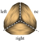
(a)

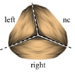
(b)

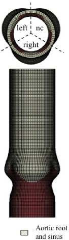
(c)

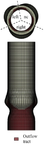
(d)

Figure 1: Geometrically idealized model of the aortic root. We use Peskin and McQueen’s theoretical model of the collagen fiber architecture of aortic valve leaflets peskin1994 to determine the shape of the leaflets for (1(a)) a symmetric and (1(b)) an asymmetric aortic valve. We use measurements of human aortic roots swanson1974 ; reul1990 to determine the geometry of the outflow tract, the sinuses, and the ascending aorta. Panel (1(c)) shows a side view and a top view of the symmetric aortic root model, and panel (1(d)) shows a side view and a top view of the asymmetric aortic root model.

2.2.2 Mechanical response

The mechanical behavior of the leaflets is described by a strain-energy functional $E=E[\bm{\mathrm{\phi}}(\cdot,t)]$ described previously griffith2009 ; griffith2012 . Briefly, let the curvilinear coordinates $\bm{\mathrm{q}}=(q,r)$ be chosen so that a fixed value of $q$ labels an individual fiber, and so that $r$ runs along the fibers. Consequently, $(\partial\bm{\mathrm{\phi}}/\partial r)/\|\partial\bm{\mathrm{\phi}}/\partial r\|$ is the unit fiber tangent vector. The total elastic energy $E$ is the sum of a stretching energy $E_{\text{s}}$ and a bending energy $E_{\text{b}}$,

$$E =E_{\text{s}}+E_{\text{b}},$$ (13)

$$E_{\text{s}} =\int_{U}\mathcal{E}_{\text{s}}\left(\left|\frac{\partial\bm{\mathrm{\phi}}}{\partial r}\right|;\bm{\mathrm{q}}\right)\mbox{d}\bm{\mathrm{q}},$$ (14)

$$E_{\text{b}} =\frac{1}{2}\int_{U}c_{\text{b}}(\bm{\mathrm{q}})\left|\frac{\partial^{2}\bm{\mathrm{\phi}}}{\partial r^{2}}-\frac{\partial^{2}\bar{\bm{\mathrm{\phi}}}}{\partial r^{2}}\right|^{2}\mbox{d}\bm{\mathrm{q}}.$$ (15)

Eq. (14) accounts for the total stretching energy associated with the fibers, in which $\mathcal{E}_{\text{s}}$ is a spatially inhomogeneous local stretching energy with a quadratic length-tension relationship, and eq. (15) accounts for the total bending energy associated with the fibers, in which $c_{\text{b}}$ is a spatially inhomogeneous bending stiffness and $\bar{\bm{\mathrm{\phi}}}$ is the reference configuration, which is taken to be the initial configuration. Because the valve leaflets are modeled as thin elastic surfaces, the bending resistant energy allows the model to account for the thickness of the real valve leaflets. Larger values of $c_{\text{b}}$ model a thick, stenotic valve, whereas smaller values of $c_{\text{b}}$ model a thin, flexible valve. The resulting Lagrangian body force density is the Fréchet derivative of $E$.

Valve leaflet parameters are empirically determined for a fixed leaflet discretization by choosing the leaflet stiffness so that the leaflet supports a diastolic load of approximately 80 mmHg with 10% strain in the family of fibers running from commissure to commissure. This leads to a commissural fiber stiffness of 7.5e6 dyne$/$cm. We further assume that these commissural fibers are a factor of 10 stiffer than the radial fibers that run orthogonal to the commissural fibers Sauren81 . The bending stiffness is chosen to be approximately the smallest value that yields valve leaflets that successfully coapt at the end of systole. These material parameters are chosen only to yield a functional valve, and are not represented as corresponding to those of an actual valve cusp. Nonetheless, this model of the valve leaflets does account for key structures of actual valve cusps, including the prominent fibers that run from commissure to commissure and the 10-to-1 anisotropy of real valve leaflets Sauren81 . See refs. griffith2009 and griffith2012 for further details. In preliminary studies, a sensitivity analysis was conducted for the bending stiffness of the aortic leaflets, and it was found that variations on the order of $\pm$ 25% in the bending stiffness have little effect on the physiological predictions of the models (not shown).

2.3 Aortic Wall

2.3.1 Geometry

An idealized model of the aortic root is constructed, as in previous work griffith2009 ; griffith2012 . The dimensions of this model are based on measurements by Swanson and Clark swanson1974 of human aortic roots collected at autopsy, and the geometry of the model is based on measurements by Reul et al. reul1990 from angiograms. The diameter of the aortic portion of the model is 3 cm, whereas the diameter of the sinus region, measured from a commissura to the center of a sinus, is 3.5 cm. The overall length of the model is of 10 cm, and the distance between the annulus and the aortic flow outlet is 7.75 cm. The thickness is constant throughout the model and is 2 mm shunk2001 . In our simulations, we employ a semi-rigid model of the left-ventricular outflow tract while allowing for a fully flexible description of the aortic sinuses and the ascending aorta. The aortic annulus, which is the scalloped line of attachment between the valve leaflets and the aortic sinuses, was considered to be the lower boundary of the sinuses; see fig. 1. The aortic model used in this study differs from previous work griffith2009 ; griffith2012 in that here we treat the aortic sinuses and ascending aorta as an incompressible hyperelastic material, whereas in earlier studies it was treated as a rigid structure.

In our simulations, we consider both symmetric and asymmetric models of the aortic root. In the symmetric model, we assume that the initial and reference configurations of the aortic root exhibit three-fold symmetry, so that each sinus and the corresponding leaflet occupies an angle of 120^∘. For the asymmetric model, the symmetric geometry is modified so that each sinus, along with the corresponding leaflet, covers a different angle. Based on the work of Berdajs berdajs2002 , the average angle covered by each leaflet was found to be $136.22^{\circ}$ for the right coronary sinus, $122.48^{\circ}$ for the noncoronary sinus, and $101.3^{\circ}$ for the left coronary sinus. Other characteristic dimensions of the leaflets, such as the radius or the height of the coapting region, were taken to be the same as the symmetric model; see fig. 1.

Because the geometry of the valve leaflets are defined in a closed and loaded configuration, it is also necessary to specify the geometry of the vessel wall in a loaded configuration, and to compute the corresponding unloaded configuration. This configuration will depend on both the prescribed loaded configuration and the constitutive model. To determine the unloaded configuration, we employ an iterative method described by Bols et al. bols2012 detailed in sec. 2.5.4.

2.3.2 Mechanical response

We describe the elasticity of the aortic sinuses and ascending aorta using a hyperelastic constitutive model fit to biaxial tensile test data collected by Azadani et al. azadani2012 from tissue samples from human aortic sinuses. Because the data reported by Azadani et al. indicate a nearly isotropic material response (see fig. 2), in this work we model the material response of the aortic sinuses and ascending aorta using an isotropic strain-energy functional $W$ with an exponential stress-strain relation,

$$W=\frac{c}{2b}\left[\exp(b(I_{1}-3))-1\right],$$ (16)

in which $I_{1}=I_{1}(\mathbb{C})=\mathop{\mathrm{tr}}(\mathbb{C})$ is the first invariant of the right Cauchy-Green strain tensor $\mathbb{C}=\mathbb{F}^{T}\mathbb{F}$, and $\mathbb{F}=\partial\bm{\mathrm{\chi}}/\partial\bm{\mathrm{X}}$ is the deformation gradient tensor associated with the deformation mapping $\bm{\mathrm{\chi}}:(V,t)\mapsto\Omega$. Material parameters were obtained by least-squares fits to experimental data using MATLAB (Mathworks, Inc., Natick, MA, USA). The first Piola-Kirchhoff stress tensor $\mathbb{P}$ is determined from $W$ via

$$\mathbb{P}=\frac{\partial W}{\partial\mathbb{F}}-p_{\text{s}}\,\mathbb{F}^{-T}=c\exp(b(I_{1}-3))\,\mathbb{F}-p_{\text{s}}\,\mathbb{F}^{-T},$$ (17)

in which $p_{\text{s}}$ is a structural pressure-like term that is chosen to improve the accuracy of the stress predictions of the method HGao14-iblv_diastole . As in earlier work HGao14-iblv_diastole , we compute $p_{\text{s}}$ via

$$p_{\text{s}}=c\exp(b(I_{1}-3))-\beta_{\text{s}}\log(I_{3}),$$ (18)

in which $I_{3}=I_{3}(\mathbb{C})=\det(\mathbb{C})$ is the third invariant of $\mathbb{C}$ and $\beta_{\text{s}}=\text{2.5e4}~{}\text{kPa}$. Thus, $\mathbb{P}=\bm{\mathrm{0}}$ for $\mathbb{F}=\mathbb{I}$, and the structural model provides an energetic penalty for any compressible deformations.

2.4 Driving and Loading Conditions

A left-ventricular pressure waveform adapted from human clinical data of Murgo et al. murgo1980 is prescribed at the upstream inlet of the left-ventricular outflow tract to drive flow through the model aortic root, and downstream loading conditions are provided by a three-element Windkessel model by Stergiopolus et al. stergiopulos1999 fit to the clinical data of Murgo et al. murgo1980 . As in earlier work griffith2009 ; griffith2012 , zero pressure boundary conditions are imposed on the boundary of the fluid-filled region exterior to the aortic root model. Coupling between the detailed IB model and the reduced circulation models is also done as in earlier work griffith2009 ; griffith2012 .

2.5 Numerical Methods

We use a locally-refined staggered-grid discretization of the Eulerian equations along with a finite difference-based discretization of the fiber model of the valve leaflets and a finite element-based description of the continuum vessel wall model. Our approach is similar to the spatially adaptive IB scheme described previously griffith2012 , except that here we also employ a finite element-based description of the aortic wall, using an approach introduced by Griffith and Luo griffith-submitted .

2.5.1 Eulerian and Lagrangian spatial discretizations

The physical domain $\Omega$ is discretized using a locally-refined Cartesian grid, but for simplicity we describe only the uniform-grid version of this method; details on the adaptively refined discretization are provided by ref. griffith2012 . Let $(i,j,k)$ index the Cartesian grid cells, and let $\bm{\mathrm{x}}_{i,j,k}=(\mbox{$(i+\frac{1}{2})$}h,\mbox{$(j+\frac{1}{2})$}h,\mbox{$(k+\frac{1}{2})$}h)$ indicate the position of the center of grid cell $(i,j,k)$, in which $h$ is the Cartesian grid meshwidth and $\Delta\bm{\mathrm{x}}=h^{3}$ is the Cartesian grid cell volume. The Eulerian velocity field $\bm{\mathrm{u}}=(u,v,w)$ is approximated at the center of each face of the Cartesian grid cells in terms of the velocity component that is normal to that face: $u$ is approximated at the locations $\bm{\mathrm{x}}_{i-\frac{1}{2},j,k}$; $v$ is approximated at the locations $\bm{\mathrm{x}}_{i,j-\frac{1}{2},k}$; and $w$ is approximated at $\bm{\mathrm{x}}_{i,j,k-\frac{1}{2}}$. The Eulerian force densities $\bm{\mathrm{f}}$ and $\bm{\mathrm{g}}$ are approximated in the same staggered-grid fashion. The Eulerian pressure $p$ is approximated at the centers of the Cartesian grid cells.

The deformations and forces associated with the valve leaflets are approximated on a fiber-aligned curvilinear mesh. Let $l$ index the nodes of this mesh, let $\bm{\mathrm{\phi}}_{l}$ and $\bm{\mathrm{F}}_{l}$ indicate the current position and Lagrangian force density of node $l$, respectively, and let $\Delta\bm{\mathrm{q}}_{l}$ indicate the area fraction (quadrature weight) associated with node $l$. $\bm{\mathrm{F}}_{l}$ is computed from $\bm{\mathrm{\phi}}_{l}$ using a finite difference approximation to the fiber force density; see refs. griffith2009 and griffith2012 for details, including relevant finite difference formulae.

The deformations, stresses, and resultant forces associated with the aortic wall are approximated on a volumetric Lagrangian mesh. Let $e$ index the elements of this mesh, with $V_{e}$ indicating the volume associated with element $e$, so that $V=\cup_{e}V_{e}$, let $m$ index the mesh nodes, and let $\varphi_{m}(\bm{\mathrm{X}})$ indicate the interpolatory Lagrangian finite element basis function associated with node $m$. The structural deformation and elastic force density are approximated in a standard manner via

$$\bm{\mathrm{\chi}}(\bm{\mathrm{X}},t) =\sum_{m}\bm{\mathrm{\chi}}_{m}(t)\,\varphi_{m}(\bm{\mathrm{X}})$$ (19)

$$\bm{\mathrm{G}}(\bm{\mathrm{X}},t) =\sum_{m}\bm{\mathrm{G}}_{m}(t)\,\varphi_{m}(\bm{\mathrm{X}}),$$ (20)

in which $\bm{\mathrm{\chi}}_{m}(t)$ are the nodal positions and $\bm{\mathrm{G}}_{m}(t)$ are the nodal force densities. The deformation gradient $\mathbb{F}$ is computed by directly differentiating the approximation to $\bm{\mathrm{\chi}}(\bm{\mathrm{X}},t)$, and $\mathbb{P}$ is evaluated from the approximation to $\mathbb{F}$. The nodal values $\bm{\mathrm{G}}_{m}(t)$ are determined so that

$$\int_{V}\bm{\mathrm{G}}(\bm{\mathrm{X}},t)\,\varphi_{n}(\bm{\mathrm{X}})\,\mbox{d}\bm{\mathrm{X}}=-\int_{V}\mathbb{P}(\bm{\mathrm{X}},t)\,\nabla_{\bm{\mathrm{X}}}\varphi_{n}(\bm{\mathrm{X}})\,\mbox{d}\bm{\mathrm{X}}$$ (21)

for all $n$. This leads to a linear system of equations that defines the nodal force densities in terms of the nodal deformations. In practice, these integrals are evaluated element-by-element using Gaussian quadrature rules that are exact for the left-hand side but are generally only approximate for the right-hand side.

2.5.2 Lagrangian-Eulerian interaction

To couple the Lagrangian and Eulerian discretizations, we employ approximations to the integral transforms of the continuum equations that replace the singular Dirac delta function $\delta(\bm{\mathrm{x}})=\mbox{$\delta(x)\,\delta(y)\,\delta(z)$}$ by a regularized delta function $\delta_{h}(\bm{\mathrm{x}})=\mbox{$\delta_{h}(x)\,\delta_{h}(y)\,\delta_{h}(z)$}$. In our computations, we construct the three-dimensional regularized delta function either by using the four-point one-dimensional regularized delta function of Peskin peskin2002 , or by using a broadened version of this function that has a spatial extent of 8 meshwidths. The same regularized delta function is used for both the thin model of the valve leaflets and the volumetric model of the vessel wall.

For the leaflet model, we employ a coupling approach frequently used with the IB method. The Lagrangian forces $\bm{\mathrm{F}}=(F^{x},F^{y},F^{z})$ associated with the leaflets are converted into equivalent Eulerian forces $\bm{\mathrm{f}}=(f^{x},f^{y},f^{z})$ via

$$f^{x}_{i-\frac{1}{2},j,k} =\sum_{l}F_{l}^{x}\,\delta_{h}(\bm{\mathrm{x}}_{i-\frac{1}{2},j,k}-\bm{\mathrm{\phi}}_{l})\,\Delta\bm{\mathrm{q}}_{l},$$ (22)

$$f^{y}_{i,j-\frac{1}{2},k} =\sum_{l}F_{l}^{y}\,\delta_{h}(\bm{\mathrm{x}}_{i,j-\frac{1}{2},k}-\bm{\mathrm{\phi}}_{l})\,\Delta\bm{\mathrm{q}}_{l},$$ (23)

$$f^{z}_{i,j,k-\frac{1}{2}} =\sum_{l}F_{l}^{z}\,\delta_{h}(\bm{\mathrm{x}}_{i,j,k-\frac{1}{2}}-\bm{\mathrm{\phi}}_{l})\,\Delta\bm{\mathrm{q}}_{l}.$$ (24)

This amounts to using the trapezoidal rule to discretize the integral transform (3). We employ the compact notation

$$\bm{\mathrm{f}}=\bm{\mathrm{\mathcal{S}}}^{\text{l}}[\bm{\mathrm{\phi}}]\,\bm{\mathrm{F}}$$ (25)

to express this force-spreading operation. The Eulerian velocity $\bm{\mathrm{u}}=(u,v,w)$ is used to determine the dynamics of the physical positions $\bm{\mathrm{\phi}}=(\phi^{x},\phi^{y},\phi^{z})$ of the material points of the valve leaflets via

$$\frac{\mathrm{d}}{\mathrm{d}t}\phi_{l}^{x} =\sum_{i,j,k}u_{i-\frac{1}{2},j,k}\,\delta_{h}(\bm{\mathrm{x}}_{i-\frac{1}{2},j,k}-\bm{\mathrm{\phi}}_{l})\,\Delta\bm{\mathrm{x}},$$ (26)

$$\frac{\mathrm{d}}{\mathrm{d}t}\phi_{l}^{y} =\sum_{i,j,k}v_{i,j-\frac{1}{2},k}\,\delta_{h}(\bm{\mathrm{x}}_{i,j-\frac{1}{2},k}-\bm{\mathrm{\phi}}_{l})\,\Delta\bm{\mathrm{x}},$$ (27)

$$\frac{\mathrm{d}}{\mathrm{d}t}\phi_{l}^{z} =\sum_{i,j,k}w_{i,j,k-\frac{1}{2}}\,\delta_{h}(\bm{\mathrm{x}}_{i,j,k-\frac{1}{2}}-\bm{\mathrm{\phi}}_{l})\,\Delta\bm{\mathrm{x}}.$$ (28)

We use the notation

$$\frac{\mathrm{d}}{\mathrm{d}t}\bm{\mathrm{\phi}}=\bm{\mathrm{\mathcal{R}}}^{\text{l}}[\bm{\mathrm{\phi}}]\,\bm{\mathrm{u}}$$ (29)

to express this velocity-restriction operation. Notice that by construction, the force-spreading and velocity-interpolation operators are adjoints, i.e., $\bm{\mathrm{\mathcal{R}}}^{\text{l}}[\bm{\mathrm{\phi}}]=\bm{\mathrm{\mathcal{S}}}^{\text{l}}[\bm{\mathrm{\phi}}]^{*}$.

The Lagrangian-Eulerian coupling scheme used for the vessel model is based on an approach developed by Griffith and Luo griffith-submitted . This approach is first to construct a force-spreading operator, and then to determine a velocity-restriction operator that is the adjoint of the force-spreading operator. Briefly, for each element $e$, a set of quadrature points $Q(e)$ is determined, and for each quadrature point $q\in Q(e)$, $\bm{\mathrm{X}}_{q}^{e}$ indicates the reference coordinates of the quadrature point, and $\omega_{q}^{e}$ indicates the quadrature weight associated. The Lagrangian force density $\bm{\mathrm{G}}=(G^{x},G^{y},G^{z})$ is converted into the equivalent Eulerian force density $\bm{\mathrm{g}}=(g^{x},g^{y},g^{z})$ by discretizing eq. (9), with $\delta(\bm{\mathrm{x}})$ replaced by $\delta_{h}(\bm{\mathrm{x}})$, using this quadrature rule, i.e.

$$g^{x}_{i-\frac{1}{2},j,k} =\sum_{e}\sum_{q\in Q(e)}G^{x}(\bm{\mathrm{X}}_{q}^{e},t)\,\delta_{h}(\bm{\mathrm{x}}_{i-\frac{1}{2},j,k}-\bm{\mathrm{\chi}}(\bm{\mathrm{X}}_{q}^{e},t))\,\omega_{q}^{e},$$ (30)

$$g^{y}_{i,j-\frac{1}{2},k} =\sum_{e}\sum_{q\in Q(e)}G^{y}(\bm{\mathrm{X}}_{q}^{e},t)\,\delta_{h}(\bm{\mathrm{x}}_{i,j-\frac{1}{2},k}-\bm{\mathrm{\chi}}(\bm{\mathrm{X}}_{q}^{e},t))\,\omega_{q}^{e},$$ (31)

$$g^{z}_{i,j,k-\frac{1}{2}} =\sum_{e}\sum_{q\in Q(e)}G^{z}(\bm{\mathrm{X}}_{q}^{e},t)\,\delta_{h}(\bm{\mathrm{x}}_{i,j,k-\frac{1}{2}}-\bm{\mathrm{\chi}}(\bm{\mathrm{X}}_{q}^{e},t))\,\omega_{q}^{e}.$$ (32)

Notice that these formulae take advantage of the fact that we may evaluate the approximations to $\bm{\mathrm{G}}$ and $\bm{\mathrm{\chi}}$ at arbitrary Lagrangian locations. Specifically, we are not restricted to evaluating $\bm{\mathrm{G}}$ and $\bm{\mathrm{\chi}}$ at the nodes of the finite element mesh. In practice, the quadrature rules are dynamically determined to ensure that the physical spacing of the quadrature points is on average one-half of a Cartesian meshwidth, even under the presence of extremely large structural deformations. We use the notation

$$\bm{\mathrm{g}}=\bm{\mathrm{\mathcal{S}}}^{\text{w}}[\bm{\mathrm{\chi}}]\,\bm{\mathrm{G}}$$ (33)

to denote the force-spreading operator.

To determine the corresponding velocity-restriction operator, we introduce a Lagrangian velocity field $\bm{\mathrm{U}}=(U,V,W)$, which is defined in terms of nodal velocities $\bm{\mathrm{U}}_{m}$ via

$$\bm{\mathrm{U}}(\bm{\mathrm{X}},t)=\sum_{m}\bm{\mathrm{U}}_{m}(t)\,\varphi_{m}(\bm{\mathrm{X}}).$$ (34)

This velocity field is required to satisfy, for all $n$,

$$\sum_{e}\sum_{q\in Q(e)}U(\bm{\mathrm{X}}_{q}^{e},t)\,\varphi_{n}(\bm{\mathrm{X}}_{q}^{e})\,\omega_{q}^{e}$$

$$\mbox{}\hskip 54.2025pt=\sum_{e}\sum_{q\in Q(e)}\left(\sum_{i,j,k}u_{i-\frac{1}{2},j,k}\delta_{h}(\bm{\mathrm{x}}_{i-\frac{1}{2},j,k}-\bm{\mathrm{\chi}}(\bm{\mathrm{X}}_{q}^{e},t))\,\Delta\bm{\mathrm{x}}\right)\varphi_{n}(\bm{\mathrm{X}}_{q}^{e})\,\omega_{q}^{e},$$ (35)

$$\sum_{e}\sum_{q\in Q(e)}V(\bm{\mathrm{X}}_{q}^{e},t)\,\varphi_{n}(\bm{\mathrm{X}}_{q}^{e})\,\omega_{q}^{e}$$

$$\mbox{}\hskip 54.2025pt=\sum_{e}\sum_{q\in Q(e)}\left(\sum_{i,j,k}v_{i,j-\frac{1}{2},k}\delta_{h}(\bm{\mathrm{x}}_{i,j-\frac{1}{2},k}-\bm{\mathrm{\chi}}(\bm{\mathrm{X}}_{q}^{e},t))\,\Delta\bm{\mathrm{x}}\right)\varphi_{n}(\bm{\mathrm{X}}_{q}^{e})\,\omega_{q}^{e},$$ (36)

$$\sum_{e}\sum_{q\in Q(e)}W(\bm{\mathrm{X}}_{q}^{e},t)\,\varphi_{n}(\bm{\mathrm{X}}_{q}^{e})\,\omega_{q}^{e}$$

$$\mbox{}\hskip 54.2025pt=\sum_{e}\sum_{q\in Q(e)}\left(\sum_{i,j,k}w_{i,j,k-\frac{1}{2}}\delta_{h}(\bm{\mathrm{x}}_{i,j,k-\frac{1}{2}}-\bm{\mathrm{\chi}}(\bm{\mathrm{X}}_{q}^{e},t))\,\Delta\bm{\mathrm{x}}\right)\varphi_{n}(\bm{\mathrm{X}}_{q}^{e})\,\omega_{q}^{e}.$$ (37)

This yields a system of linear equations to be solved for the nodal values of $\bm{\mathrm{U}}$. Notice that eqs. (35)–(37) correspond to a discrete component-wise approximation to eq. (12). We use the notation

$$\frac{\mathrm{d}}{\mathrm{d}t}\bm{\mathrm{\chi}}=\bm{\mathrm{U}}=\bm{\mathrm{\mathcal{R}}}^{\text{w}}[\bm{\mathrm{\chi}}]\,\bm{\mathrm{u}}.$$ (38)

Notice that $\bm{\mathrm{\mathcal{R}}}^{\text{w}}[\bm{\mathrm{\chi}}]$ is a nonlocal operator in the sense that it requires the solution of a system of linear equations. Although not shown here, it is the case that $\bm{\mathrm{\mathcal{R}}}^{\text{w}}[\bm{\mathrm{\chi}}]=\bm{\mathrm{\mathcal{S}}}^{\text{w}}[\bm{\mathrm{\chi}}]^{*}$. See Griffith and Luo griffith-submitted for further discussion.

2.5.3 Time stepping

The time stepping scheme is similar to that of Griffith and Luo griffith-submitted . Let $\Delta t$ indicate the (uniform) time step size, and let $[t^{n},t^{n+1}]=[n\Delta t,(n+1)\Delta t]$ indicate the $n^{\text{th}}$ time interval. In this subsection, superscript indices always indicate the time step number. The state variables $\bm{\mathrm{u}}$, $\bm{\mathrm{\phi}}$, and $\bm{\mathrm{\chi}}$ are defined at integer time steps. The pressure $p$, which is not a state variable of the system, is defined at half-integer time steps. Approximations to the state variables and to derived quantities such as the Lagrangian forces are also evaluated at half-integer time steps.

The time stepping scheme proceeds as follows. First, predicted intermediate approximations to the structural deformations $\bm{\mathrm{\phi}}$ and $\bm{\mathrm{\chi}}$ at time $t^{n+\frac{1}{2}}$ are determined via

$$\frac{\bm{\mathrm{\phi}}^{n+\frac{1}{2}}-\bm{\mathrm{\phi}}^{n}}{\Delta t/2} =\bm{\mathrm{\mathcal{R}}}^{\text{l}}[\bm{\mathrm{\phi}}^{n}]\bm{\mathrm{u}}^{n},$$ (39)

$$\frac{\bm{\mathrm{\chi}}^{n+\frac{1}{2}}-\bm{\mathrm{\chi}}^{n}}{\Delta t/2} =\bm{\mathrm{\mathcal{R}}}^{\text{w}}[\bm{\mathrm{\chi}}^{n}]\bm{\mathrm{u}}^{n}.$$ (40)

This is an application of the forward Euler time stepping scheme. Lagrangian force densities $\bm{\mathrm{F}}^{n+\frac{1}{2}}$ and $\bm{\mathrm{G}}^{n+\frac{1}{2}}$ are determined from the predicted structure configurations, and these Lagrangian force densities are spread to the Cartesian grid via

$$\bm{\mathrm{f}}^{n+\frac{1}{2}} =\bm{\mathrm{\mathcal{S}}}^{\text{l}}[\bm{\mathrm{\phi}}^{n+\frac{1}{2}}]\bm{\mathrm{F}}^{n+\frac{1}{2}},$$ (41)

$$\bm{\mathrm{g}}^{n+\frac{1}{2}} =\bm{\mathrm{\mathcal{S}}}^{\text{w}}[\bm{\mathrm{\chi}}^{n+\frac{1}{2}}]\bm{\mathrm{G}}^{n+\frac{1}{2}}.$$ (42)

Next, we solve the discretized incompressible Navier-Stokes equations for $\bm{\mathrm{u}}^{n+1}$ and $p^{n+\frac{1}{2}}$ via a Crank-Nicolson Adams-Bashforth scheme,

$$\rho\left(\frac{\bm{\mathrm{u}}^{n+1}-\bm{\mathrm{u}}^{n}}{\Delta t}+\left[\bm{\mathrm{u}}\cdot\nabla_{h}\bm{\mathrm{u}}\right]^{(n+\frac{1}{2})}\right) =-\nabla_{h}p^{n+\frac{1}{2}}+\mu\nabla_{h}^{2}\left(\frac{\bm{\mathrm{u}}^{n+1}+\bm{\mathrm{u}}^{n}}{2}\right)$$

$$\ \ \ \ \ \ \ \ \ \ \mbox{}+\bm{\mathrm{f}}^{n+\frac{1}{2}}+\bm{\mathrm{g}}^{n+\frac{1}{2}},$$ (43)

$$\nabla_{h}\cdot\bm{\mathrm{u}}^{n+1} =0,$$ (44)

with

$$\left[\bm{\mathrm{u}}\cdot\nabla_{h}\bm{\mathrm{u}}\right]^{(n+\frac{1}{2})}=\frac{3}{2}\bm{\mathrm{u}}^{n}\cdot\nabla_{h}\bm{\mathrm{u}}^{n}-\frac{1}{2}\bm{\mathrm{u}}^{n-1}\cdot\nabla_{h}\bm{\mathrm{u}}^{n-1}.$$ (45)

In the uniform grid case, the discrete operators $\nabla_{h}$, $\nabla_{h}\cdot\mbox{}$, and $\nabla_{h}^{2}$ are standard second-order accurate staggered-grid finite difference approximations to the gradient, divergence, and Laplace operators, respectively griffith2009-efficient . We compute $\bm{\mathrm{u}}\cdot\nabla_{h}\bm{\mathrm{u}}$ via a staggered-grid version of the piecewise parabolic method (PPM) griffith2009-efficient . On locally-refined Cartesian grids, these discrete operators are straightforward extensions of the uniform grid operators griffith2012 . Solving eqs. (43) and (44) for $\bm{\mathrm{u}}^{n+1}$ and $p^{n+\frac{1}{2}}$ requires the solution of the time-dependent Stokes equations. The Stokes equations are solved using an iterative Krylov method with a multigrid preconditioner derived from the classical projection method griffith2009-efficient ; cai-submitted .

Finally, we determine approximations to the structural deformations at the end of the time step via

$$\frac{\bm{\mathrm{\phi}}^{n+1}-\bm{\mathrm{\phi}}^{n}}{\Delta t} =\bm{\mathrm{\mathcal{R}}}^{\text{l}}[\bm{\mathrm{\phi}}^{n+\frac{1}{2}}]\bm{\mathrm{u}}^{n+\frac{1}{2}},$$ (46)

$$\frac{\bm{\mathrm{\chi}}^{n+1}-\bm{\mathrm{\chi}}^{n}}{\Delta t} =\bm{\mathrm{\mathcal{R}}}^{\text{w}}[\bm{\mathrm{\chi}}^{n+\frac{1}{2}}]\bm{\mathrm{u}}^{n+\frac{1}{2}},$$ (47)

with

$$\bm{\mathrm{u}}^{n+\frac{1}{2}}=\frac{\bm{\mathrm{u}}^{n+1}+\bm{\mathrm{u}}^{n}}{2}.$$ (48)

This is an application of the explicit midpoint rule to the structural dynamics.

In the initial time step, we do not have a value for $\bm{\mathrm{u}}^{n-1}$ as required to evaluate the Adams-Bashforth approximation to the convective term. Consequently, in the initial time step, we employ a two-step Runge-Kutta scheme.

Within each time step, coupling between the detailed fluid-structure interaction model and the reduced Windkessel model of the circulation is done as described previously griffith2009 ; griffith2012 . In this approach, we perform only a single Stokes solve per time step, except in the initial time step, when we perform two Stokes solves within the context of a two-step Runge-Kutta scheme.

2.5.4 Backward displacement method

To determine the unloaded configuration of the vessel wall, we use an iterative backward displacement method described by Bols et al. bols2012 implemented using a custom MATLAB script that interfaces with the ABAQUS (Dassault Systèmes Simulia Corp., Providence, RI, USA) finite element analysis software. Because the constitutive model (16) is not provided by ABAQUS, this model was implemented using a UHYPER subroutine.

Let $\bm{\mathrm{x}}_{m}$ denote positions of the finite element mesh nodes in the prescribed loaded configuration, let $\bm{\mathrm{X}}_{m}^{i}$ denote the corresponding nodal positions in the computed reference configuration after $i$ iterations of the backward displacement algorithm, and let $\bm{\mathrm{\chi}}_{m}^{i}=\bm{\mathrm{\chi}}_{m}[\bm{\mathrm{X}}^{i}]$ denote nodal positions in the computed loaded configuration when $\bm{\mathrm{X}}^{i}$ is used as the unloaded reference configuration. Notice that $\bm{\mathrm{x}}_{m}$, $\bm{\mathrm{X}}_{m}^{i}$, and $\bm{\mathrm{\chi}}_{m}^{i}$ are all defined at the nodes of the finite element mesh.

The algorithm is straightforward: First, we initialize $\bm{\mathrm{X}}^{0}:=\bm{\mathrm{x}}$ (i.e., we use the deformed coordinates as an initial guess for the unloaded configuration). Then, given $\bm{\mathrm{X}}^{i}$, $\bm{\mathrm{X}}^{i+1}$ is determined by

$$\bm{\mathrm{X}}^{i+1}:=\bm{\mathrm{X}}^{i}+(\bm{\mathrm{x}}-\bm{\mathrm{\chi}}^{i}).$$ (49)

Notice that if we define the displacement from the computed reference configuration to the deformed coordinates at step $i$ by $\bm{\mathrm{D}}^{i}=\bm{\mathrm{\chi}}^{i}-\bm{\mathrm{X}}^{i}$, then (49) is equivalent to

$$\bm{\mathrm{X}}^{i+1}:=\bm{\mathrm{x}}-\bm{\mathrm{D}}^{i}.$$ (50)

Thus, the reference coordinates are determined via a backward displacement from the deformed configuration. If this process converges, $\bm{\mathrm{\chi}}^{i}\rightarrow\bm{\mathrm{x}}$ and we obtain reference coordinates $\bm{\mathrm{X}}$ such that $\bm{\mathrm{\chi}}[\bm{\mathrm{X}}]=\bm{\mathrm{x}}$.

The convergence of this iterative process is assessed in terms of the discrete $L^{2}$ norm of the residual $\bm{\mathrm{x}}-\bm{\mathrm{\chi}}^{i}$, i.e.

$$r^{i}=\|\bm{\mathrm{x}}-\bm{\mathrm{\chi}}[\bm{\mathrm{X}}^{i}]\|_{2}=\left(\sum_{m}\|\bm{\mathrm{x}}_{m}-\bm{\mathrm{\chi}}_{m}^{i}\|_{2}^{2}\right)^{1/2}.$$ (51)

The routine was judged to have converged once the residual was less than 0.1% of the average vessel radius and the change in the residual between two consecutive iterations was less than 0.015% of the average radius. In general, obtaining convergence may require the use of damping, or of gradually increasing the loading pressure; however, in practice, we have found this algorithm to be robust, and neither damping nor incremental loading were required for the analyses performed herein.

2.5.5 Discretization

In our dynamic fluid-structure interaction simulations, the computational domain is taken to be a $10~{}\text{cm}\times 10~{}\text{cm}\times 10~{}\text{cm}$ cubic region discretized using a three-level locally refined grid. For the purposes of a mesh convergence study, two different fine grid spacings are used: a coarser one corresponding to $h=0.78125~{}\text{mm}$, which is equivalent to a uniform $128\times 128\times 128$ Eulerian discretization, and a finer one corresponding to $h=0.390625~{}\text{mm}$, which is equivalent to a uniform $256\times 256\times 256$ Eulerian discretization. The curvilinear mesh used to discretize the valve leaflets has a physical grid spacing of approximately $h/4$ for the coarser Eulerian discretization, and to $h/2$ for the finer discretization. The volumetric mesh used to discretize the vessel wall uses 23,400 8-node (trilinear) hexahedral elements for both the symmetric and the asymmetric model. The average mesh aspect ratio was $1.93\pm 0.25$ for the symmetric root model and $1.94\pm 0.34$ for the asymmetric one. A preliminary convergence study in ABAQUS was performed to ensure mesh convergence of the structural model for both the backward displacement method and the FE analysis. We use the standard four-point delta function of Peskin peskin2002 for the coarser simulations, and a broadened 8-point version of this kernel function for the higher resolution simulations, so that the physical extent of the regularized delta function is the same for both spatial resolutions. Consequently, the valve leaflets have the same effective thickness in for both spatial resolutions. A uniform time step size of $\Delta t=\text{9.94369e-6}~{}\text{s}$ was used with the coarser Eulerian discretization, whereas a uniform time step size of $\Delta t=\text{1.40625e-5}$ was used for the finer Eulerian discretization. These time step sizes are empirically determined to be within a factor of $\sqrt{2}$ of the largest time step that satisfies the stability restriction of our explicit time integration method.

3 Results

3.1 Constitutive Parameters

\psfragscanon\psfrag{s05}[t][t]{\color[rgb]{0,0,0}\begin{tabular}[]{c}Stretch\end{tabular}}\psfrag{s06}[b][b]{\color[rgb]{0,0,0}\begin{tabular}[]{c}Cauchy stress (kPa)\end{tabular}}\psfrag{s10}{\color[rgb]{0,0,0}\begin{tabular}[]{c}\end{tabular}}\psfrag{s11}{\color[rgb]{0,0,0}\begin{tabular}[]{c}\end{tabular}}\psfrag{s12}[l][l]{\color[rgb]{0,0,0}Isotropic model fit}\psfrag{s13}[l][l]{\color[rgb]{0,0,0}Axial experimental data}\psfrag{s14}[l][l]{\color[rgb]{0,0,0}Circumferential experimental data}\psfrag{s15}[l][l]{\color[rgb]{0,0,0}Isotropic model fit}\psfrag{x01}[t][t]{1}\psfrag{x02}[t][t]{1.05}\psfrag{x03}[t][t]{1.1}\psfrag{x04}[t][t]{1.15}\psfrag{x05}[t][t]{1.2}\psfrag{v01}[r][r]{0}\psfrag{v02}[r][r]{20}\psfrag{v03}[r][r]{40}\psfrag{v04}[r][r]{60}\psfrag{v05}[r][r]{80}\psfrag{v06}[r][r]{100}\psfrag{v07}[r][r]{120}\psfrag{v08}[r][r]{140}\includegraphics{Figure_2_new.eps}

Figure 2: Biaxial tensile test data obtained from human aortic root tissue samples by Azadani et al. azadani2012 and our fit of the isotropic hyperelastic constitutive model (16) to these data.

The constitutive model (16) used to describe the mechanical response of the aortic sinuses and ascending aorta is fit to data collected biaxial tensile tests of human aortic root tissue samples reported by Azadani et al. azadani2012 , yielding model parameter values of $c=12.8~{}\text{kPa}$ and $b=6.9$; see fig. 2. Recall that these material parameters are used in the aortic sinuses and ascending aorta, whereas the outflow tract is treated as an essentially rigid structure.

3.2 Unloaded Geometries

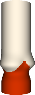
(a)

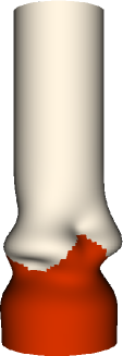
(b)

(c)

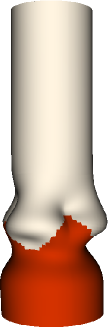
(d)

Figure 3: Views of the (3(a)) loaded and (3(b)) unloaded symmetric geometry, and of the (3(c)) loaded and (3(d)) unloaded asymmetric geometry.

\psfragscanon\psfrag{s05}[b][b]{\color[rgb]{0,0,0}\begin{tabular}[]{c}residual (m)\end{tabular}}\psfrag{s06}[t][t]{\color[rgb]{0,0,0}\begin{tabular}[]{c}iteration number\end{tabular}}\psfrag{s10}{\color[rgb]{0,0,0}\begin{tabular}[]{c}\end{tabular}}\psfrag{s11}{\color[rgb]{0,0,0}\begin{tabular}[]{c}\end{tabular}}\psfrag{s12}[l][l]{\color[rgb]{0,0,0}asymmetric model}\psfrag{s13}[l][l]{\color[rgb]{0,0,0}symmetric model}\psfrag{s14}[l][l]{\color[rgb]{0,0,0}asymmetric model}\psfrag{x01}[t][t]{0}\psfrag{x02}[t][t]{5}\psfrag{x03}[t][t]{10}\psfrag{x04}[t][t]{15}\psfrag{x05}[t][t]{20}\psfrag{x06}[t][t]{25}\psfrag{v01}[r][r]{$10^{-5}$}\psfrag{v02}[r][r]{$10^{-4}$}\psfrag{v03}[r][r]{$10^{-3}$}\psfrag{v04}[r][r]{$10^{-2}$}\includegraphics{Residuals_semilogy.eps}

Figure 4: Convergence history of the inverse displacement procedure.

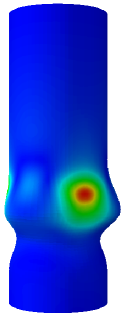
(a)

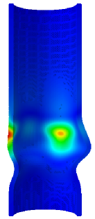
(b)

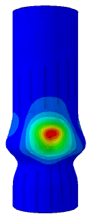
(c)

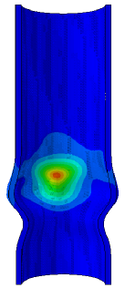
(d)

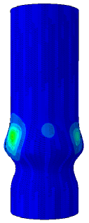
(e)

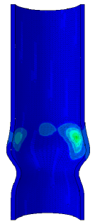
(f)

Figure 5: Contour plots showing the norm of the distance between the prescribed and computed loaded geometries. Panels (a) and (b) show the symmetric geometry, and panels (c)–(f) show the asymmetric geometry, with panels (5(c)) and (5(d)) showing the right sinus and panels (5(e)) and (5(f)) showing the left and noncoronary sinuses. Recall that the unloaded geometry is determined from the loaded geometry. The computed loaded geometry is the result of applying a prescribed pressure load to the computed unloaded geometry.

The unloaded configuration is determined by assuming that the loaded configuration corresponds to a pressure load of 80 mmHg. In fig. 3, panels (3(a)) and (3(b)) show the prescribed loaded geometry, and panels (3(c)) and (3(d)) show the computed zero-pressure configuration. Fig. 4 shows the convergence history of the backward displacement method. When the computed zero-pressure geometry is subjected to a 80 mmHg pressure load, the deformed geometry agrees with the prescribed geometry to within approximately 15 $\mu$m; see fig. 5. The discrepancy between the prescribed loaded geometry and the computed loaded geometry is greatest at the commissures and smallest along the straight portion of the vessel. Similar results are obtained for both the symmetric and asymmetric models.

3.3 Fluid-Structure Interaction Analyses

3.3.1 Symmetric model

\psfragscanon\psfrag{s05}[b][b]{\color[rgb]{0,0,0}\begin{tabular}[]{c}Pressure (mmHg)\end{tabular}}\psfrag{s06}[t][t]{\color[rgb]{0,0,0}\begin{tabular}[]{c}Time (s)\end{tabular}}\psfrag{s10}{\color[rgb]{0,0,0}\begin{tabular}[]{c}\end{tabular}}\psfrag{s11}{\color[rgb]{0,0,0}\begin{tabular}[]{c}\end{tabular}}\psfrag{s12}[l][l]{\color[rgb]{0,0,0}Left Ventricle}\psfrag{s13}[l][l]{\color[rgb]{0,0,0}Aorta N=128}\psfrag{s14}[l][l]{\color[rgb]{0,0,0}Aorta N=256}\psfrag{s15}[l][l]{\color[rgb]{0,0,0}Left Ventricle}\psfrag{x01}[t][t]{1}\psfrag{x02}[t][t]{1.5}\psfrag{x03}[t][t]{2}\psfrag{x04}[t][t]{2.5}\psfrag{x05}[t][t]{3}\psfrag{x06}[t][t]{3.5}\psfrag{x07}[t][t]{4}\psfrag{v01}[r][r]{0}\psfrag{v02}[r][r]{20}\psfrag{v03}[r][r]{40}\psfrag{v04}[r][r]{60}\psfrag{v05}[r][r]{80}\psfrag{v06}[r][r]{100}\psfrag{v07}[r][r]{120}\includegraphics{pressure.eps}

(a)

\psfragscanon\psfrag{s03}[t][t]{\color[rgb]{0,0,0}\begin{tabular}[]{c}Time (s)\end{tabular}}\psfrag{s04}[b][b]{\color[rgb]{0,0,0}\begin{tabular}[]{c}Flow Rate (ml/s)\end{tabular}}\psfrag{x01}[t][t]{1}\psfrag{x02}[t][t]{1.5}\psfrag{x03}[t][t]{2}\psfrag{x04}[t][t]{2.5}\psfrag{x05}[t][t]{3}\psfrag{x06}[t][t]{3.5}\psfrag{x07}[t][t]{4}\psfrag{v01}[r][r]{-200}\psfrag{v02}[r][r]{-100}\psfrag{v03}[r][r]{0}\psfrag{v04}[r][r]{100}\psfrag{v05}[r][r]{200}\psfrag{v06}[r][r]{300}\psfrag{v07}[r][r]{400}\psfrag{v08}[r][r]{500}\psfrag{v09}[r][r]{600}\psfrag{v10}[r][r]{700}\includegraphics{flow.eps}

(b)

Figure 6: Results of a dynamic fluid-structure interaction analysis of the symmetric aortic root over the final three simulated cardiac cycles using a coarser Cartesian grid (effective grid resolution of $N=128$) and a finer Cartesian grid (effective grid resolution of $N=256$). (6(a)) Prescribed left-ventricular driving pressure and computed aortic loading pressure, and (6(b)) computed flow rate, in which the dashed vertical lines highlight the moment that the valve leaflets open and the solid vertical lines highlight the moment that the valve leaflets close. Large oscillations indicate the reverberations of the aortic valve leaflets upon closure.

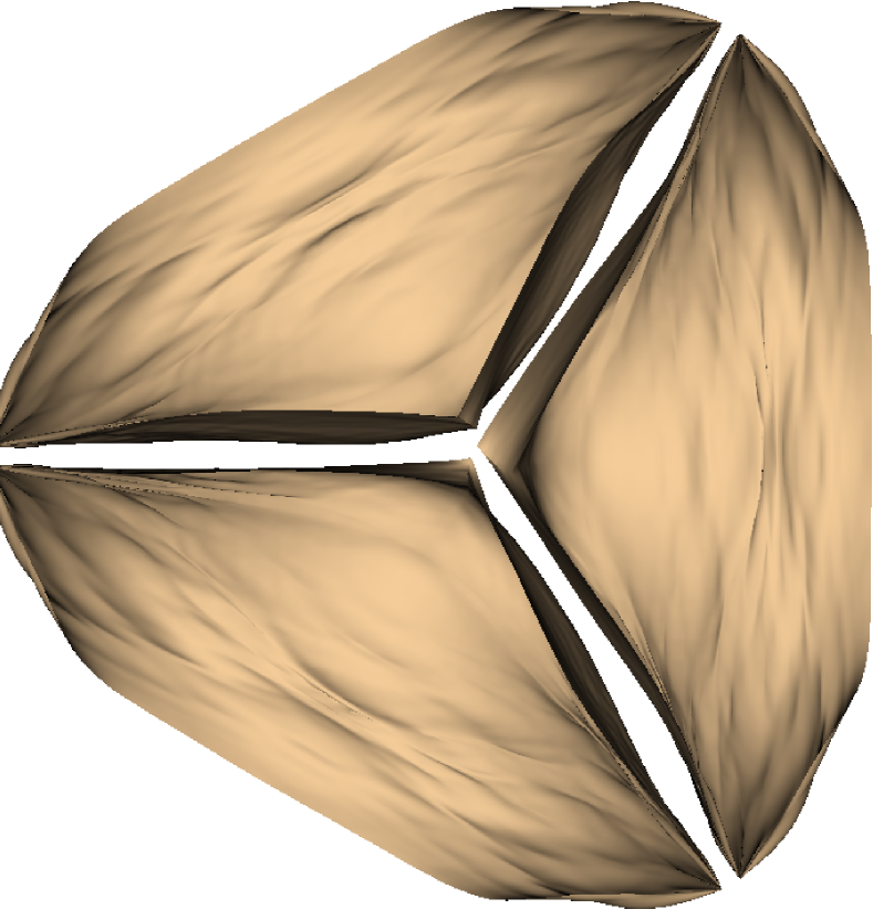
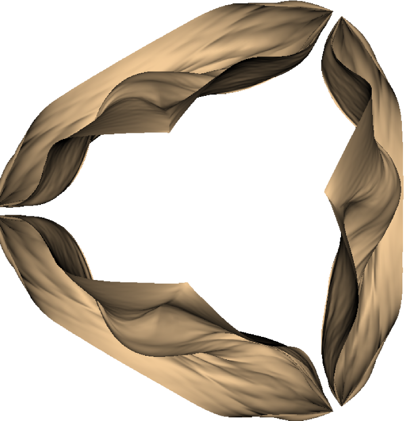
(a)

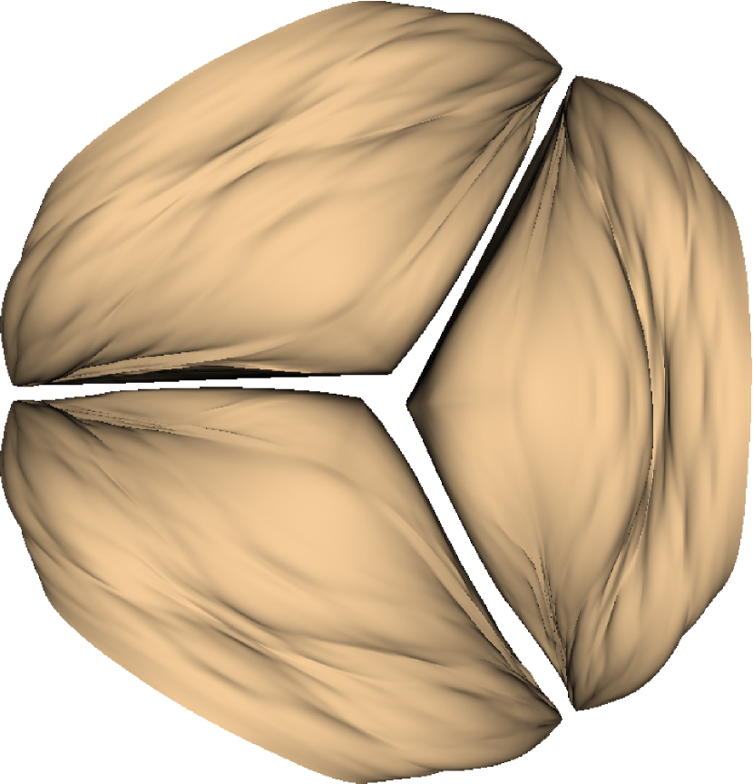
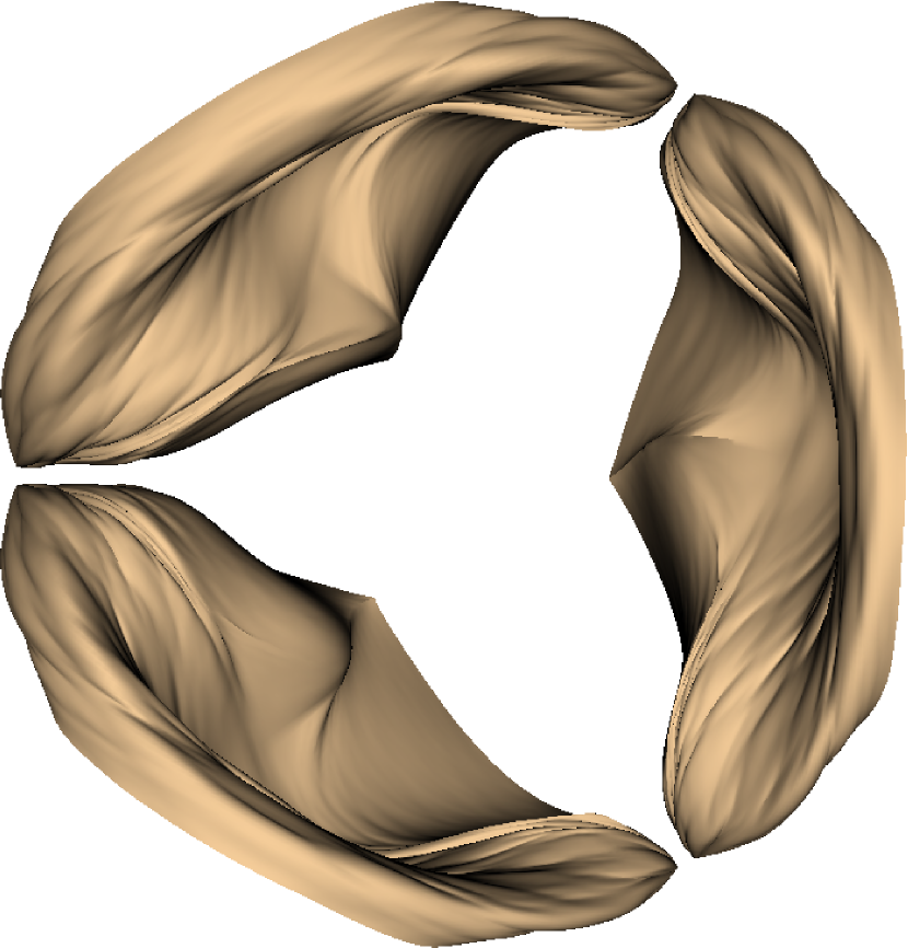
(b)

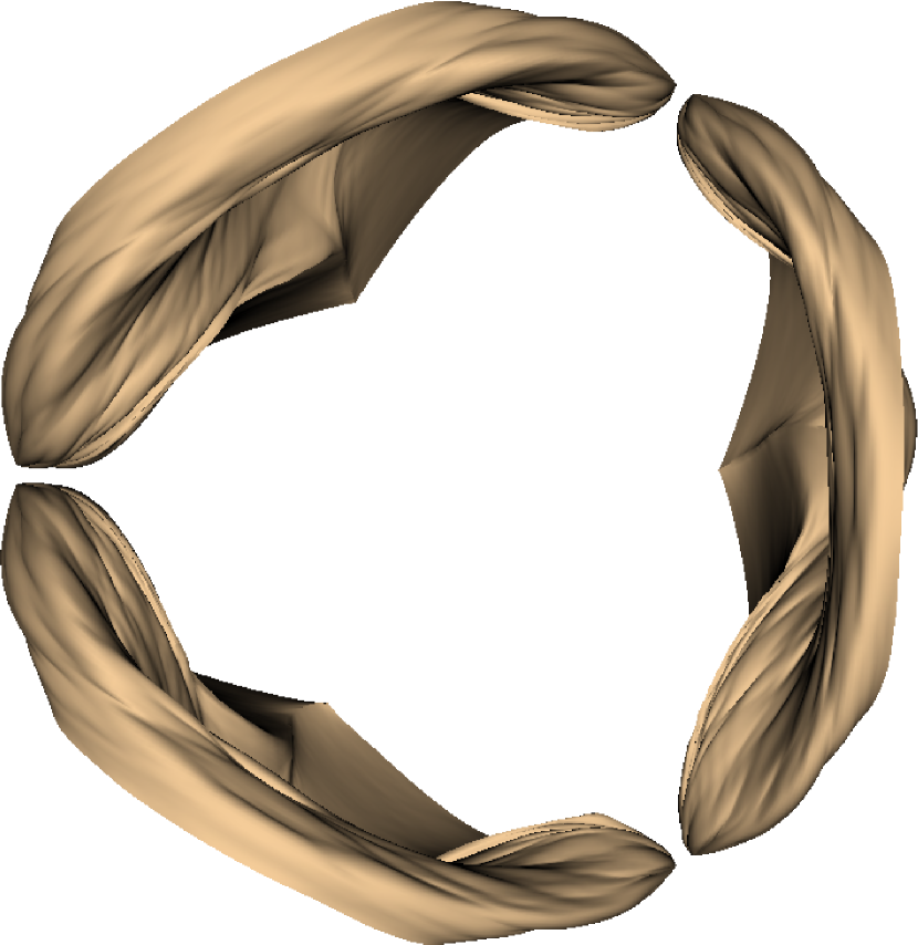
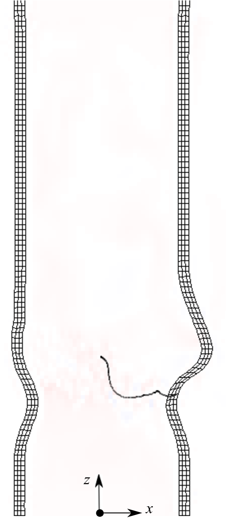
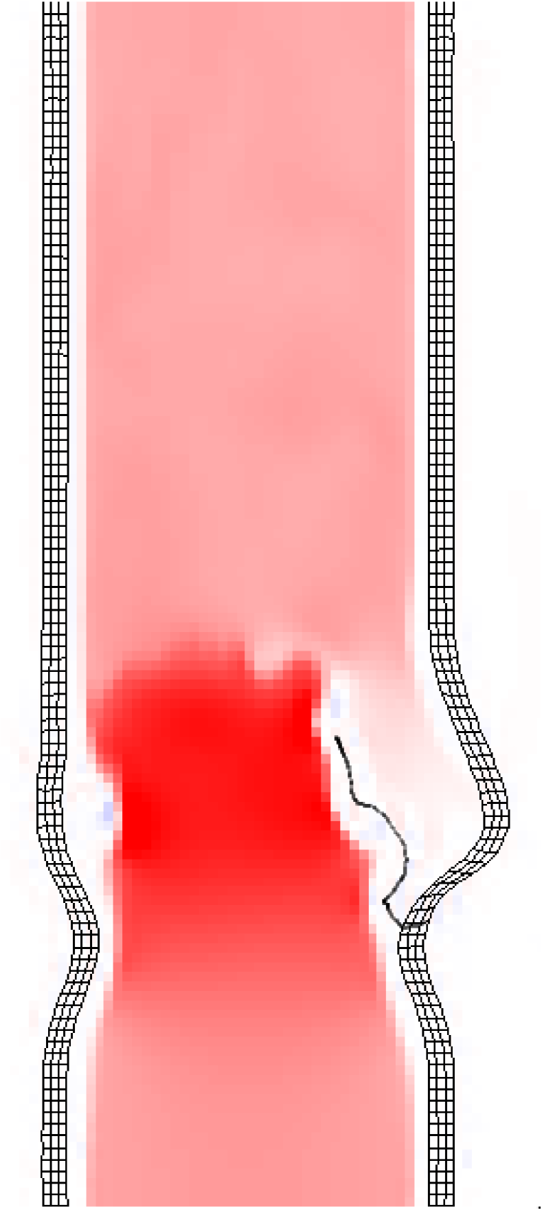
(c)

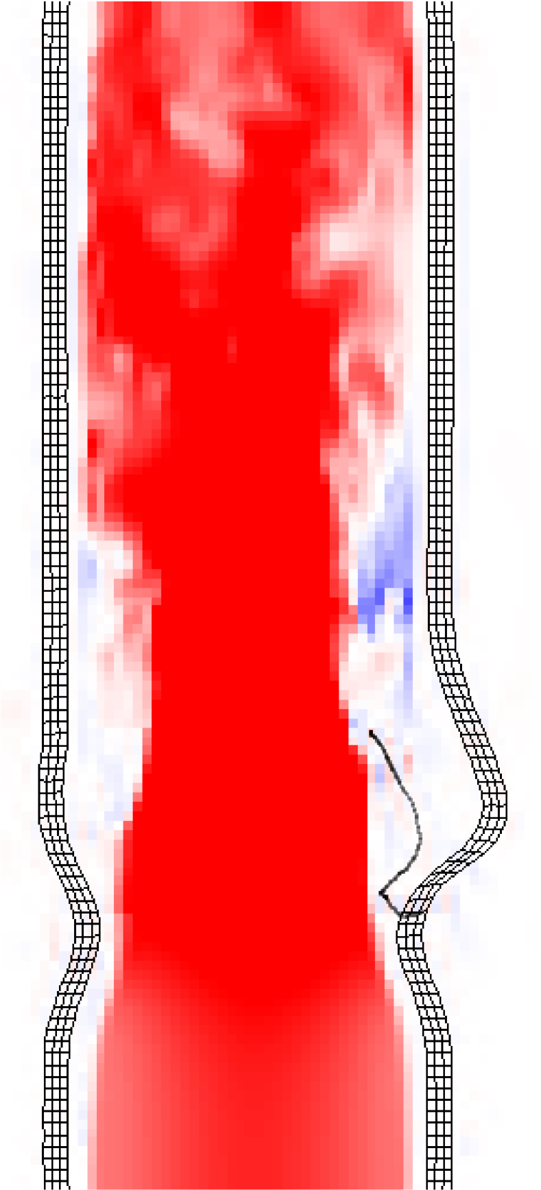
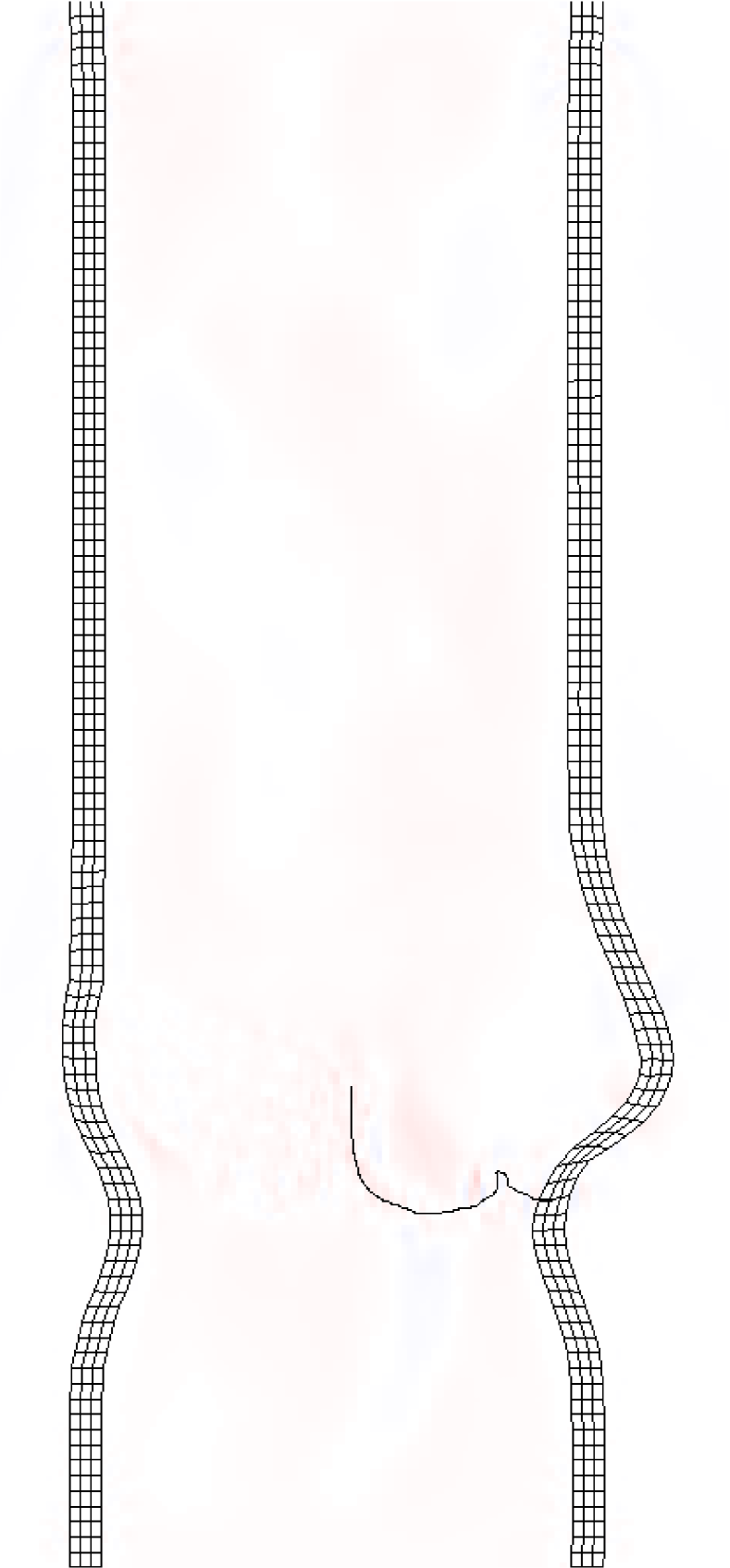
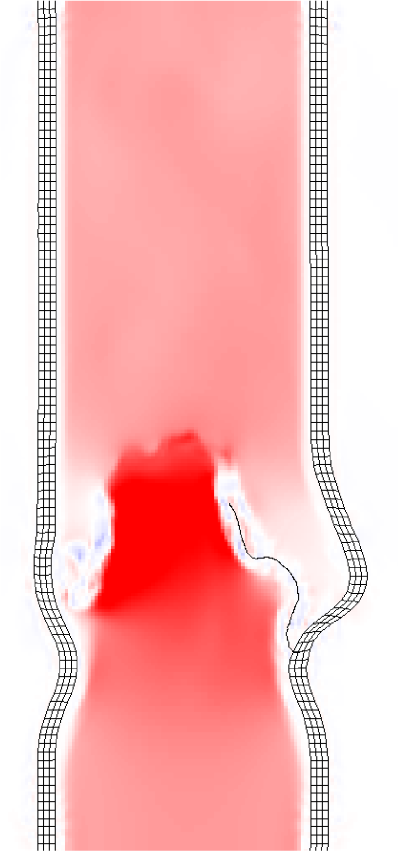
(d)

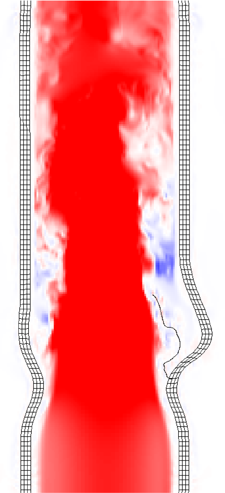
\psfragscanon\psfrag{s05}[t][t]{\color[rgb]{0,0,0}\begin{tabular}[]{c}Time (s)\end{tabular}}\psfrag{s06}[b][b]{\color[rgb]{0,0,0}\begin{tabular}[]{c}Flow Rate (ml/s)\end{tabular}}\psfrag{s08}[b][b]{\color[rgb]{0,0,0}\begin{tabular}[]{c}\end{tabular}}\psfrag{s10}{\color[rgb]{0,0,0}\begin{tabular}[]{c}\end{tabular}}\psfrag{s11}{\color[rgb]{0,0,0}\begin{tabular}[]{c}\end{tabular}}\psfrag{s12}[l][l]{\color[rgb]{0,0,0}N=256}\psfrag{s13}[l][l]{\color[rgb]{0,0,0}N=128}\psfrag{s14}[l][l]{\color[rgb]{0,0,0}N=256}\psfrag{x01}[t][t]{1}\psfrag{x02}[t][t]{1.5}\psfrag{x03}[t][t]{2}\psfrag{x04}[t][t]{2.5}\psfrag{x05}[t][t]{3}\psfrag{x06}[t][t]{3.5}\psfrag{x07}[t][t]{4}\psfrag{v01}[r][r]{-200}\psfrag{v02}[r][r]{-100}\psfrag{v03}[r][r]{0}\psfrag{v04}[r][r]{100}\psfrag{v05}[r][r]{200}\psfrag{v06}[r][r]{300}\psfrag{v07}[r][r]{400}\psfrag{v08}[r][r]{500}\psfrag{v09}[r][r]{600}\psfrag{v10}[r][r]{700}\includegraphics{flow_open.eps}

(e)

Figure 7: Valve leaflet configurations during valve opening shown at equally spaced times during the fourth simulated cardiac cycle for (7(a)) the coarser Cartesian grid (effective grid resolution of $N=128$) and (7(b)) the finer Cartesian grid (effective grid resolution of $N=256$). Panels (7(c)) and (7(d)) show the corresponding axial velocity profiles. Panel (7(e)) shows the computed flow rates, with the dashed lines indicating the time instants shown in panels (7(a))–(7(d)).

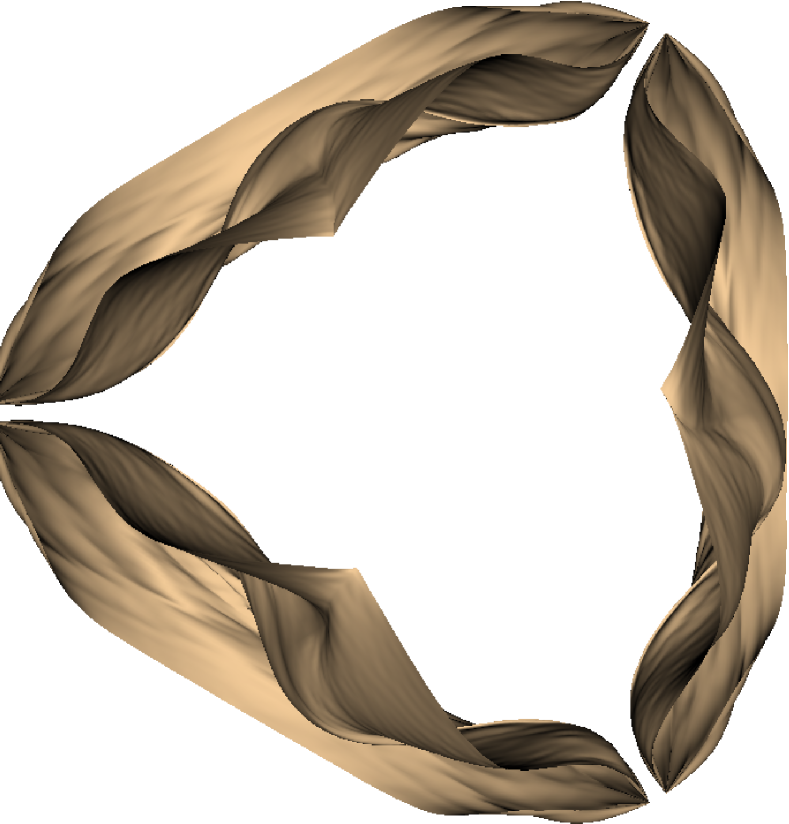
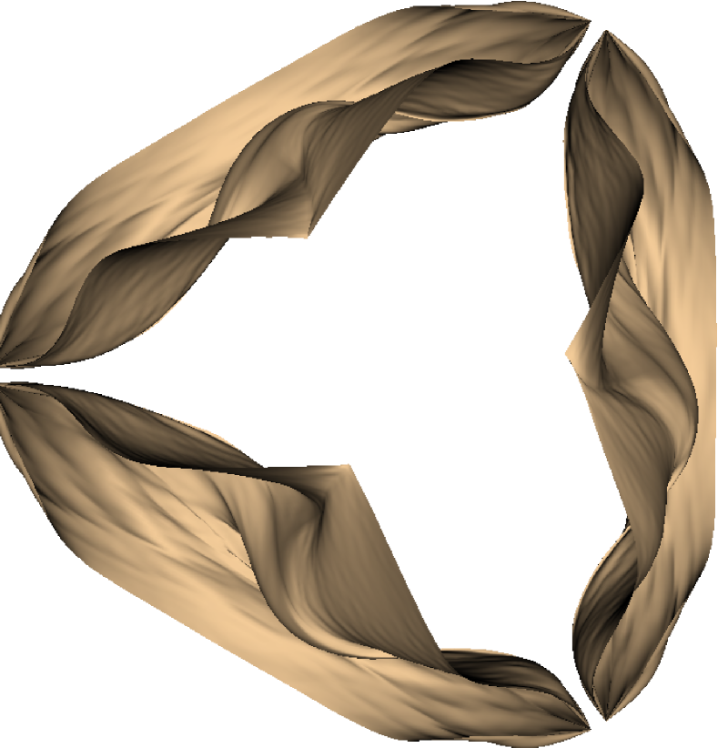
(a)

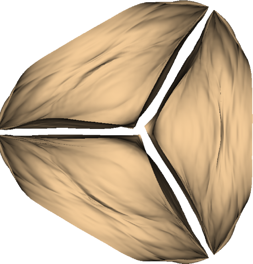
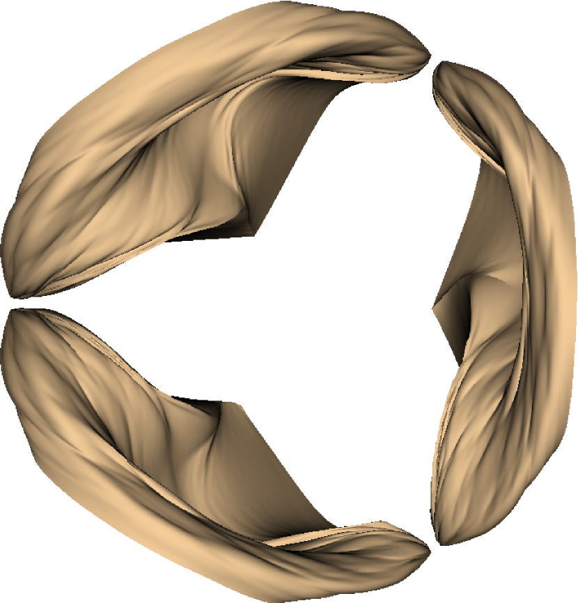
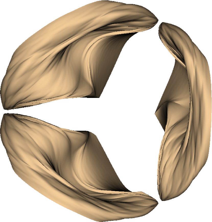
(b)

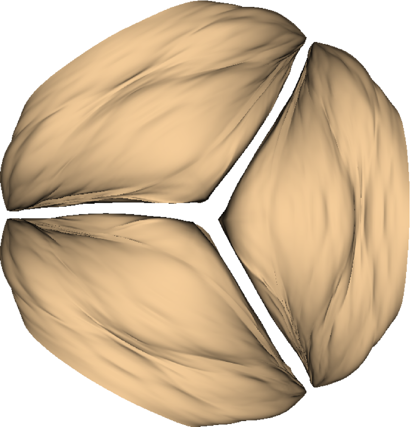
(c)

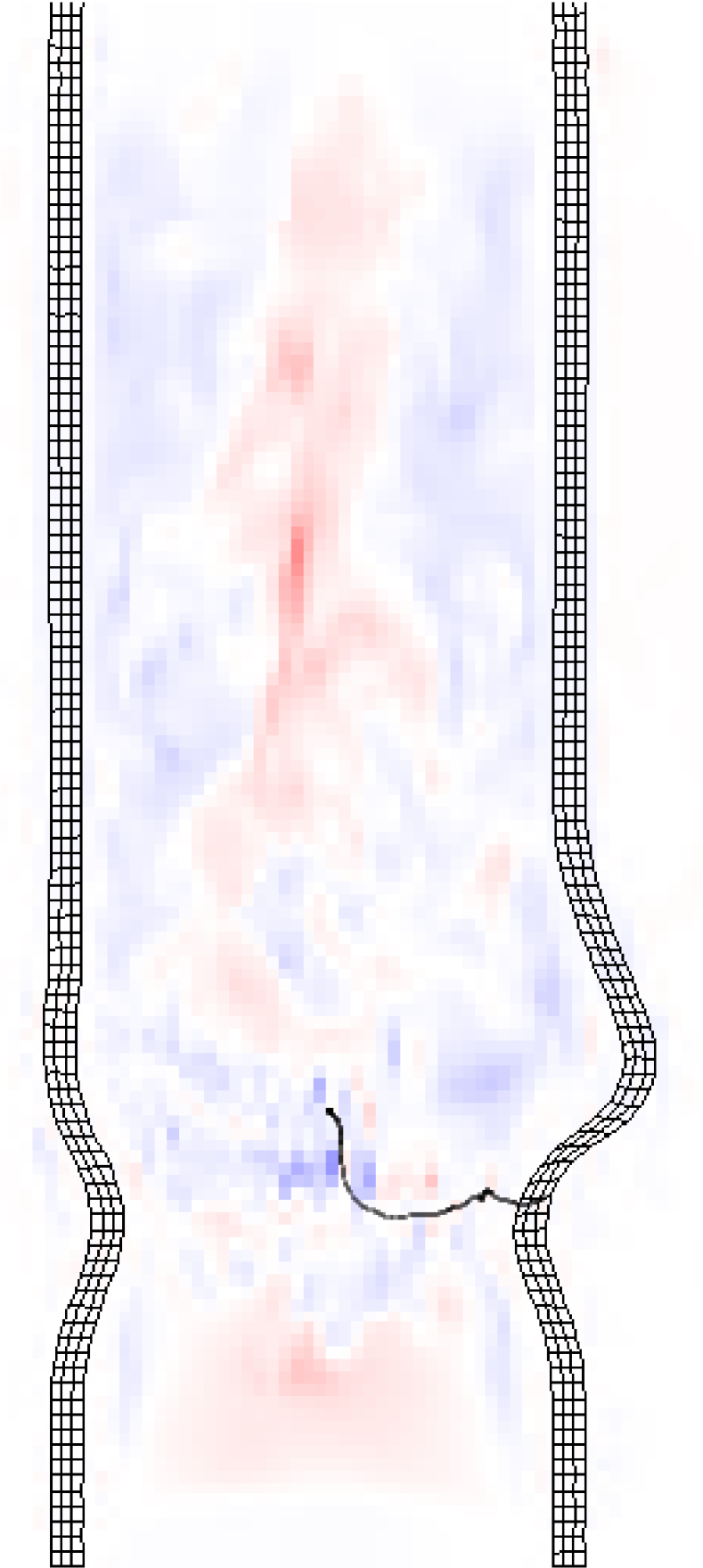
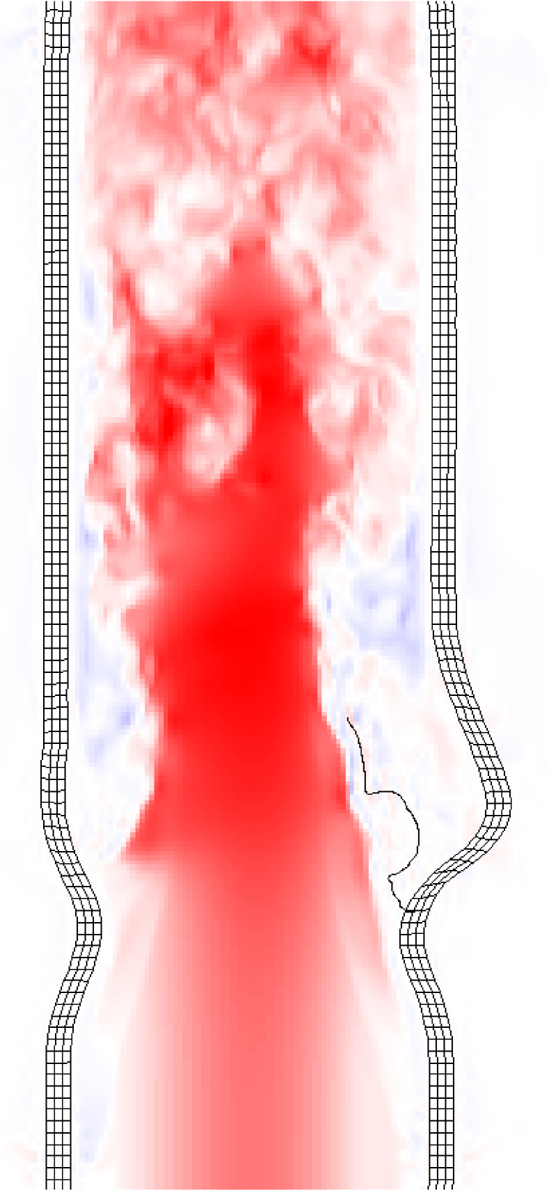
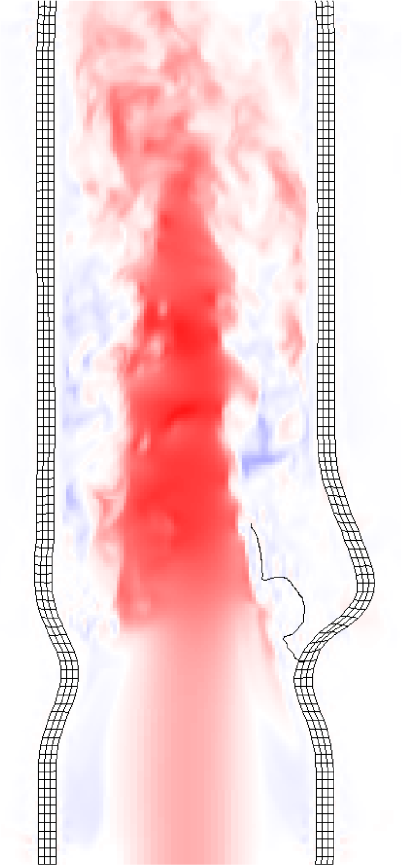
(d)

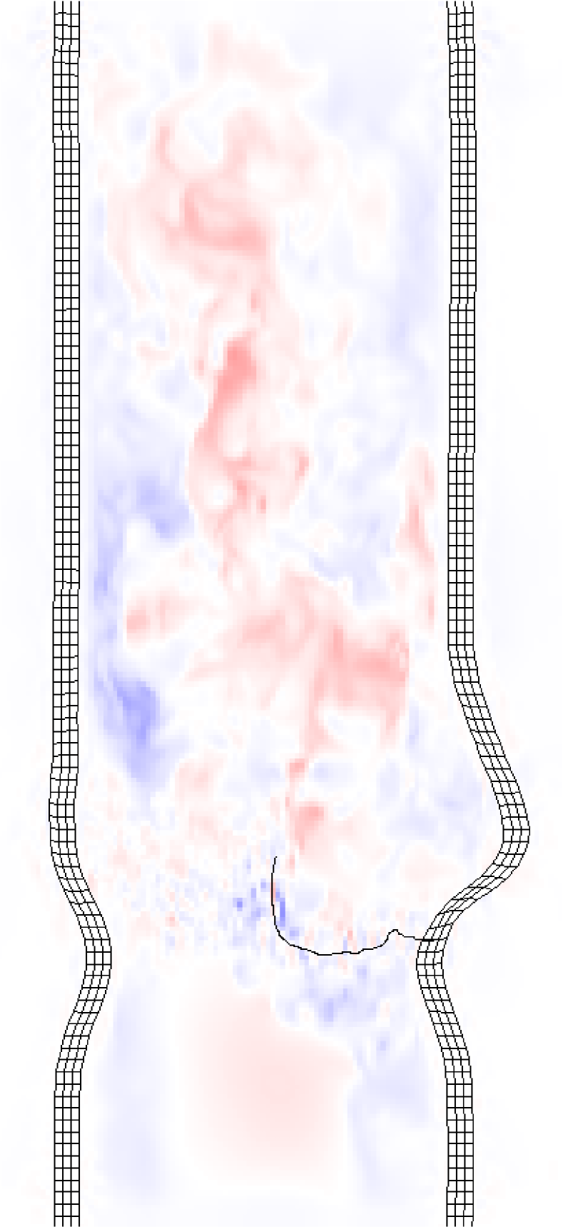
\psfragscanon\psfrag{s05}[t][t]{\color[rgb]{0,0,0}\begin{tabular}[]{c}Time (s)\end{tabular}}\psfrag{s06}[b][b]{\color[rgb]{0,0,0}\begin{tabular}[]{c}Flow Rate (ml/s)\end{tabular}}\psfrag{s08}[b][b]{\color[rgb]{0,0,0}\begin{tabular}[]{c}\end{tabular}}\psfrag{s10}{\color[rgb]{0,0,0}\begin{tabular}[]{c}\end{tabular}}\psfrag{s11}{\color[rgb]{0,0,0}\begin{tabular}[]{c}\end{tabular}}\psfrag{s12}[l][l]{\color[rgb]{0,0,0}N=256}\psfrag{s13}[l][l]{\color[rgb]{0,0,0}N=128}\psfrag{s14}[l][l]{\color[rgb]{0,0,0}N=256}\psfrag{x01}[t][t]{1}\psfrag{x02}[t][t]{1.5}\psfrag{x03}[t][t]{2}\psfrag{x04}[t][t]{2.5}\psfrag{x05}[t][t]{3}\psfrag{x06}[t][t]{3.5}\psfrag{x07}[t][t]{4}\psfrag{v01}[r][r]{-200}\psfrag{v02}[r][r]{-100}\psfrag{v03}[r][r]{0}\psfrag{v04}[r][r]{100}\psfrag{v05}[r][r]{200}\psfrag{v06}[r][r]{300}\psfrag{v07}[r][r]{400}\psfrag{v08}[r][r]{500}\psfrag{v09}[r][r]{600}\psfrag{v10}[r][r]{700}\includegraphics{flow_close.eps}

(e)

Figure 8: Similar to fig. 7, but here showing the dynamics of the closure of the aortic valve during the fourth cycle. In this case, the solid lines indicate the instants shown in the figure panels.

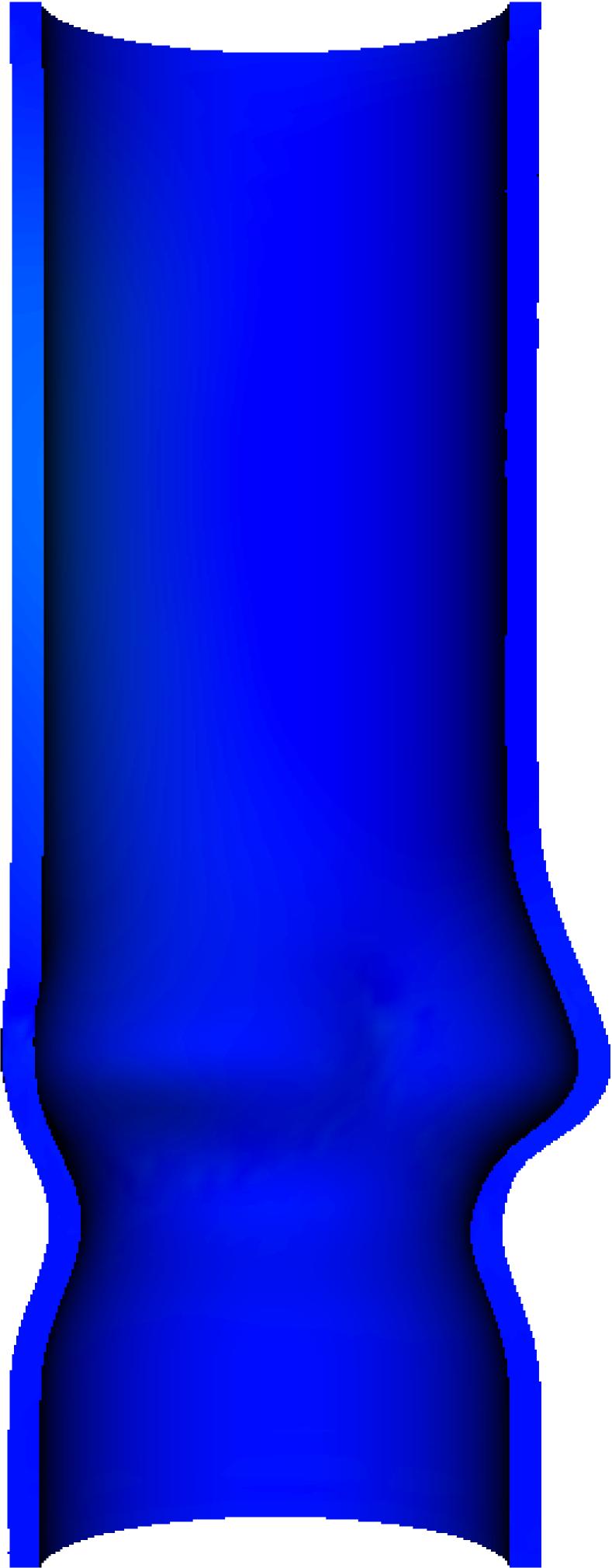
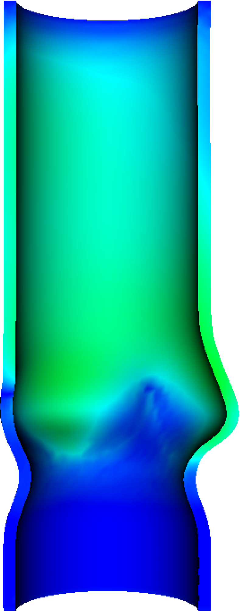
(a)

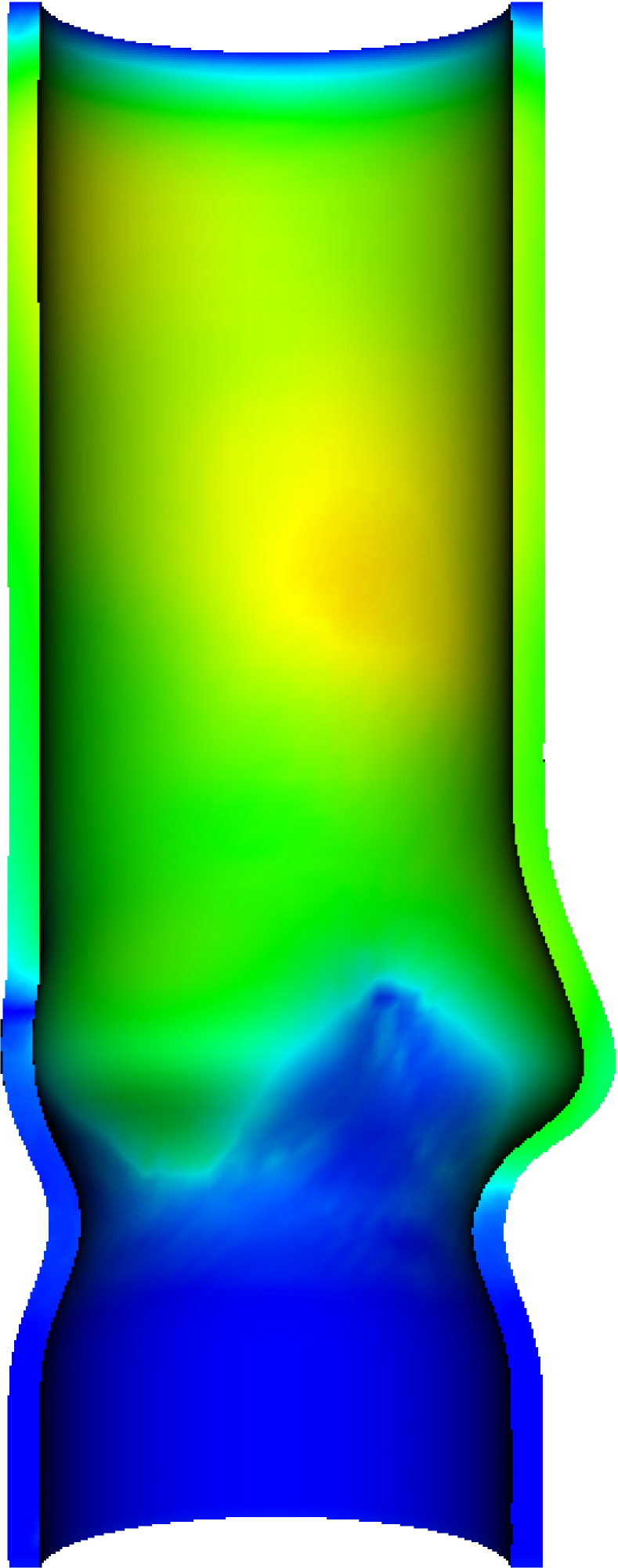
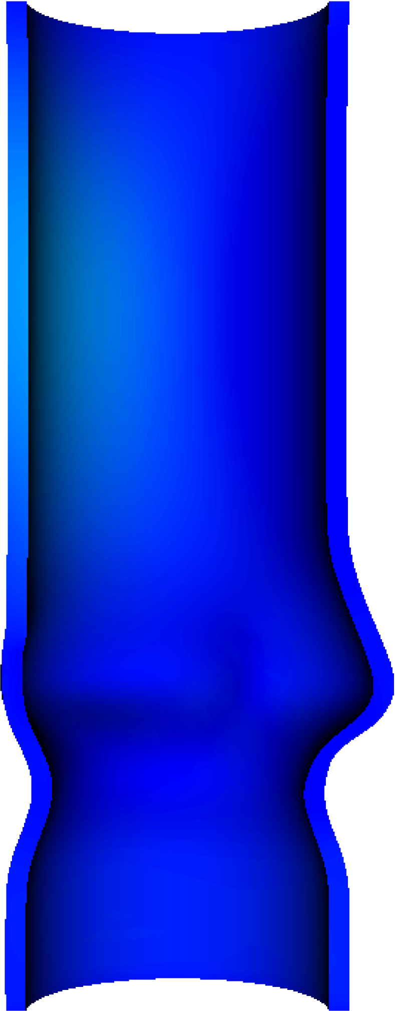
(b)

(c)

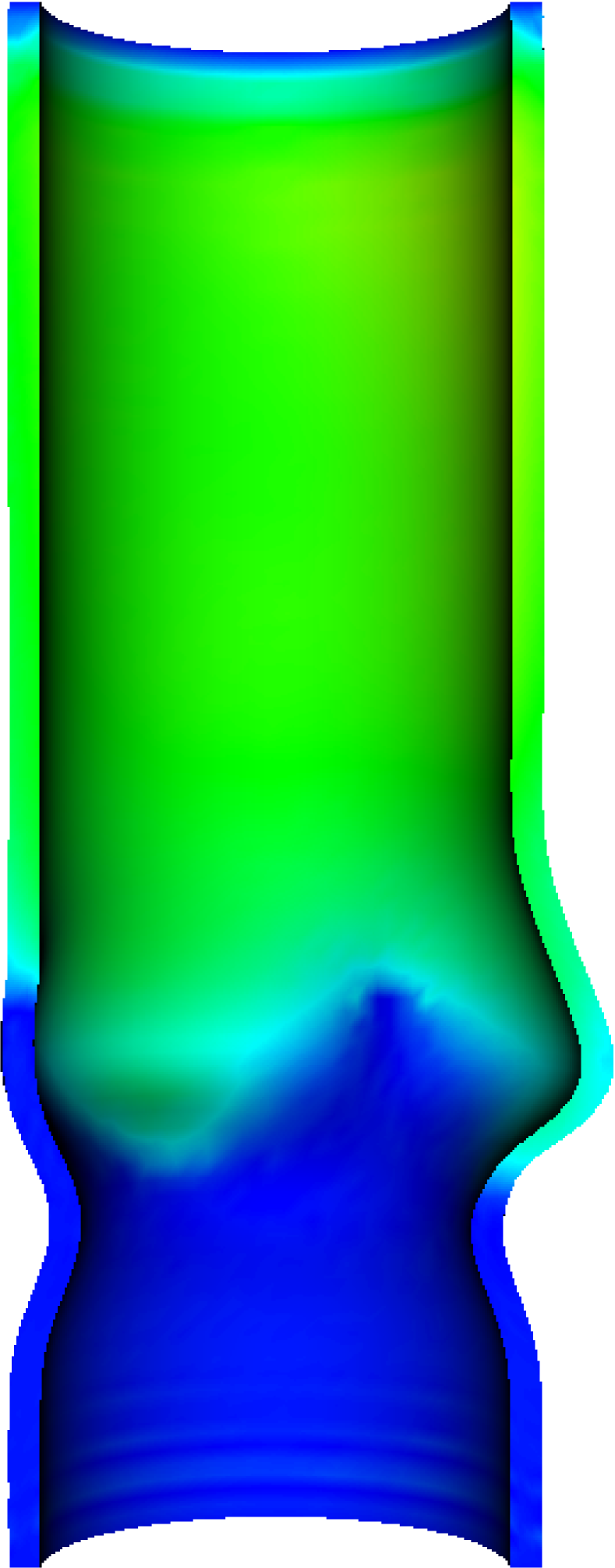
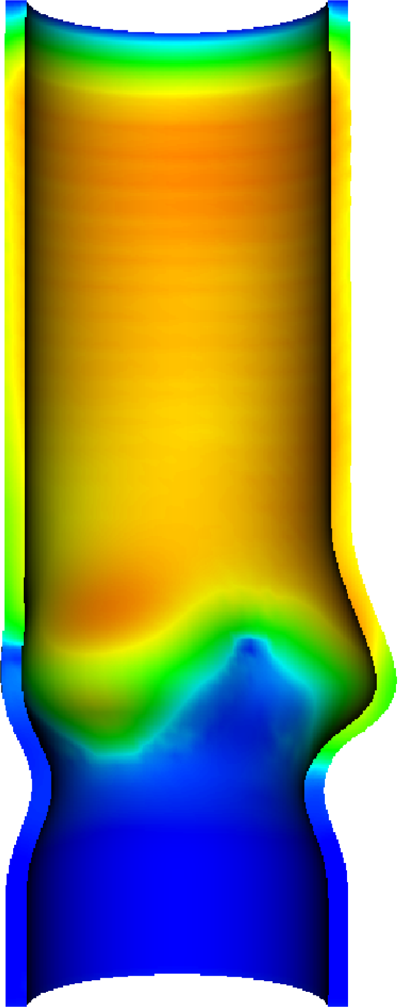
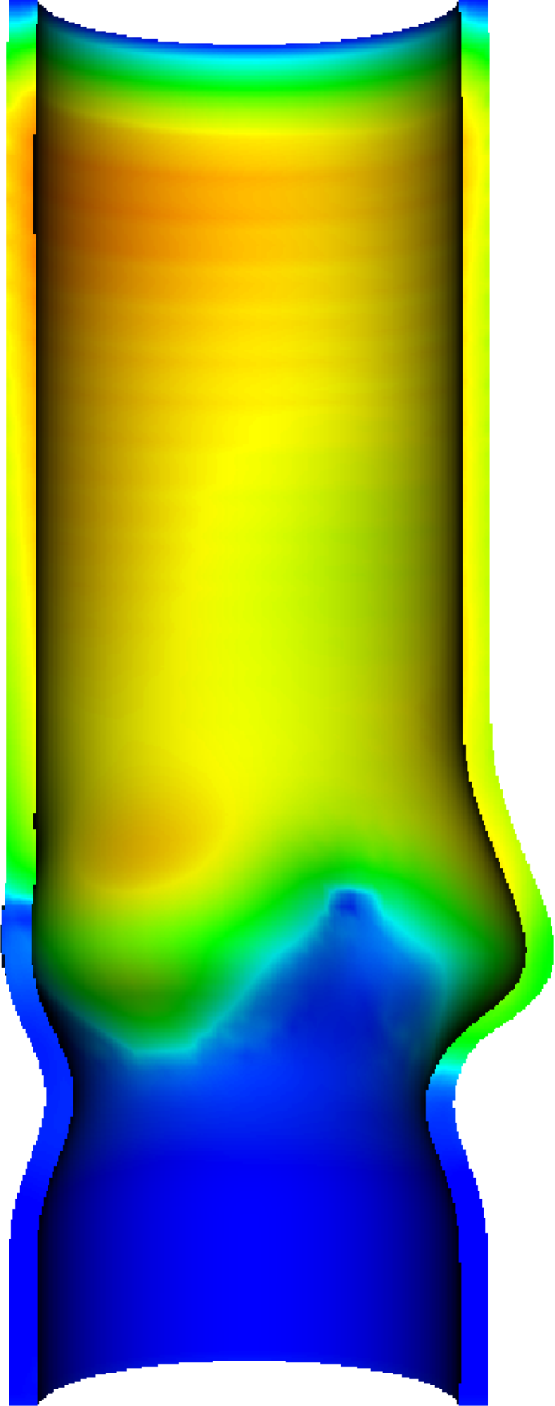
(d)

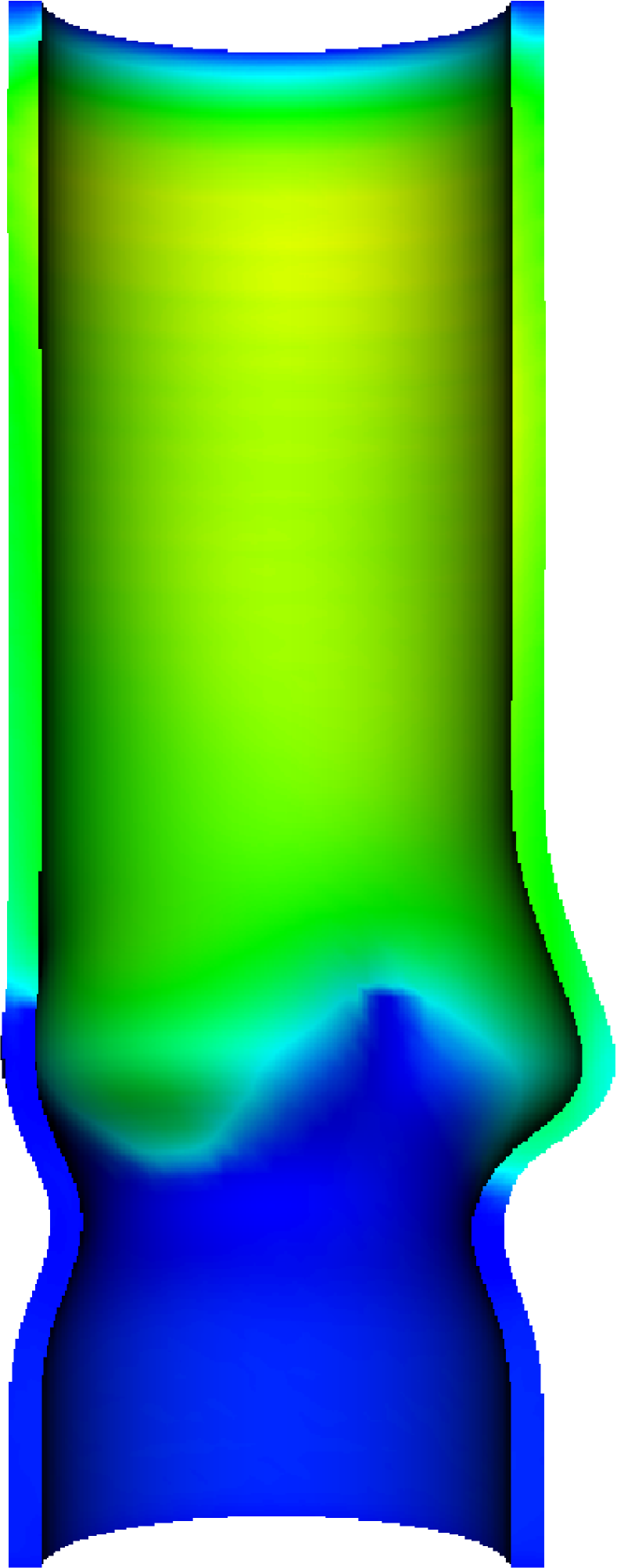
Figure 9: Displacement contours along the aortic root model. Panel (9(a)) shows displacement contours along the axial section of the aortic wall during valve opening, shown as the same time instants as in fig. 7, for the coarser Cartesian grid spacing. Panel (9(b)) is similar, but here shows results for the finer Cartesian grid spacing. Panels (9(c)) and (9(d)) are similar, but here show the displacement patterns during valve closure.

\psfragscanon\psfrag{s05}[t][t]{\color[rgb]{0,0,0}\begin{tabular}[]{c}Time(s)\end{tabular}}\psfrag{s06}[b][b]{\color[rgb]{0,0,0}\begin{tabular}[]{c}Displacement (mm)\end{tabular}}\psfrag{s10}{\color[rgb]{0,0,0}\begin{tabular}[]{c}\end{tabular}}\psfrag{s11}{\color[rgb]{0,0,0}\begin{tabular}[]{c}\end{tabular}}\psfrag{s12}[l][l]{\color[rgb]{0,0,0}N=256}\psfrag{s13}[l][l]{\color[rgb]{0,0,0}N=128}\psfrag{s14}[l][l]{\color[rgb]{0,0,0}N=256}\psfrag{x01}[t][t]{1}\psfrag{x02}[t][t]{1.5}\psfrag{x03}[t][t]{2}\psfrag{x04}[t][t]{2.5}\psfrag{x05}[t][t]{3}\psfrag{x06}[t][t]{3.5}\psfrag{x07}[t][t]{4}\psfrag{v01}[r][r]{-0.1}\psfrag{v02}[r][r]{0}\psfrag{v03}[r][r]{0.1}\psfrag{v04}[r][r]{0.2}\psfrag{v05}[r][r]{0.3}\psfrag{v06}[r][r]{0.4}\psfrag{v07}[r][r]{0.5}\psfrag{v08}[r][r]{0.6}\includegraphics{aorta_sym_dx_2.eps}

(a)

\psfragscanon\psfrag{s05}[t][t]{\color[rgb]{0,0,0}\begin{tabular}[]{c}Time(s)\end{tabular}}\psfrag{s06}[b][b]{\color[rgb]{0,0,0}\begin{tabular}[]{c}Displacement (mm)\end{tabular}}\psfrag{s10}{\color[rgb]{0,0,0}\begin{tabular}[]{c}\end{tabular}}\psfrag{s11}{\color[rgb]{0,0,0}\begin{tabular}[]{c}\end{tabular}}\psfrag{s12}[l][l]{\color[rgb]{0,0,0}N=256}\psfrag{s13}[l][l]{\color[rgb]{0,0,0}N=128}\psfrag{s14}[l][l]{\color[rgb]{0,0,0}N=256}\psfrag{x01}[t][t]{1}\psfrag{x02}[t][t]{1.5}\psfrag{x03}[t][t]{2}\psfrag{x04}[t][t]{2.5}\psfrag{x05}[t][t]{3}\psfrag{x06}[t][t]{3.5}\psfrag{x07}[t][t]{4}\psfrag{v01}[r][r]{-0.1}\psfrag{v02}[r][r]{0}\psfrag{v03}[r][r]{0.1}\psfrag{v04}[r][r]{0.2}\psfrag{v05}[r][r]{0.3}\psfrag{v06}[r][r]{0.4}\psfrag{v07}[r][r]{0.5}\psfrag{v08}[r][r]{0.6}\includegraphics{commis_sym_dx_2.eps}

(b)

\psfragscanon\psfrag{s05}[t][t]{\color[rgb]{0,0,0}\begin{tabular}[]{c}Time(s)\end{tabular}}\psfrag{s06}[b][b]{\color[rgb]{0,0,0}\begin{tabular}[]{c}Displacement (mm)\end{tabular}}\psfrag{s10}{\color[rgb]{0,0,0}\begin{tabular}[]{c}\end{tabular}}\psfrag{s11}{\color[rgb]{0,0,0}\begin{tabular}[]{c}\end{tabular}}\psfrag{s12}[l][l]{\color[rgb]{0,0,0}N=256}\psfrag{s13}[l][l]{\color[rgb]{0,0,0}N=128}\psfrag{s14}[l][l]{\color[rgb]{0,0,0}N=256}\psfrag{x01}[t][t]{1}\psfrag{x02}[t][t]{1.5}\psfrag{x03}[t][t]{2}\psfrag{x04}[t][t]{2.5}\psfrag{x05}[t][t]{3}\psfrag{x06}[t][t]{3.5}\psfrag{x07}[t][t]{4}\psfrag{v01}[r][r]{-0.1}\psfrag{v02}[r][r]{0}\psfrag{v03}[r][r]{0.1}\psfrag{v04}[r][r]{0.2}\psfrag{v05}[r][r]{0.3}\psfrag{v06}[r][r]{0.4}\psfrag{v07}[r][r]{0.5}\psfrag{v08}[r][r]{0.6}\includegraphics{STJ_sym_dx_2.eps}

(c)

\psfragscanon\psfrag{s05}[t][t]{\color[rgb]{0,0,0}\begin{tabular}[]{c}Time(s)\end{tabular}}\psfrag{s06}[b][b]{\color[rgb]{0,0,0}\begin{tabular}[]{c}Displacement (mm)\end{tabular}}\psfrag{s10}{\color[rgb]{0,0,0}\begin{tabular}[]{c}\end{tabular}}\psfrag{s11}{\color[rgb]{0,0,0}\begin{tabular}[]{c}\end{tabular}}\psfrag{s12}[l][l]{\color[rgb]{0,0,0}N=256}\psfrag{s13}[l][l]{\color[rgb]{0,0,0}N=128}\psfrag{s14}[l][l]{\color[rgb]{0,0,0}N=256}\psfrag{x01}[t][t]{1}\psfrag{x02}[t][t]{1.5}\psfrag{x03}[t][t]{2}\psfrag{x04}[t][t]{2.5}\psfrag{x05}[t][t]{3}\psfrag{x06}[t][t]{3.5}\psfrag{x07}[t][t]{4}\psfrag{v01}[r][r]{-0.05}\psfrag{v02}[r][r]{0}\psfrag{v03}[r][r]{0.05}\psfrag{v04}[r][r]{0.1}\psfrag{v05}[r][r]{0.15}\psfrag{v06}[r][r]{0.2}\psfrag{v07}[r][r]{0.25}\psfrag{v08}[r][r]{0.3}\psfrag{v09}[r][r]{0.35}\psfrag{v10}[r][r]{0.4}\psfrag{v11}[r][r]{0.45}\includegraphics{sinus_sym_dx.eps}

(d)

Figure 10: Displacements of the deformable aortic root model at four locations: (10(a)) the straight portion of the aorta; (10(b)) just above one of the commissures; (10(c)) the sinotubular junction; and (10(d)) the middle of the sinus.

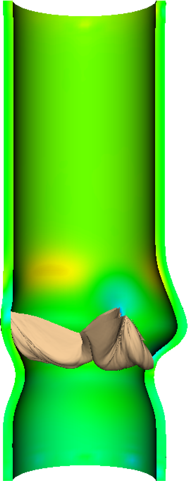
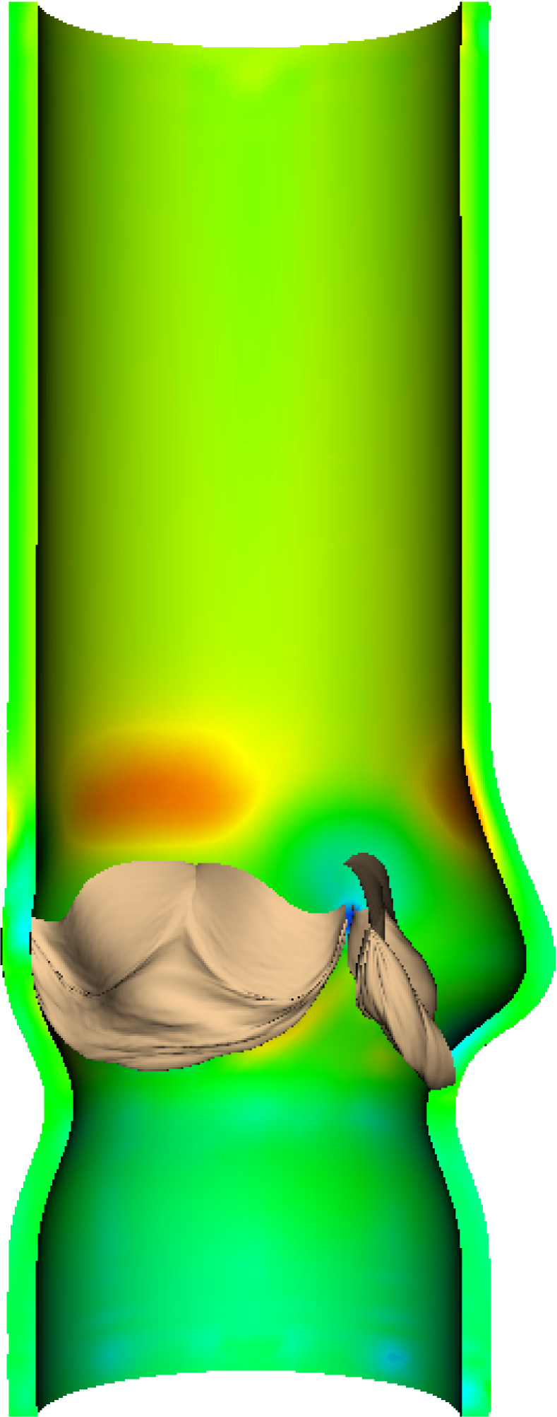
(a)

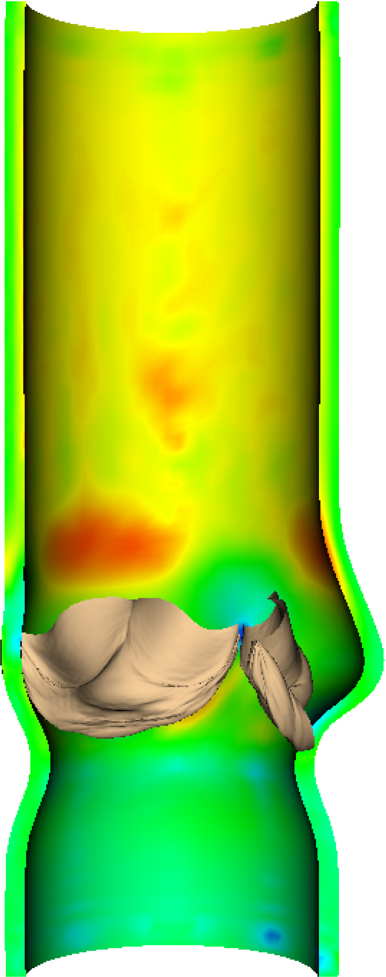
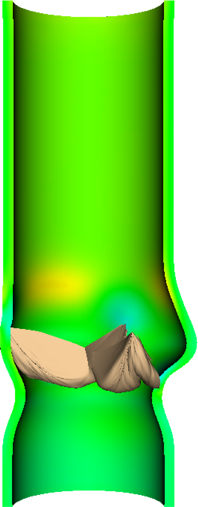
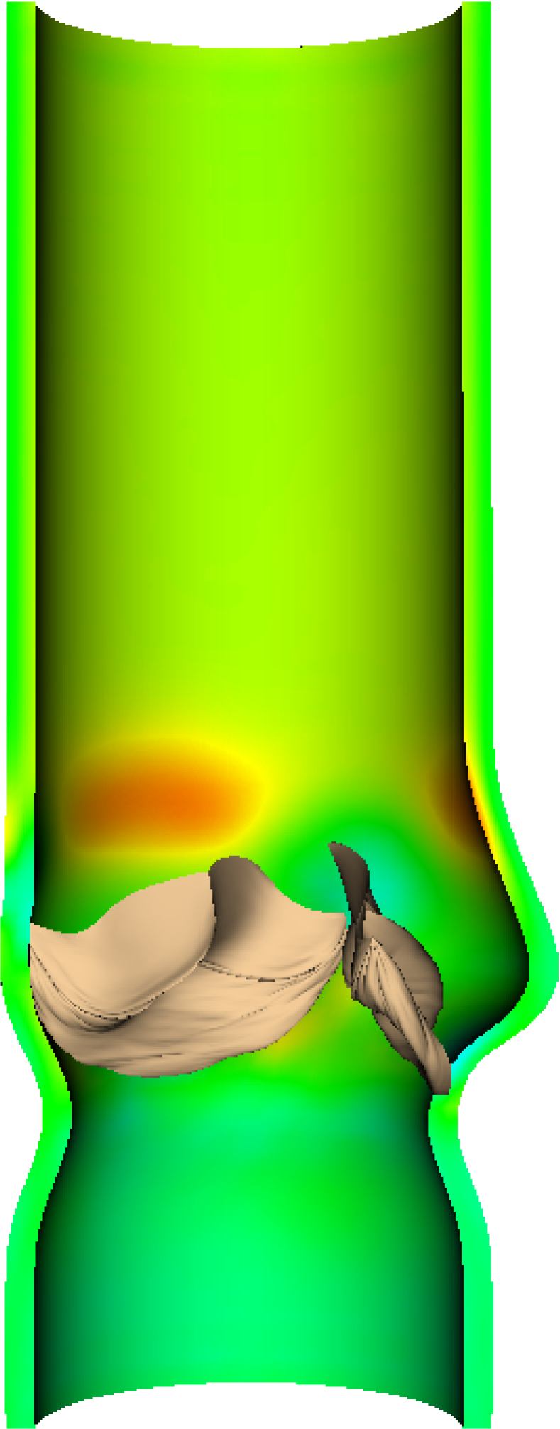
(b)

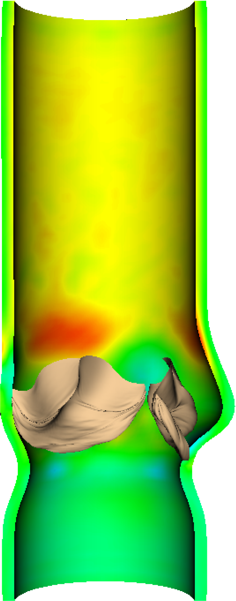
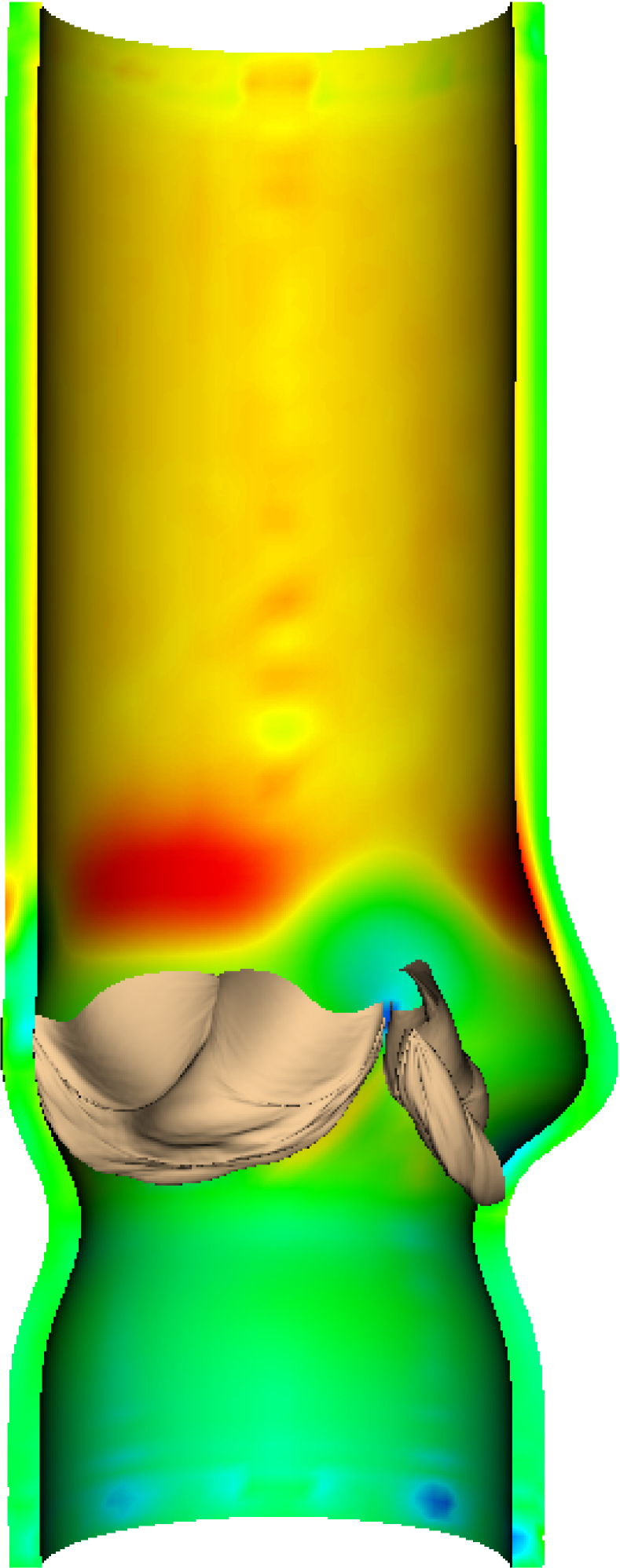
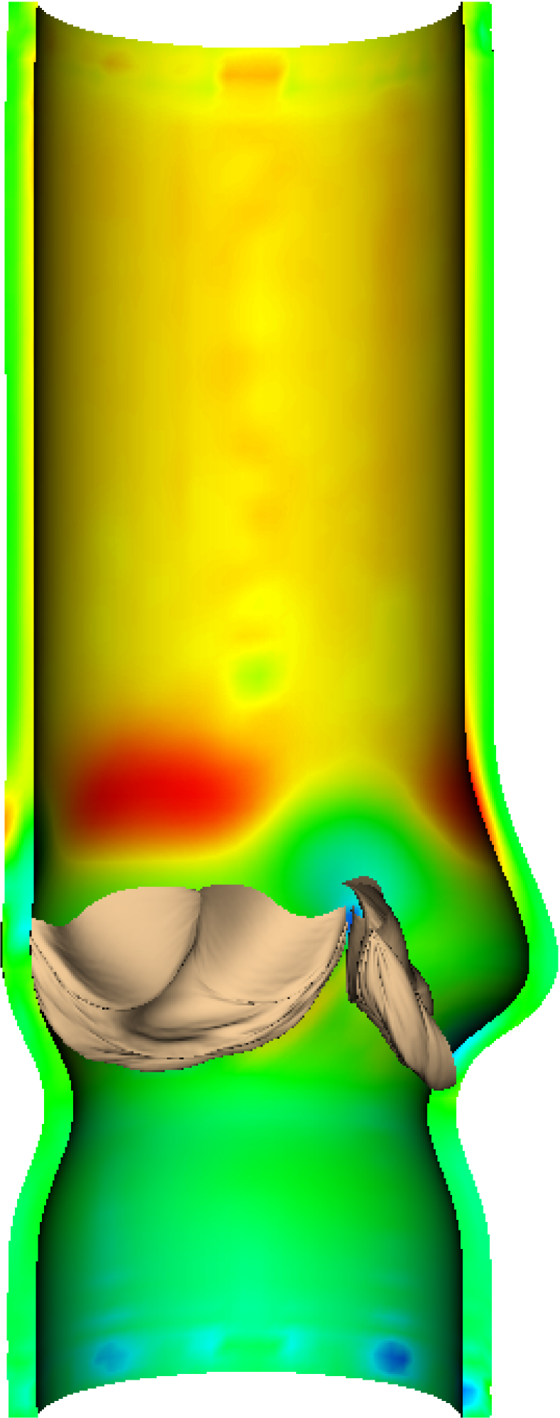
(c)

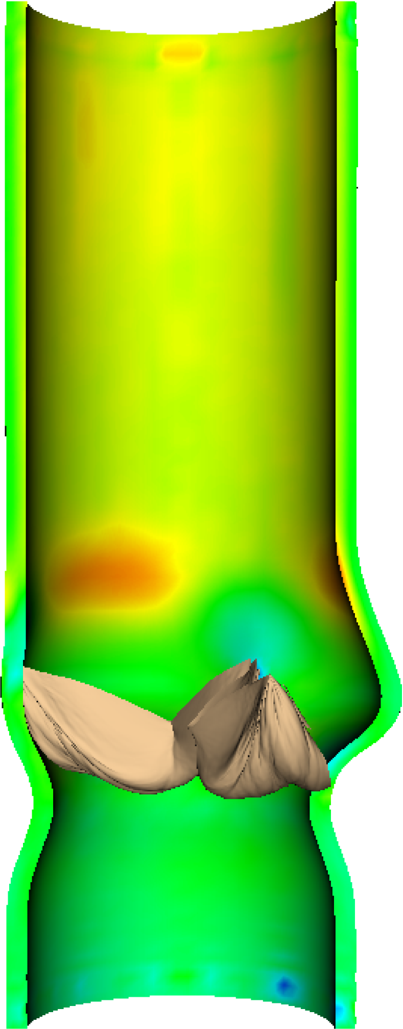
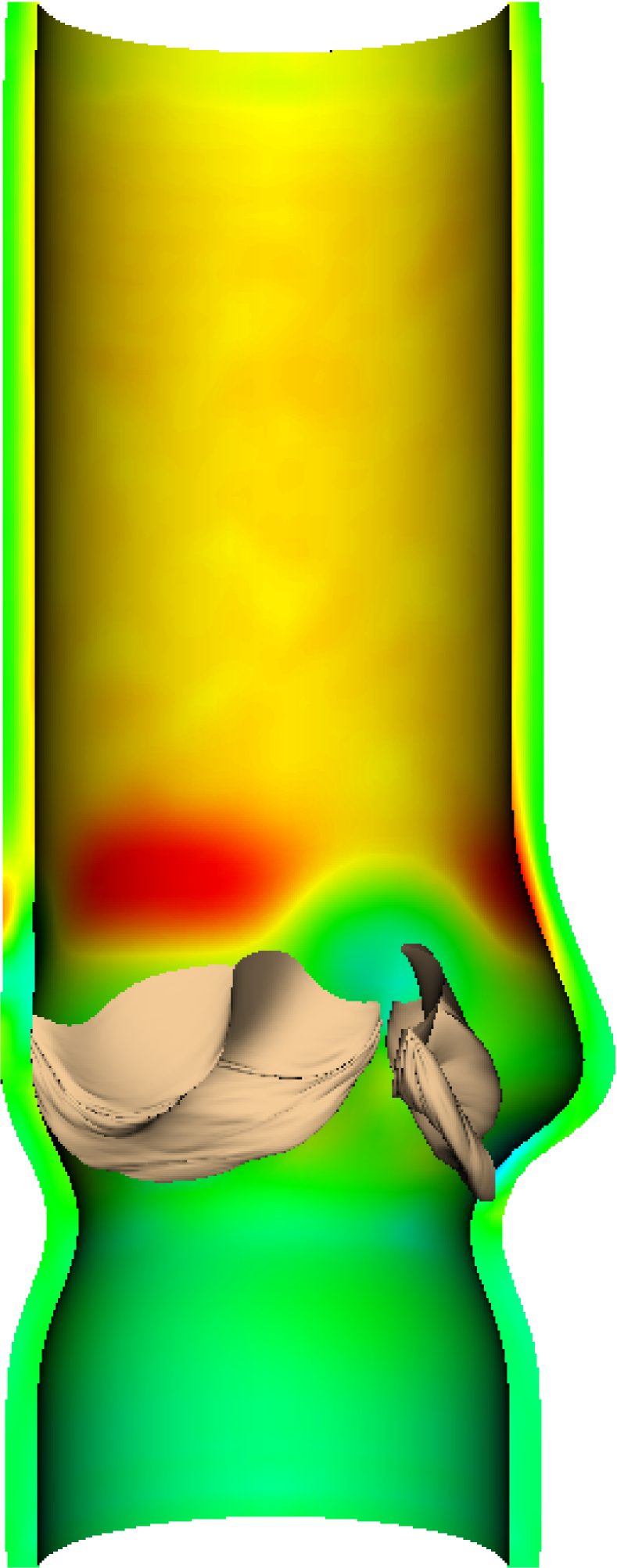
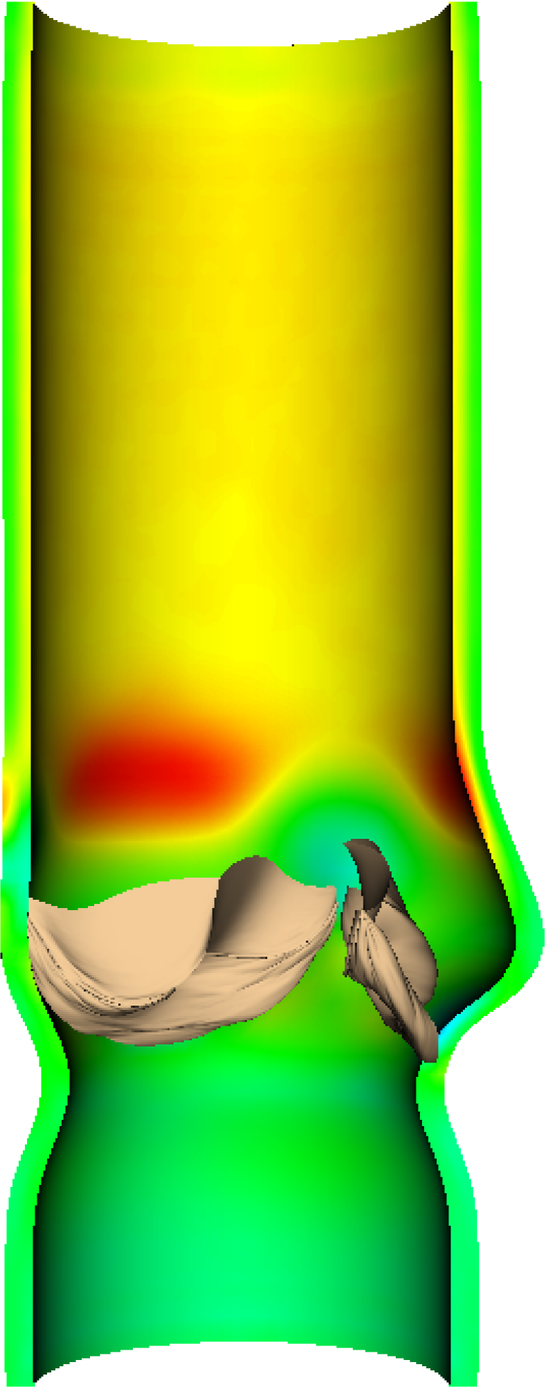
(d)

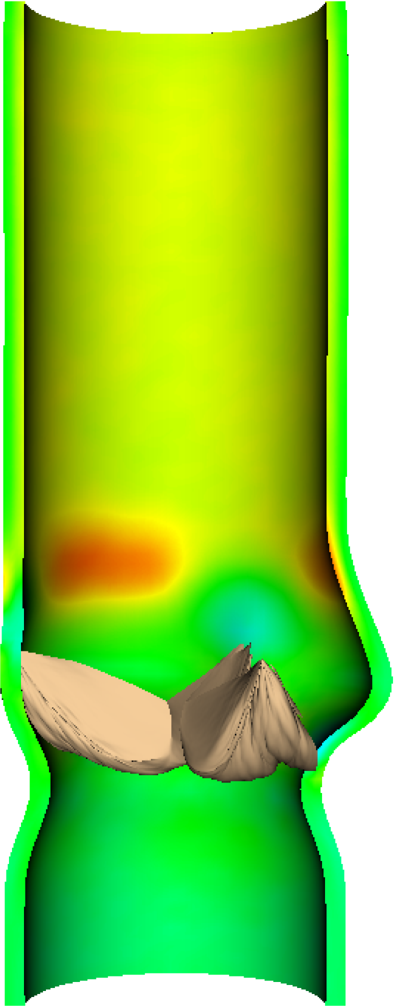
Figure 11: Maximum principal stress contours along the aortic root model. Panel (11(a)) shows displacement contours along the axial section of the aortic wall during valve opening, shown as the same time instants as in fig. 7, for the coarser Cartesian grid spacing. Panel (11(b)) is similar, but here shows results for the finer Cartesian grid spacing. Panels (11(c)) and (11(d)) are similar, but here show the displacement patterns durning valve closure.

\psfragscanon\psfrag{s05}[t][t]{\color[rgb]{0,0,0}\begin{tabular}[]{c}Time(s)\end{tabular}}\psfrag{s06}[b][b]{\color[rgb]{0,0,0}\begin{tabular}[]{c}First Principal Stress (kPa)\end{tabular}}\psfrag{s10}{\color[rgb]{0,0,0}\begin{tabular}[]{c}\end{tabular}}\psfrag{s11}{\color[rgb]{0,0,0}\begin{tabular}[]{c}\end{tabular}}\psfrag{s12}[l][l]{\color[rgb]{0,0,0}N=256}\psfrag{s13}[l][l]{\color[rgb]{0,0,0}N=128}\psfrag{s14}[l][l]{\color[rgb]{0,0,0}N=256}\psfrag{x01}[t][t]{1}\psfrag{x02}[t][t]{1.5}\psfrag{x03}[t][t]{2}\psfrag{x04}[t][t]{2.5}\psfrag{x05}[t][t]{3}\psfrag{x06}[t][t]{3.5}\psfrag{x07}[t][t]{4}\psfrag{v01}[r][r]{60}\psfrag{v02}[r][r]{70}\psfrag{v03}[r][r]{80}\psfrag{v04}[r][r]{90}\psfrag{v05}[r][r]{100}\psfrag{v06}[r][r]{110}\psfrag{v07}[r][r]{120}\psfrag{v08}[r][r]{130}\psfrag{v09}[r][r]{140}\psfrag{v10}[r][r]{150}\includegraphics{aorta_sym_sp1.eps}

(a)

\psfragscanon\psfrag{s05}[t][t]{\color[rgb]{0,0,0}\begin{tabular}[]{c}Time(s)\end{tabular}}\psfrag{s06}[b][b]{\color[rgb]{0,0,0}\begin{tabular}[]{c}First Principal Stress (kPa)\end{tabular}}\psfrag{s10}{\color[rgb]{0,0,0}\begin{tabular}[]{c}\end{tabular}}\psfrag{s11}{\color[rgb]{0,0,0}\begin{tabular}[]{c}\end{tabular}}\psfrag{s12}[l][l]{\color[rgb]{0,0,0}N=256}\psfrag{s13}[l][l]{\color[rgb]{0,0,0}N=128}\psfrag{s14}[l][l]{\color[rgb]{0,0,0}N=256}\psfrag{x01}[t][t]{1}\psfrag{x02}[t][t]{1.5}\psfrag{x03}[t][t]{2}\psfrag{x04}[t][t]{2.5}\psfrag{x05}[t][t]{3}\psfrag{x06}[t][t]{3.5}\psfrag{x07}[t][t]{4}\psfrag{v01}[r][r]{60}\psfrag{v02}[r][r]{80}\psfrag{v03}[r][r]{100}\psfrag{v04}[r][r]{120}\psfrag{v05}[r][r]{140}\psfrag{v06}[r][r]{160}\psfrag{v07}[r][r]{180}\includegraphics{commiss_sym_sp1.eps}

(b)

\psfragscanon\psfrag{s05}[t][t]{\color[rgb]{0,0,0}\begin{tabular}[]{c}Time(s)\end{tabular}}\psfrag{s06}[b][b]{\color[rgb]{0,0,0}\begin{tabular}[]{c}First Principal Stress (kPa)\end{tabular}}\psfrag{s10}{\color[rgb]{0,0,0}\begin{tabular}[]{c}\end{tabular}}\psfrag{s11}{\color[rgb]{0,0,0}\begin{tabular}[]{c}\end{tabular}}\psfrag{s12}[l][l]{\color[rgb]{0,0,0}N=256}\psfrag{s13}[l][l]{\color[rgb]{0,0,0}N=128}\psfrag{s14}[l][l]{\color[rgb]{0,0,0}N=256}\psfrag{x01}[t][t]{1}\psfrag{x02}[t][t]{1.5}\psfrag{x03}[t][t]{2}\psfrag{x04}[t][t]{2.5}\psfrag{x05}[t][t]{3}\psfrag{x06}[t][t]{3.5}\psfrag{x07}[t][t]{4}\psfrag{v01}[r][r]{90}\psfrag{v02}[r][r]{100}\psfrag{v03}[r][r]{110}\psfrag{v04}[r][r]{120}\psfrag{v05}[r][r]{130}\psfrag{v06}[r][r]{140}\psfrag{v07}[r][r]{150}\psfrag{v08}[r][r]{160}\psfrag{v09}[r][r]{170}\psfrag{v10}[r][r]{180}\psfrag{v11}[r][r]{190}\includegraphics{STJ_sym_sp1.eps}

(c)

\psfragscanon\psfrag{s05}[t][t]{\color[rgb]{0,0,0}\begin{tabular}[]{c}Time(s)\end{tabular}}\psfrag{s06}[b][b]{\color[rgb]{0,0,0}\begin{tabular}[]{c}First Principal Stress (kPa)\end{tabular}}\psfrag{s10}{\color[rgb]{0,0,0}\begin{tabular}[]{c}\end{tabular}}\psfrag{s11}{\color[rgb]{0,0,0}\begin{tabular}[]{c}\end{tabular}}\psfrag{s12}[l][l]{\color[rgb]{0,0,0}N=256}\psfrag{s13}[l][l]{\color[rgb]{0,0,0}N=128}\psfrag{s14}[l][l]{\color[rgb]{0,0,0}N=256}\psfrag{x01}[t][t]{1}\psfrag{x02}[t][t]{1.5}\psfrag{x03}[t][t]{2}\psfrag{x04}[t][t]{2.5}\psfrag{x05}[t][t]{3}\psfrag{x06}[t][t]{3.5}\psfrag{x07}[t][t]{4}\psfrag{v01}[r][r]{18}\psfrag{v02}[r][r]{20}\psfrag{v03}[r][r]{22}\psfrag{v04}[r][r]{24}\psfrag{v05}[r][r]{26}\psfrag{v06}[r][r]{28}\psfrag{v07}[r][r]{30}\psfrag{v08}[r][r]{32}\psfrag{v09}[r][r]{34}\includegraphics{sinus_sym_sp1.eps}

(d)

Figure 12: Maximum principal stress of the deformable aortic root model at four locations: (12(a)) the straight portion of the aorta; (12(b)) just above one of the commissures; (12(c)) the sinotubular junction; and (12(d)) the middle of the sinus.

A dynamic fluid-structure interaction analysis is performed that includes four cardiac cycles, including an initialization cycle and three cycles in which the model has attained periodic steady state. (Data are reported only for the beats in which the model has reached steady state.) Fig. 6 shows the prescribed left-ventricular driving pressure along with the computed aortic loading pressure determined by the coupled Windkessel model and the computed flow rate through the symmetric aortic root. We emphasize that the flow rate is not imposed in the model, but rather is predicted by the fluid-structure interaction analysis. For the simulations using the coarser Cartesian spacing, $h=0.78125~{}\text{mm}$, stroke volume is 96.2 ml, peak flow rate is 591.5 ml/s, and cardiac output is 6.5 l/min. For the finer Cartesian grid spacing, $h=0.3906~{}\text{mm}$, stroke volume is 100.2 ml, peak flow rate is 643.8 ml/s, and cardiac output is 6.8 l/min. Both sets of simulation results are within 15% of the hemodynamic parameters of the subject-specific clinical data used to determine the driving pressure and the Windkessel model parameters stergiopulos1999 ; murgo1980 . Specifically, the driving pressure and the Windkessel model parameters used in this work were based on clinical measurements from a subject with stroke volume of 100 ml, peak flow rate of 560 ml/s, and cardiac output of 6.8 l/min, as reported by Murgo et al. murgo1980 . The simulations also capture the incisura in the flow profile corresponding to the backward flow generated by the leaflets. The backward flow volume is 1.77 $\pm$ 0.11 ml, or 1.8% of the stroke volume, for the coarser grid spacing, and 1.52 $\pm$ 0.059 ml, or 1.5% of the stroke volume, for the finer grid spacing. The net forward flow volume (i.e., into the aorta) following leaflet coaptation is 0.02 $\pm$ 0.01 ml. This forward flow results from interactions between the elastic aortic root and the dynamic downstream loading pressure. As the downstream pressure falls during diastole, the load on the aortic wall and leaflets decreases and allows the aortic root to gradually push fluid into the distal aorta.

The model captures the opening and closing dynamics of the valve at both Cartesian grid spacings. Fig. 7 shows the leaflets being pushed apart along with the formation of the vortices that help the leaflets to close at the end of systole. Fig. 8 shows that although there is some net flow towards the left ventricle as the valve closes, once the valve closes, no further flow is allowed between the aorta and the left ventricle.

Fig. 9 shows the distribution of the structural displacements in the aortic root, and fig. 10 shows displacement as a function of time at four selected locations: the center of the sinus; the sinotubular junction; the commissure; and the ascending aorta. Notice that after the first cardiac cycle, the displacements are essentially periodic in time. Cartesian grid resolution has a minimal effect on the range of displacements except for the displacements measured at the commissure. The largest amplitude is observed in the ascending aorta ($0.58\pm 0.05$ mm) and at the sinotubular junction ($0.52\pm 0.02$ mm). A measure of aortic stiffness is the radial pulsation, i.e., the ratio of the difference between systolic radius and diastolic radius to the average radius nichols2011 , which in the present analysis was approximately 3.9% for the coarser Cartesian grid spacing and 2.9% for the finer Cartesian grid spacing. These values are similar to the value of 2.5% reported in refs. humphrey2002 and nichols2011 for the ascending aorta. The distribution of the displacements was also in good agreement with literature data, with the displacements in the aortic root greater in the sinotubular junction, and at the commissures than in the sinuses, as reported also by Lansac lansac2002 .

The distribution of the maximum principal stress in the aortic root follows a distribution similar to that of the displacement, with the maximum stresses concentrated in the sinotubular junction, just above the sinuses, as shown in fig. 11. Stress in the aortic root follows the pulsatile waveform of the pressure; see fig. 12. Both Cartesian grid spacings yield similar stress distributions; compare fig. 11 panels (11(a)) and (11(b)), but fig. 12 shows some differences along the sinotubular junction and within the sinuses. The maximum principal stress in the sinuses is 20% of that observed in the rest of the aortic root. The distribution, and the range of the maximum principal stress predicted by our model, is in agreement with other analyses available in literature, in particular with the 220 kPa peak of the maximum principal stress in the sinotubular junction reported by Conti et al. conti2010 .

3.3.2 Asymmetric model

\psfragscanon\psfrag{s05}[b][b]{\color[rgb]{0,0,0}\begin{tabular}[]{c}Pressure (mmHg)\end{tabular}}\psfrag{s06}[t][t]{\color[rgb]{0,0,0}\begin{tabular}[]{c}Time (s)\end{tabular}}\psfrag{s10}{\color[rgb]{0,0,0}\begin{tabular}[]{c}\end{tabular}}\psfrag{s11}{\color[rgb]{0,0,0}\begin{tabular}[]{c}\end{tabular}}\psfrag{s12}[l][l]{\color[rgb]{0,0,0}Left Ventricle}\psfrag{s13}[l][l]{\color[rgb]{0,0,0}Aorta}\psfrag{s14}[l][l]{\color[rgb]{0,0,0}Left Ventricle}\psfrag{x01}[t][t]{1}\psfrag{x02}[t][t]{1.5}\psfrag{x03}[t][t]{2}\psfrag{x04}[t][t]{2.5}\psfrag{x05}[t][t]{3}\psfrag{x06}[t][t]{3.5}\psfrag{x07}[t][t]{4}\psfrag{v01}[r][r]{0}\psfrag{v02}[r][r]{20}\psfrag{v03}[r][r]{40}\psfrag{v04}[r][r]{60}\psfrag{v05}[r][r]{80}\psfrag{v06}[r][r]{100}\psfrag{v07}[r][r]{120}\includegraphics{pres_asym.eps}

(a)

\psfragscanon\psfrag{s03}[t][t]{\color[rgb]{0,0,0}\begin{tabular}[]{c}Time (s)\end{tabular}}\psfrag{s04}[b][b]{\color[rgb]{0,0,0}\begin{tabular}[]{c}Flow Rate (ml/s)\end{tabular}}\psfrag{x01}[t][t]{1}\psfrag{x02}[t][t]{1.5}\psfrag{x03}[t][t]{2}\psfrag{x04}[t][t]{2.5}\psfrag{x05}[t][t]{3}\psfrag{x06}[t][t]{3.5}\psfrag{x07}[t][t]{4}\psfrag{v01}[r][r]{-200}\psfrag{v02}[r][r]{-100}\psfrag{v03}[r][r]{0}\psfrag{v04}[r][r]{100}\psfrag{v05}[r][r]{200}\psfrag{v06}[r][r]{300}\psfrag{v07}[r][r]{400}\psfrag{v08}[r][r]{500}\psfrag{v09}[r][r]{600}\includegraphics{flow_asym.eps}

(b)

Figure 13: Results of a dynamic fluid-structure interaction analysis of the asymmetric aortic root over the final three simulated cardiac cycles. (13(a)) Prescribed left-ventricular driving pressure and computed aortic loading pressure, and (13(b)) computed flow rate, in which the dashed vertical lines highlight the moment that the valve leaflets open and the solid vertical lines highlight the moment that the valve leaflets close. Large oscillations indicate the reverberations of the aortic valve leaflets upon closure.

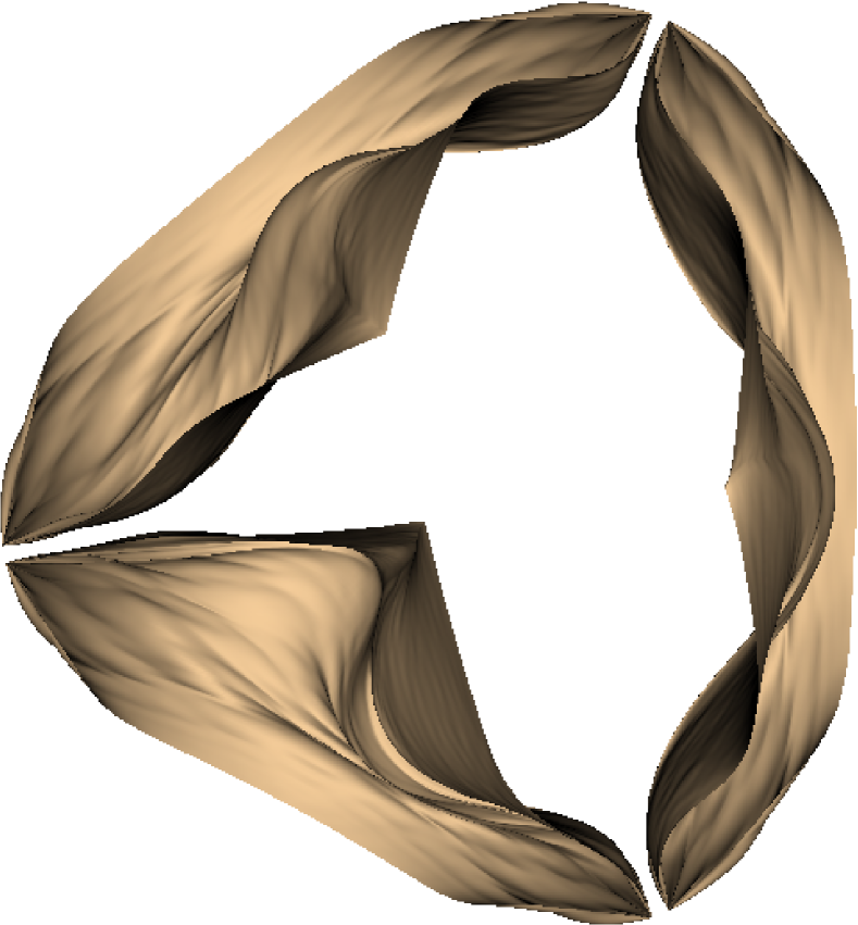
(a)

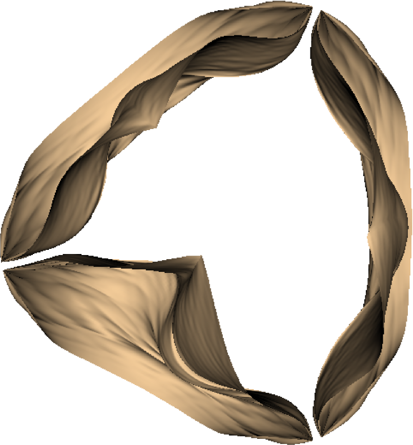
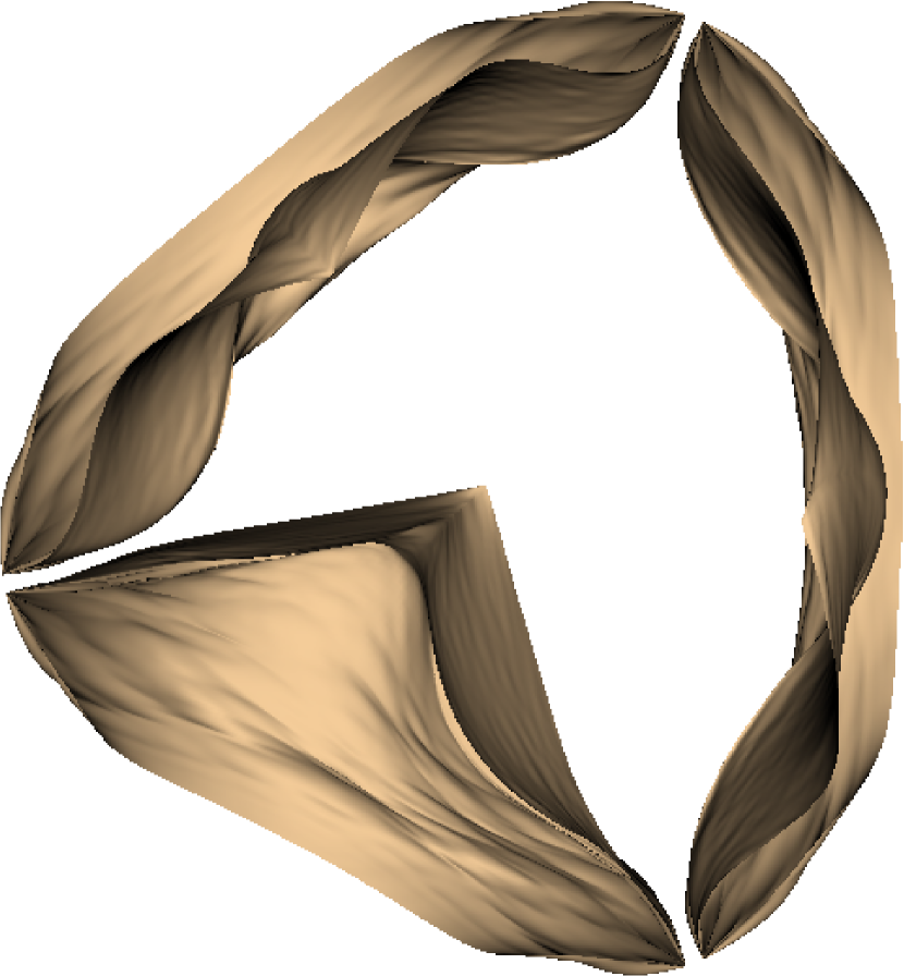
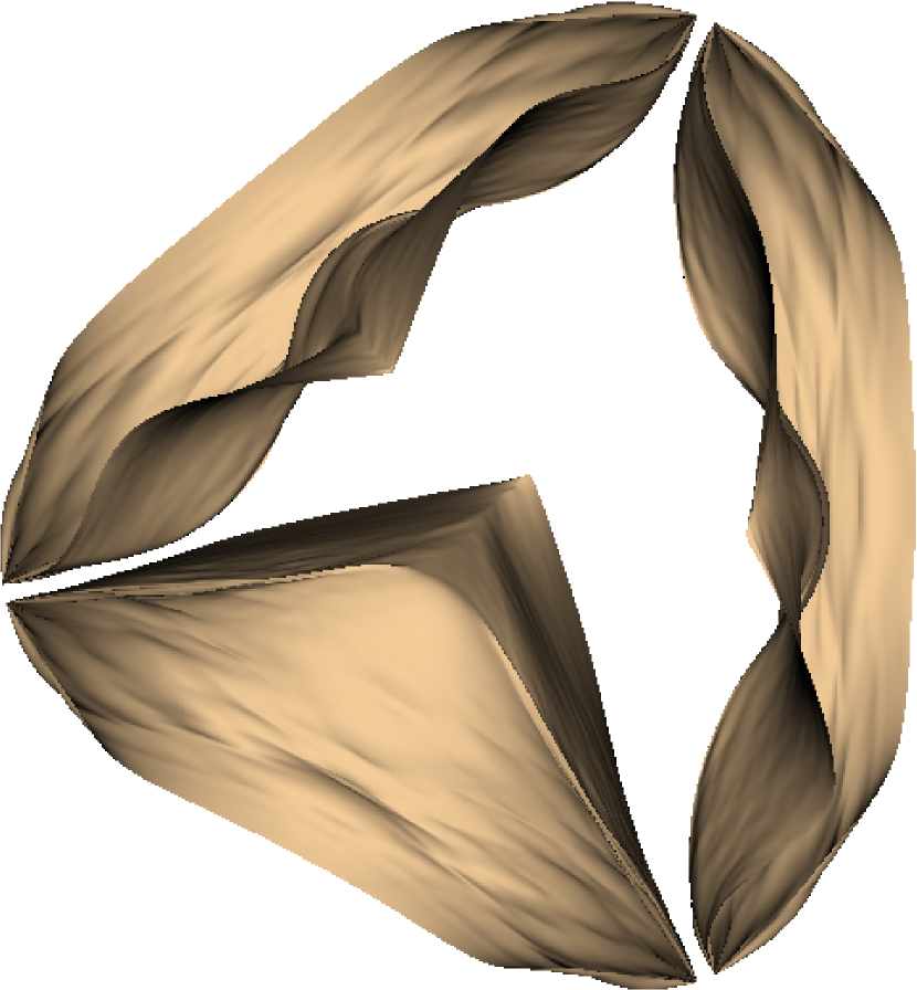
(b)

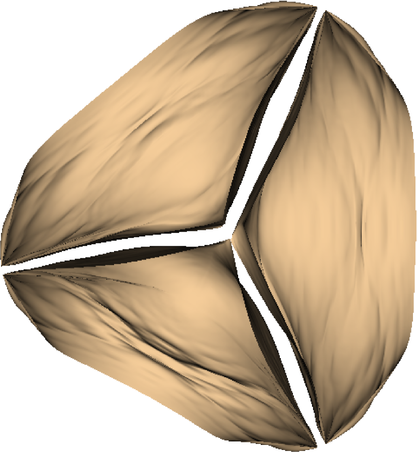
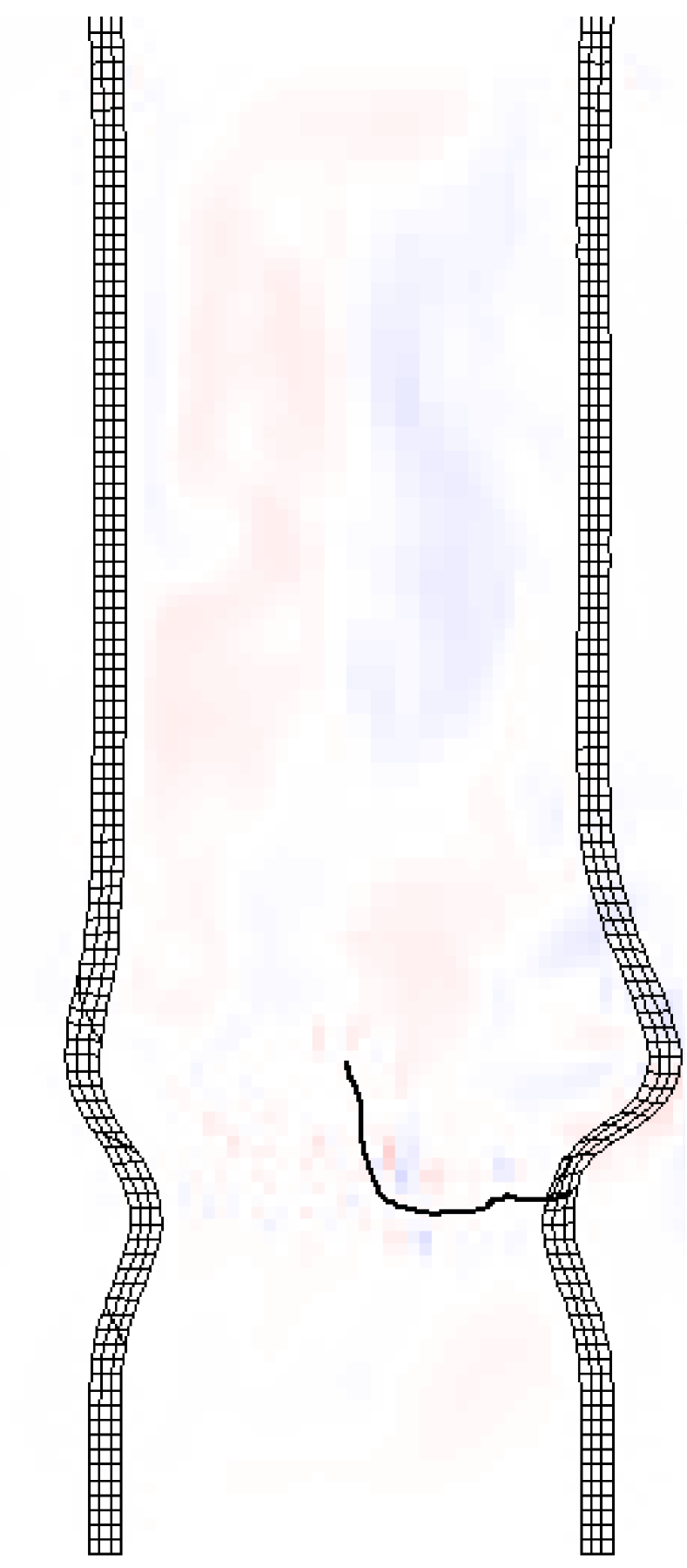
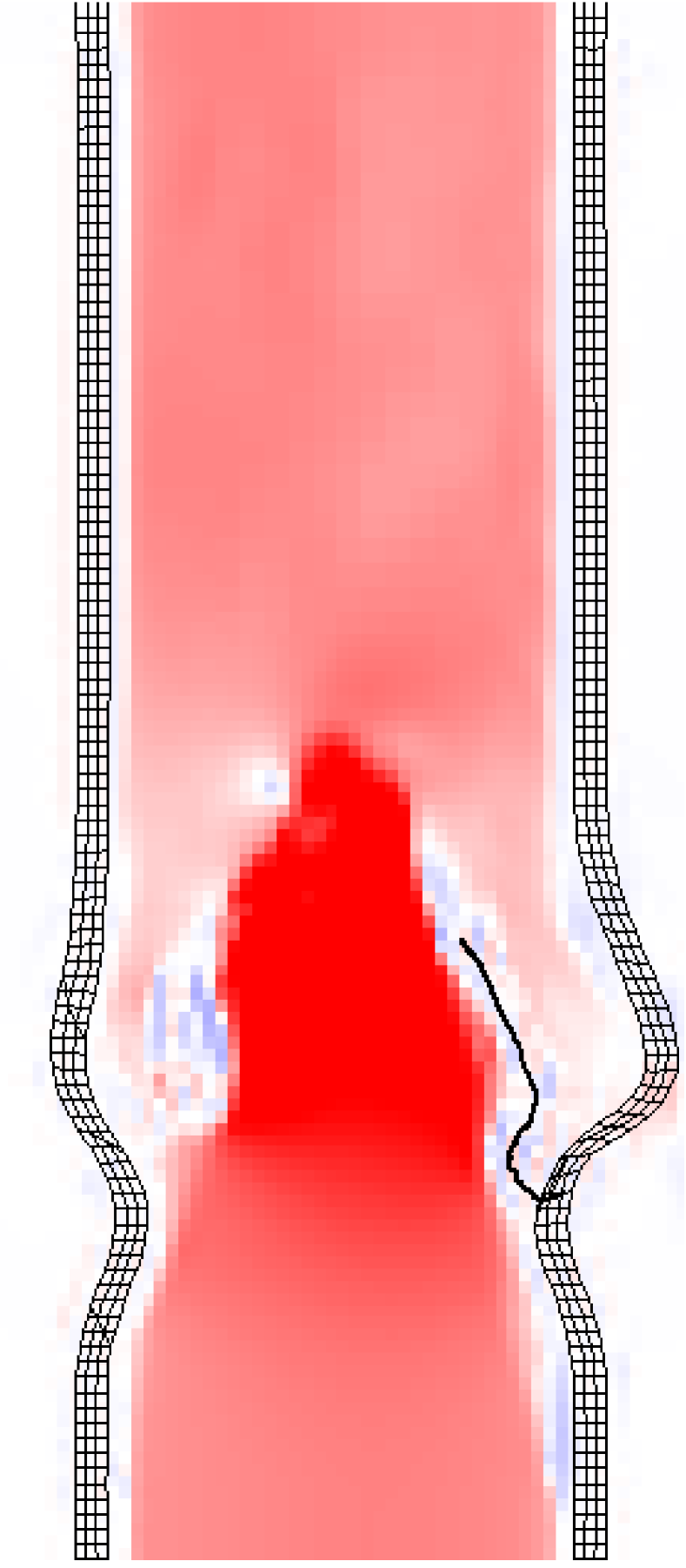
(c)

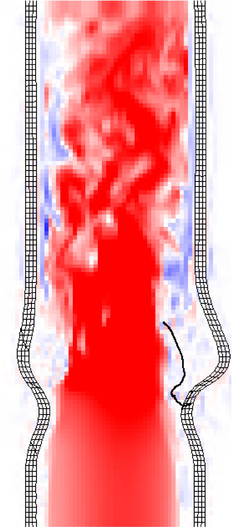
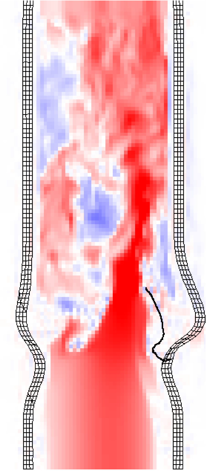
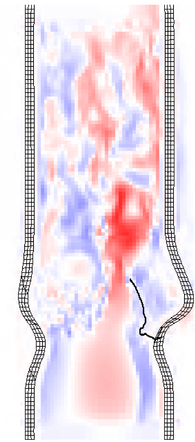
(d)

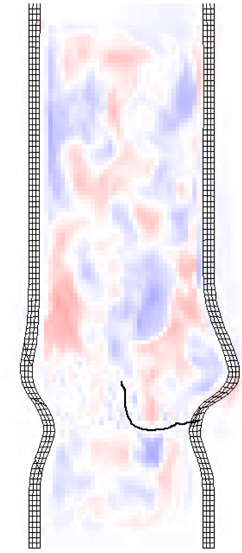
\psfragscanon\psfrag{s03}[t][t]{\color[rgb]{0,0,0}\begin{tabular}[]{c}Time (s)\end{tabular}}\psfrag{s04}[b][b]{\color[rgb]{0,0,0}\begin{tabular}[]{c}Flow Rate (ml/s)\end{tabular}}\psfrag{x01}[t][t]{1}\psfrag{x02}[t][t]{1.5}\psfrag{x03}[t][t]{2}\psfrag{x04}[t][t]{2.5}\psfrag{x05}[t][t]{3}\psfrag{x06}[t][t]{3.5}\psfrag{x07}[t][t]{4}\psfrag{v01}[r][r]{-200}\psfrag{v02}[r][r]{-100}\psfrag{v03}[r][r]{0}\psfrag{v04}[r][r]{100}\psfrag{v05}[r][r]{200}\psfrag{v06}[r][r]{300}\psfrag{v07}[r][r]{400}\psfrag{v08}[r][r]{500}\psfrag{v09}[r][r]{600}\psfrag{v10}[r][r]{700}\includegraphics{flow_open_close_asym.eps}

(e)

Figure 14: Valve leaflet configurations during (14(a)) valve opening and (14(b)) shown at equally spaced times during the fourth simulated cardiac cycle. Panels (14(c)) and (14(d)) show the corresponding axial velocity profiles. Panel (14(e)) shows the computed flow rates, with the dashed lines indicating the times shown during valve opening and with the solid lines indicating the times shown during valve closure.

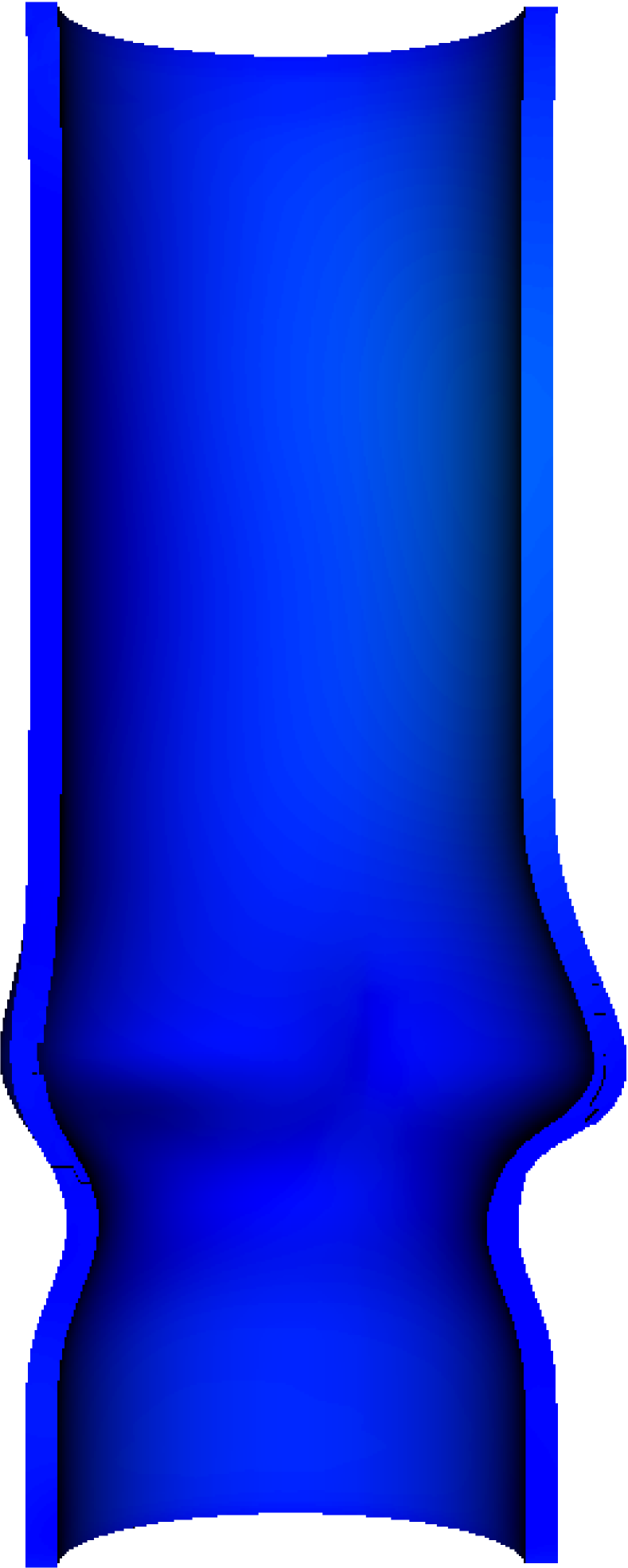
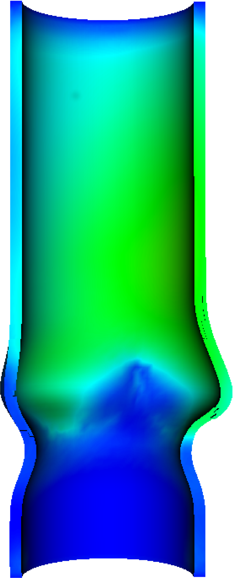
(a)

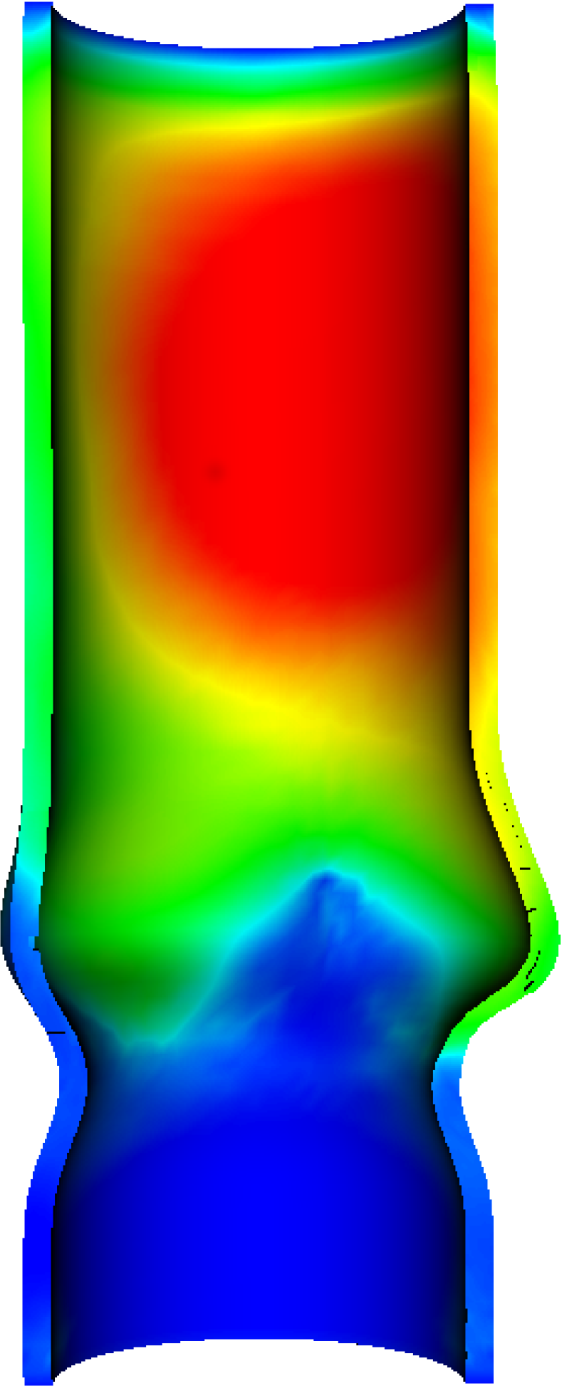
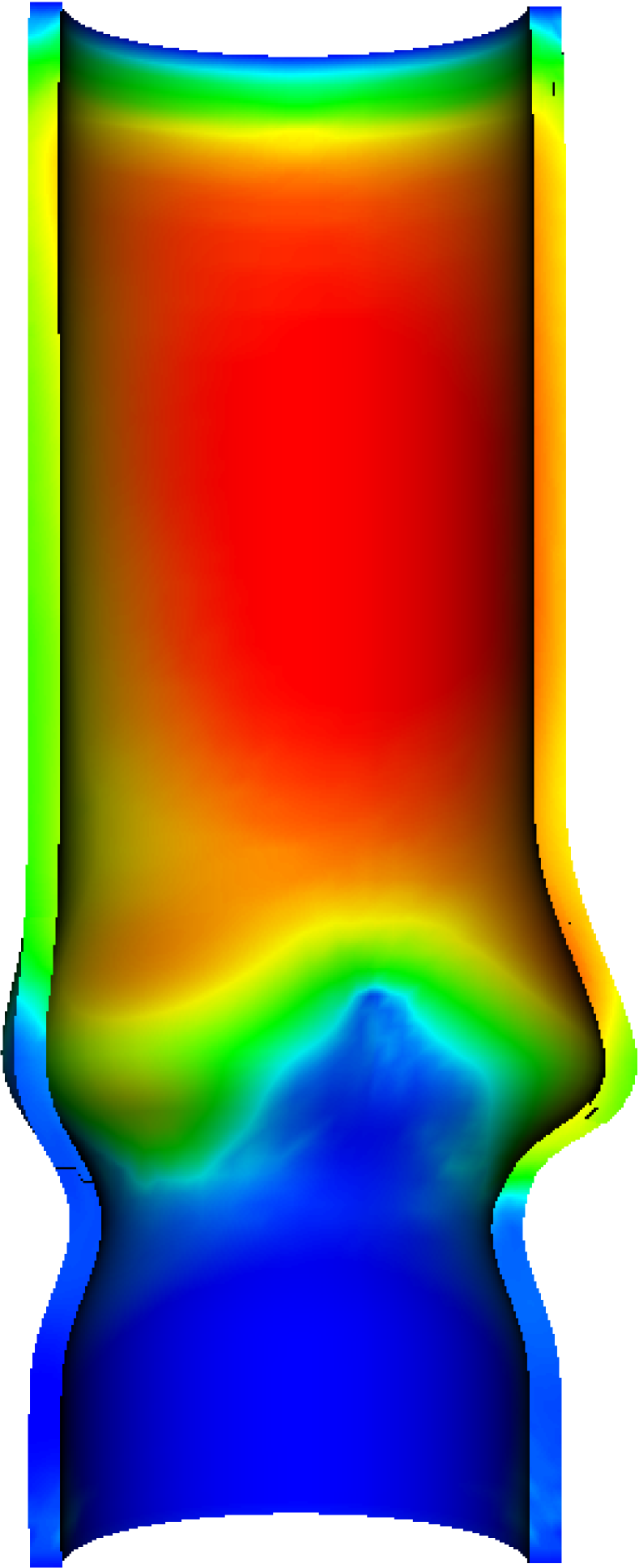
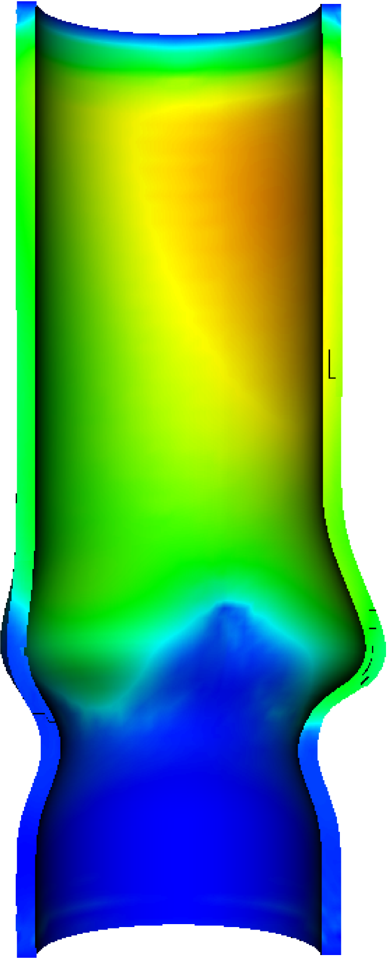
(b)

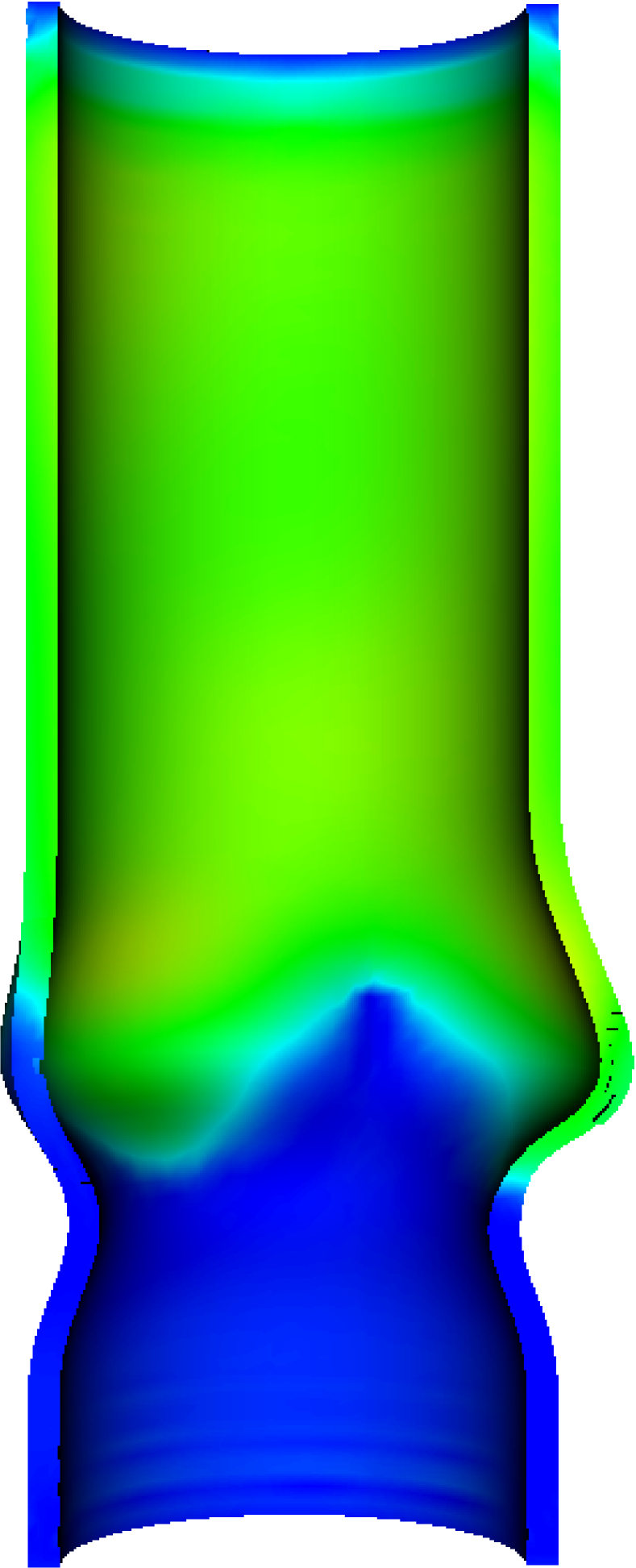
Figure 15: Displacement contours along the axial section of the asymmetric aortic root during valve opening and closure, shown at the same time instants as in fig. 14, (15(a)) during valve opening and (15(a)) during valve closure.

\psfragscanon\psfrag{s05}[t][t]{\color[rgb]{0,0,0}\begin{tabular}[]{c}Time(s)\end{tabular}}\psfrag{s06}[b][b]{\color[rgb]{0,0,0}\begin{tabular}[]{c}Displacement (mm)\end{tabular}}\psfrag{s10}{\color[rgb]{0,0,0}\begin{tabular}[]{c}\end{tabular}}\psfrag{s11}{\color[rgb]{0,0,0}\begin{tabular}[]{c}\end{tabular}}\psfrag{s12}[l][l]{\color[rgb]{0,0,0}R}\psfrag{s13}[l][l]{\color[rgb]{0,0,0}L}\psfrag{s14}[l][l]{\color[rgb]{0,0,0}N-C}\psfrag{s15}[l][l]{\color[rgb]{0,0,0}R}\psfrag{x01}[t][t]{1}\psfrag{x02}[t][t]{1.5}\psfrag{x03}[t][t]{2}\psfrag{x04}[t][t]{2.5}\psfrag{x05}[t][t]{3}\psfrag{x06}[t][t]{3.5}\psfrag{x07}[t][t]{4}\psfrag{v01}[r][r]{-0.1}\psfrag{v02}[r][r]{0}\psfrag{v03}[r][r]{0.1}\psfrag{v04}[r][r]{0.2}\psfrag{v05}[r][r]{0.3}\psfrag{v06}[r][r]{0.4}\psfrag{v07}[r][r]{0.5}\psfrag{v08}[r][r]{0.6}\psfrag{v09}[r][r]{0.7}\includegraphics{aorta_asym_dx_2.eps}

(a)

\psfragscanon\psfrag{s05}[t][t]{\color[rgb]{0,0,0}\begin{tabular}[]{c}Time(s)\end{tabular}}\psfrag{s06}[b][b]{\color[rgb]{0,0,0}\begin{tabular}[]{c}Displacement (mm)\end{tabular}}\psfrag{s10}{\color[rgb]{0,0,0}\begin{tabular}[]{c}\end{tabular}}\psfrag{s11}{\color[rgb]{0,0,0}\begin{tabular}[]{c}\end{tabular}}\psfrag{s12}[l][l]{\color[rgb]{0,0,0}R}\psfrag{s13}[l][l]{\color[rgb]{0,0,0}L}\psfrag{s14}[l][l]{\color[rgb]{0,0,0}N-C}\psfrag{s15}[l][l]{\color[rgb]{0,0,0}R}\psfrag{x01}[t][t]{1}\psfrag{x02}[t][t]{1.5}\psfrag{x03}[t][t]{2}\psfrag{x04}[t][t]{2.5}\psfrag{x05}[t][t]{3}\psfrag{x06}[t][t]{3.5}\psfrag{x07}[t][t]{4}\psfrag{v01}[r][r]{-0.1}\psfrag{v02}[r][r]{0}\psfrag{v03}[r][r]{0.1}\psfrag{v04}[r][r]{0.2}\psfrag{v05}[r][r]{0.3}\psfrag{v06}[r][r]{0.4}\psfrag{v07}[r][r]{0.5}\psfrag{v08}[r][r]{0.6}\includegraphics{commis_asym_dx_2.eps}

(b)

\psfragscanon\psfrag{s05}[t][t]{\color[rgb]{0,0,0}\begin{tabular}[]{c}Time(s)\end{tabular}}\psfrag{s06}[b][b]{\color[rgb]{0,0,0}\begin{tabular}[]{c}Displacement (mm)\end{tabular}}\psfrag{s10}{\color[rgb]{0,0,0}\begin{tabular}[]{c}\end{tabular}}\psfrag{s11}{\color[rgb]{0,0,0}\begin{tabular}[]{c}\end{tabular}}\psfrag{s12}[l][l]{\color[rgb]{0,0,0}R}\psfrag{s13}[l][l]{\color[rgb]{0,0,0}L}\psfrag{s14}[l][l]{\color[rgb]{0,0,0}N-C}\psfrag{s15}[l][l]{\color[rgb]{0,0,0}R}\psfrag{x01}[t][t]{1}\psfrag{x02}[t][t]{1.5}\psfrag{x03}[t][t]{2}\psfrag{x04}[t][t]{2.5}\psfrag{x05}[t][t]{3}\psfrag{x06}[t][t]{3.5}\psfrag{x07}[t][t]{4}\psfrag{v01}[r][r]{-0.1}\psfrag{v02}[r][r]{0}\psfrag{v03}[r][r]{0.1}\psfrag{v04}[r][r]{0.2}\psfrag{v05}[r][r]{0.3}\psfrag{v06}[r][r]{0.4}\psfrag{v07}[r][r]{0.5}\psfrag{v08}[r][r]{0.6}\includegraphics{STJ_asym_dx_2.eps}

(c)

\psfragscanon\psfrag{s05}[t][t]{\color[rgb]{0,0,0}\begin{tabular}[]{c}Time(s)\end{tabular}}\psfrag{s06}[b][b]{\color[rgb]{0,0,0}\begin{tabular}[]{c}Displacement (mm)\end{tabular}}\psfrag{s10}{\color[rgb]{0,0,0}\begin{tabular}[]{c}\end{tabular}}\psfrag{s11}{\color[rgb]{0,0,0}\begin{tabular}[]{c}\end{tabular}}\psfrag{s12}[l][l]{\color[rgb]{0,0,0}R}\psfrag{s13}[l][l]{\color[rgb]{0,0,0}L}\psfrag{s14}[l][l]{\color[rgb]{0,0,0}N-C}\psfrag{s15}[l][l]{\color[rgb]{0,0,0}R}\psfrag{x01}[t][t]{1}\psfrag{x02}[t][t]{1.5}\psfrag{x03}[t][t]{2}\psfrag{x04}[t][t]{2.5}\psfrag{x05}[t][t]{3}\psfrag{x06}[t][t]{3.5}\psfrag{x07}[t][t]{4}\psfrag{v01}[r][r]{-0.05}\psfrag{v02}[r][r]{0}\psfrag{v03}[r][r]{0.05}\psfrag{v04}[r][r]{0.1}\psfrag{v05}[r][r]{0.15}\psfrag{v06}[r][r]{0.2}\psfrag{v07}[r][r]{0.25}\psfrag{v08}[r][r]{0.3}\psfrag{v09}[r][r]{0.35}\psfrag{v10}[r][r]{0.4}\psfrag{v11}[r][r]{0.45}\includegraphics{sinus_asym_dx_2.eps}

(d)

Figure 16: Displacements of the asymmetric aortic root model at four locations: (16(a)) the straight portion of the aorta; (16(b)) just above one of the commissures; (16(c)) the sinotubular junction; and (16(d)) the middle of the sinus.

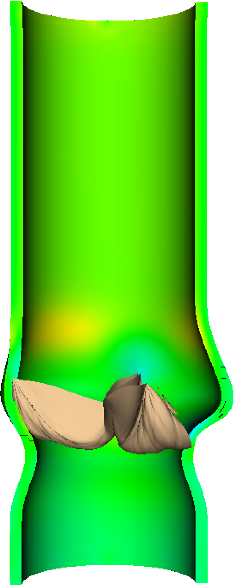
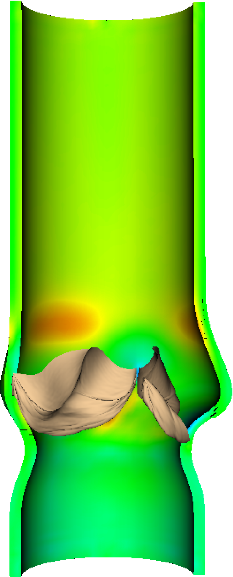
(a)

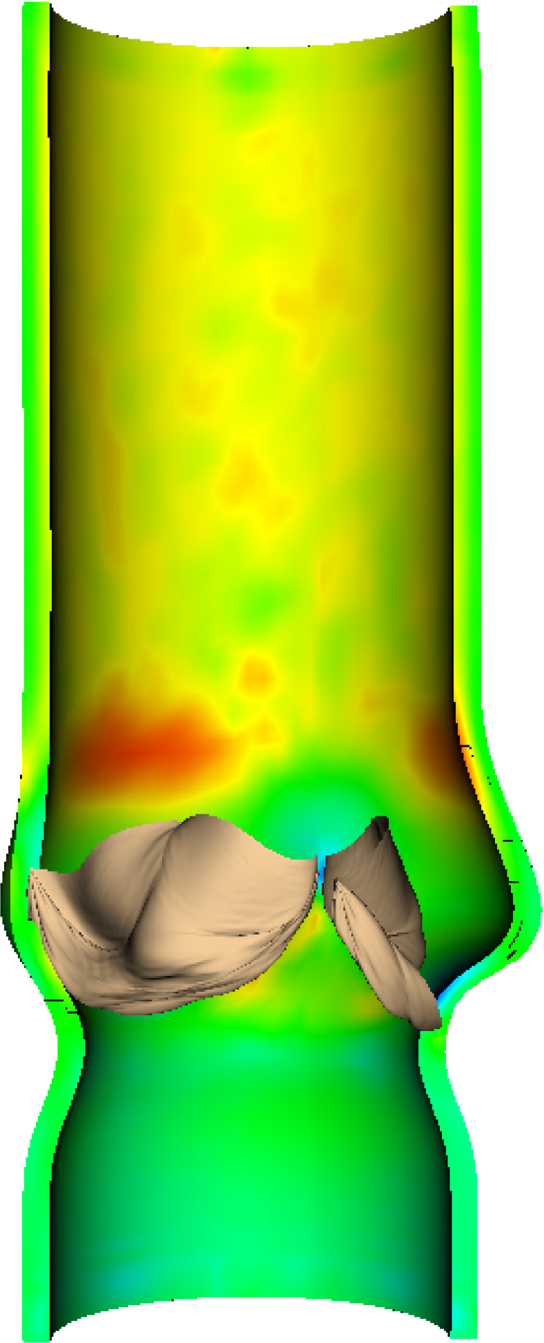
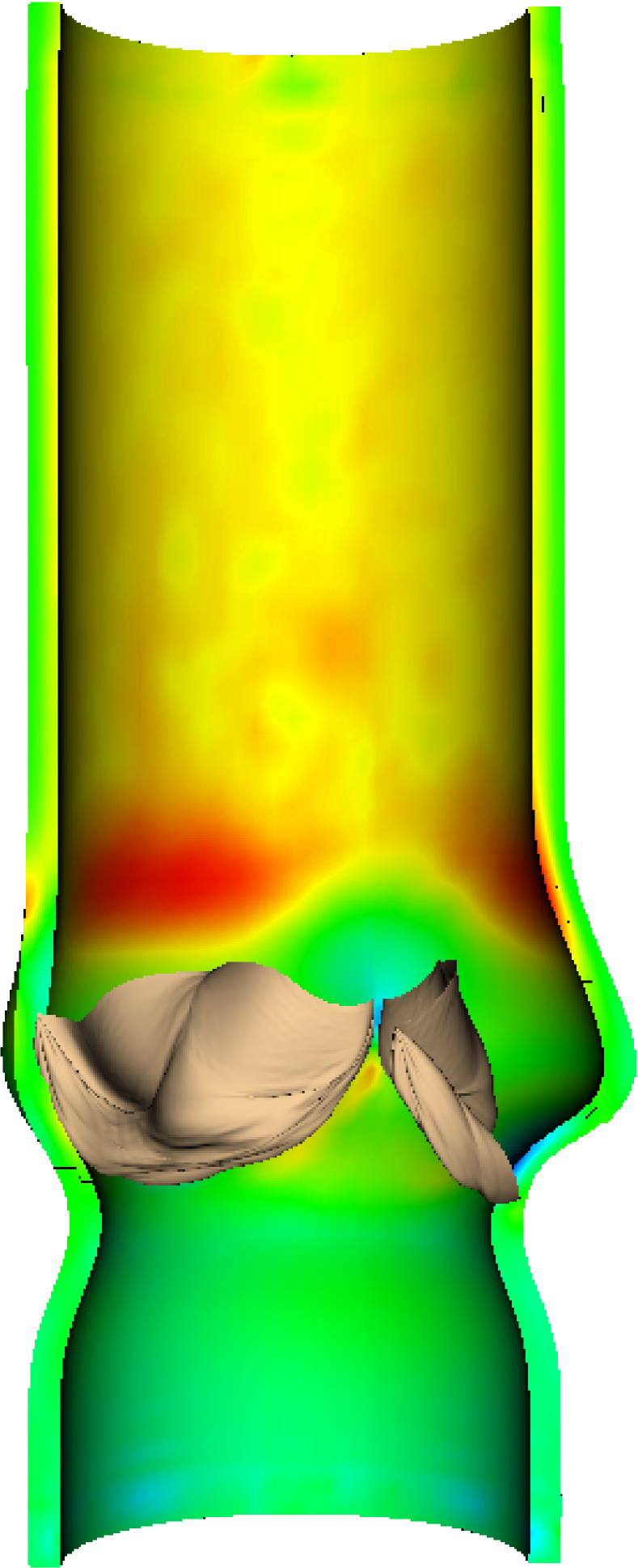
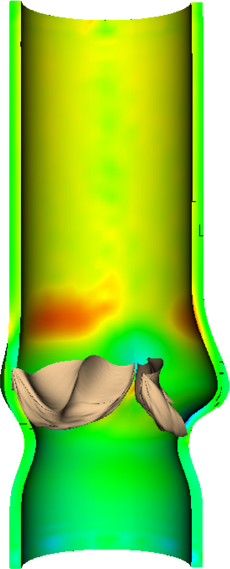
(b)

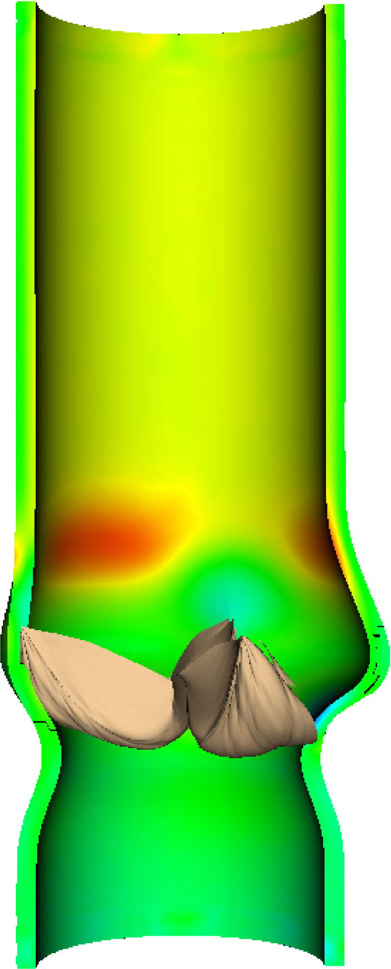
Figure 17: Maximum principal stress contours along the axial section of the asymmetric aortic root during valve opening and closure, shown at the same time instants as in fig. 14, (17(a)) during valve opening and (17(b)) during valve closure.

\psfragscanon\psfrag{s05}[t][t]{\color[rgb]{0,0,0}\begin{tabular}[]{c}Time(s)\end{tabular}}\psfrag{s06}[b][b]{\color[rgb]{0,0,0}\begin{tabular}[]{c}Max Principal Stress (kPa)\end{tabular}}\psfrag{s10}{\color[rgb]{0,0,0}\begin{tabular}[]{c}\end{tabular}}\psfrag{s11}{\color[rgb]{0,0,0}\begin{tabular}[]{c}\end{tabular}}\psfrag{s12}[l][l]{\color[rgb]{0,0,0}R}\psfrag{s13}[l][l]{\color[rgb]{0,0,0}L}\psfrag{s14}[l][l]{\color[rgb]{0,0,0}N-C}\psfrag{s15}[l][l]{\color[rgb]{0,0,0}R}\psfrag{x01}[t][t]{1}\psfrag{x02}[t][t]{1.5}\psfrag{x03}[t][t]{2}\psfrag{x04}[t][t]{2.5}\psfrag{x05}[t][t]{3}\psfrag{x06}[t][t]{3.5}\psfrag{x07}[t][t]{4}\psfrag{v01}[r][r]{60}\psfrag{v02}[r][r]{70}\psfrag{v03}[r][r]{80}\psfrag{v04}[r][r]{90}\psfrag{v05}[r][r]{100}\psfrag{v06}[r][r]{110}\psfrag{v07}[r][r]{120}\psfrag{v08}[r][r]{130}\psfrag{v09}[r][r]{140}\includegraphics{aorta_sp1.eps}

(a)

\psfragscanon\psfrag{s05}[t][t]{\color[rgb]{0,0,0}\begin{tabular}[]{c}Time(s)\end{tabular}}\psfrag{s06}[b][b]{\color[rgb]{0,0,0}\begin{tabular}[]{c}Max Principal Stress (kPa)\end{tabular}}\psfrag{s10}{\color[rgb]{0,0,0}\begin{tabular}[]{c}\end{tabular}}\psfrag{s11}{\color[rgb]{0,0,0}\begin{tabular}[]{c}\end{tabular}}\psfrag{s12}[l][l]{\color[rgb]{0,0,0}R}\psfrag{s13}[l][l]{\color[rgb]{0,0,0}L}\psfrag{s14}[l][l]{\color[rgb]{0,0,0}N-C}\psfrag{s15}[l][l]{\color[rgb]{0,0,0}R}\psfrag{x01}[t][t]{1}\psfrag{x02}[t][t]{1.5}\psfrag{x03}[t][t]{2}\psfrag{x04}[t][t]{2.5}\psfrag{x05}[t][t]{3}\psfrag{x06}[t][t]{3.5}\psfrag{x07}[t][t]{4}\psfrag{v01}[r][r]{60}\psfrag{v02}[r][r]{70}\psfrag{v03}[r][r]{80}\psfrag{v04}[r][r]{90}\psfrag{v05}[r][r]{100}\psfrag{v06}[r][r]{110}\psfrag{v07}[r][r]{120}\psfrag{v08}[r][r]{130}\psfrag{v09}[r][r]{140}\psfrag{v10}[r][r]{150}\includegraphics{Commissura_sp1.eps}

(b)

\psfragscanon\psfrag{s05}[t][t]{\color[rgb]{0,0,0}\begin{tabular}[]{c}Time(s)\end{tabular}}\psfrag{s06}[b][b]{\color[rgb]{0,0,0}\begin{tabular}[]{c}Max Principal Stress (kPa)\end{tabular}}\psfrag{s10}{\color[rgb]{0,0,0}\begin{tabular}[]{c}\end{tabular}}\psfrag{s11}{\color[rgb]{0,0,0}\begin{tabular}[]{c}\end{tabular}}\psfrag{s12}[l][l]{\color[rgb]{0,0,0}R}\psfrag{s13}[l][l]{\color[rgb]{0,0,0}L}\psfrag{s14}[l][l]{\color[rgb]{0,0,0}N-C}\psfrag{s15}[l][l]{\color[rgb]{0,0,0}R}\psfrag{x01}[t][t]{1}\psfrag{x02}[t][t]{1.5}\psfrag{x03}[t][t]{2}\psfrag{x04}[t][t]{2.5}\psfrag{x05}[t][t]{3}\psfrag{x06}[t][t]{3.5}\psfrag{x07}[t][t]{4}\psfrag{v01}[r][r]{80}\psfrag{v02}[r][r]{100}\psfrag{v03}[r][r]{120}\psfrag{v04}[r][r]{140}\psfrag{v05}[r][r]{160}\psfrag{v06}[r][r]{180}\psfrag{v07}[r][r]{200}\includegraphics{SJT_sp1.eps}

(c)

\psfragscanon\psfrag{s05}[t][t]{\color[rgb]{0,0,0}\begin{tabular}[]{c}Time(s)\end{tabular}}\psfrag{s06}[b][b]{\color[rgb]{0,0,0}\begin{tabular}[]{c}Max Principal Stress (kPa)\end{tabular}}\psfrag{s10}{\color[rgb]{0,0,0}\begin{tabular}[]{c}\end{tabular}}\psfrag{s11}{\color[rgb]{0,0,0}\begin{tabular}[]{c}\end{tabular}}\psfrag{s12}[l][l]{\color[rgb]{0,0,0}R}\psfrag{s13}[l][l]{\color[rgb]{0,0,0}L}\psfrag{s14}[l][l]{\color[rgb]{0,0,0}N-C}\psfrag{s15}[l][l]{\color[rgb]{0,0,0}R}\psfrag{x01}[t][t]{1}\psfrag{x02}[t][t]{1.5}\psfrag{x03}[t][t]{2}\psfrag{x04}[t][t]{2.5}\psfrag{x05}[t][t]{3}\psfrag{x06}[t][t]{3.5}\psfrag{x07}[t][t]{4}\psfrag{v01}[r][r]{15}\psfrag{v02}[r][r]{20}\psfrag{v03}[r][r]{25}\psfrag{v04}[r][r]{30}\psfrag{v05}[r][r]{35}\psfrag{v06}[r][r]{40}\psfrag{v07}[r][r]{45}\psfrag{v08}[r][r]{50}\includegraphics{sinus_sp1.eps}

(d)

Figure 18: Maximum principal stress of the asymmetric aorta over the cycles that reached periodic steady state at four locations: (18(a)) the straight portion of the aorta; (18(b)) just above the commissures; (18(c)) the sinotubular junction; and (18(d)) the middle of sinus.

Similar fluid-structure interaction simulations are performed using the asymmetric model using only the coarser Cartesian grid spacing of $h=0.78125~{}\text{mm}$. Fig. 13 shows the prescribed left ventricular driving pressure and the computed aortic pressure along with the computed flow rate generated by the model. Peak flow rate in this model is 581 ml/s, which is reduced compared to the symmetric studies and is within 5% of the subject-specific peak flow rate of 560 ml/s murgo1980 . Stroke volume and cardiac output are 95.1 ml and 6.46 l/min, respectively, which are both within 6% of the respective clinical values of 100 ml and 6.8 l/m murgo1980 .

The details of the valve kinematics are also different with the asymmetric model, but the model is still able to capture the leaflets being pushed back, the flow inversion, the vortices in the sinuses, and the valve closure, which does not allow regurgitation during diastole; see figs. 14.

Overall, the distribution of the displacements appeared similar to the symmetric case, with the ascending aorta and the sinotubular junction moving more than the rest of the aortic root, as shown in fig. 15; however, tracking the displacements over time at specific locations for the right, left, and noncoronary sinus shows that the left sinus moves 20% less than the right sinus and 10% less than the noncoronary sinus. In addition, fig. 15 shows that the left sector of the aorta maintains a restricted motion compared to the right and noncoronary sectors of the aorta. This behavior can be observed also in the aorta in which the radial pulsation ranges from 1.9% for the left sector of the aorta, to 3.9% for the right sector of the aorta. The average displacement amplitude in the sinotubular junction is 0.49 mm for the right and noncoronary sinus and 0.36 mm for the left sinus. In the ascending aorta, the average displacement amplitude is 0.54 mm in the right and noncoronary portion and 0.34 mm in the left portion of the aortic wall.

The global distribution of the maximum principal stress was similar in the symmetric and asymmetric models, with the maximum stress being concentrated at the sinotubular junction, in correspondence with the sinuses; see fig. 15. Differences in the maximum principal stress at the same locations for the right, left, and noncoronary sinus, are more complex. Whereas the maximum principal stress in the aorta is essentially independent of the sector of the geometry considered, there are large differences in the stress computed in the left, right, and noncoronary sinus, especially in the cusp of the sinuses and in the sinotubular junction. Peak maximum principal stress for the sinotubular junction is 180 kPa, a value comparable to the 220 kPa value obtained by Conti et al. conti2010 . Peak principal stresses in the sinuses, evaluated at the cusp, resulted smaller in magnitude than the values reported by Grande-Allen et al. grande1998 , although the relative differences between the stresses in the sinuses is similar to those observed in that work.

4 Discussion

In this work, previous IB models of aortic valve dynamics griffith2009 ; griffith2012 are substantially extended by incorporating a deformable model of the aortic sinuses and ascending aorta. This extended model is thereby able to more closely replicate the complex in vivo dynamics of the real aortic root. As before, the dynamic analyses of the aortic valve included four complete cardiac cycles, including a single initialization cycle, which are shown to be sufficient to yield essentially periodic results. As in previous IB models of aortic valve dynamics griffith2009 ; griffith2012 , key hemodynamic parameters, including aortic pressure, maximum flow rate, cardiac output, and stroke volume, are in reasonable agreement with physiological ranges driscol1965 ; westerhof2010 and are also in good agreement with the patient-specific data murgo1980 used to fit the Windkessel model stergiopulos1999 employed in this study. Further, grid convergence results demonstrate for the first time that the IB method is able to yield essentially grid-resolved bulk flow parameters and vessel deformations at practical grid spacings.

Many strategies have been developed to determine the zero-pressure geometry of blood vessels gee2009 ; alastrue2010 ; vavourakis2011 ; bols2012 ; dePutter2007 ; sellier2011 . Indeed, medical images of arteries always provide the vessel geometry in a loaded configuration. It is known, however, that using the imaged geometry as the reference geometry of the vessel underestimates the amount of strain present in the blood vessel dePutter2007 . Among the approaches developed to estimate the zero-pressure geometry of blood vessels, we chose an iterative backward displacement approach, as described by Bols et al. bols2012 and by Sellier sellier2011 . Iterative approaches based on geometric considerations are straightforward to implement and can be applied to a variety of problems and solvers because they require minimal implementation effort. In this work, the backward displacement analysis was implemented in ABAQUS and converged to a zero-pressure geometry that, when loaded, yielded a deformed configuration that is in good agreement with the initially prescribed loaded geometry; see figs. 3–5. However, the deflated geometry is quite different from the configuration assumed by a deflated aortic root harvested from a body; see fig. 3. This is a drawback of these methods, as shown also in a recent study by Wittek et al. wittek2013 , in which the unloaded configuration of the aorta is different from an unloaded aorta harvested from a body. This mismatch could be the result of many factors, such as the choice of the boundary conditions or the need for adding the residual stress to balance the level of stress within the aortic wall fung1991 . We expect that the addition of residual stress estimates, planned in future work, will reduce the mismatch between the deflated geometry computed and the deflated aortic root observed in vivo.

Interestingly, the addition of a compliant aortic wall did not substantially alter the global hemodynamic parameters previously determined by a noncompliant IB aortic root model griffith2012 . In general, we observed a slight increase in the maximum flow rate as compared to the noncompliant model, whereas changes in other global flow parameters were relatively minor. This finding might suggest that our vessel wall model is overly stiff despite our use of a constitutive model fit to biaxial tensile test data from human aortic tissues samples. In contrast, we observed that using a compliant aorta affected more clearly the dynamics of valve leaflet closure. Figs. 7(7(b)) and 8(8(b)) show the flow inversion and the distension in the sinus, which collects fluid during systolic ejection, and the elastic recoil of the sinus, which pushes down on the leaflet during closure. The addition of this mechanism made the model substantially more robust. Specifically, we found that the rigid aortic root model required the valve leaflet properties to be very carefully tuned in order for the model to remain competent throughout the cardiac cycle. This is in clear contrast to the present compliant aortic root model, which yields a competent valve for a relatively broad range of leaflet parameters.

Similar model predictions were obtained for both Cartesian grid spacings used in this study. We observed hemodynamic values that were within 5% of the clinical values reported by Murgo et al. murgo1980 except for the peak flow rate, which was within 5% of the values reported by Murgo et al. on the coarser Cartesian grid and within 15% on the finer grid. Cardiac output and stroke volume were both in very good agreement with the clinical data, within 4% on the coarser Cartesian grid, and within 1% on the finer grid. In addition, the pulsatile radius, a quantity used to measure aortic stiffness, was also shown to be in relatively good agreement with literature values in both cases humphrey2002 .

To make the description of the aortic root dynamics more realistic, we modified the aortic geometry and the leaflets configuration to replicate the physiological asymmetry of the sinuses and the leaflets. Previous work by Grande-Allen et al. grande1998 and by Conti et al. conti2010 showed that the use of a realistic geometry in FE and computational fluid dynamics simulations of the aortic root yields more accurate results for the stress distribution along the sinuses. We based our asymmetric aortic root geometries on the inter-commissures distances reported by Berdajs berdajs2002 . Overall, the bulk flow parameters were closer to the original values reported by Murgo murgo1980 than the corresponding values obtained with a symmetric model for the same level of grid refinement. These results suggest that the use of a more realistic geometry could yield more accurate estimates of key hemodynamic quantities. Structural stresses generated by the immersed boundary model were also in good agreement with the stresses reported by Conti et al. conti2010 . Moreover, the level of stress and the displacement of the right and in the noncoronary sectors of the aortic root, but not in the left sector of the aortic root, were similar in the symmetric and the asymmetric case; see figs. 10 and 16.

Leaflet dynamics for the symmetric aortic valve are shown in figs. 7 and 8, and leaflet dynamics for the asymmetric aortic valve are shown instead in fig. 14. It is possible to see, however, that in the asymmetric model, the left coronary leaflet starts closing before the other two leaflets, thus bending the flow profile in the aortic tract; see fig. 14(14(d)). Because the aortic root model is asymmetric, there is no reason to expect that the dynamics of the three leaflets will be identical. We plan to study this asymmetry in the leaflet kinematics more carefully in the context of a more geometrically realistic model of the aortic root that accounts for the curvature of the real aortic root and ascending aorta.

4.1 Limitations and Future Work

Work is underway to address some of the limitations of these models. As described previously, our present models do not account for the curved geometry of the aortic root, or for the residual stresses present in real arterial vessels. We specifically aim to incorporate a description of residual stresses and realistic medical imaging-derived anatomic geometries into our IB models. Further, the present models use an isotropic model of the aortic sinuses and ascending aorta. Although the experimental data that were used to fit this model show an essentially isotropic material response, it is known that real aortic tissues have a well-defined collagen fiber structure with an anisotropic material response. We also aim to incorporate a more realistic hyperelastic model of the aortic wall that accounts for families of collagen fibers gasser2006 as well as experimentally constrained models of the elasticity of the aortic valve leaflets may-newman-2009 . Further, it is now well known that the valve leaflets are in fact layered structures sacks2007 . These details are not accounted for in the present model, and we anticipate that including them in future work will require an important extension of the methods presented in this study. Specifically, because the valve leaflets are thin elastic structures, we expect that using realistic hyperelastic continuum models to describe the mechanics of the valve leaflets will require adopting a nonlinear shell formulation. To our knowledge, continuum shell models have not yet been widely used within the framework of the IB method, and we anticipate additional computational research will be required to implement these types of formulations into our IB simulation framework.

Another limitation of this work is the long run times required by these simulations. Because of the small time step sizes required by the present algorithm, each cardiac cycle required 50,000 or more time steps, requiring on the order of one day per cycle on 32–64 cores of a modern high-performance computing (HPC) cluster for the coarse simulations and on the order of one week per cycle for the fine-grid simulations. We are currently working to develop effective multigrid solvers for stable implicit time stepping schemes for the IB method RDGuyXX-gmgiib . These methods promise to allow for substantially larger time step sizes as well as shorter run times at current grid resolutions. They could also enable higher resolution simulations that promise to resolve the fine-scale details of the dynamics of the aortic root.

5 Conclusions

This work has presented new fluid-structure interaction models of the aortic root that extend earlier IB models of the aortic valve by incorporating a finite-strain model of the aortic root that uses a constitutive model fit to tensile test data obtained from human aortic root tissue specimens. The models capture both the complex fluid dynamics of the flow and the finite deformations of the vessel wall, and they yield results that are in good agreement with the clinical data that were used to fit the circulation model used in this study, as well as to physiological data in the research literature. In addition, a grid convergence study demonstrates that nearly grid converged results are obtained at practical spatial resolutions, although yet higher spatial resolution is needed to obtain fully resolved simulation results. Finally, by comparing the dynamics of symmetric and asymmetric aortic root models, we find that the asymmetric model appears to yield a more accurate description of both the bulk flow properties and also the aortic wall mechanics.

- (1) Alastrué, V., Garía, A., Peña, E., Rodríguez, J., Martínez, M., Doblaré, M.: Numerical framework for patient-specific computational modelling of vascular tissue. Int J Numer Method Biomed Eng 26(1), 35–51 (2010)
- (2) Alastrué, V., Peña, E., Martínez, M.Á., Doblaré, M.: Assessing the use of the “opening angle method” to enforce residual stresses in patient-specific arteries. Ann Biomed Eng 35(10), 1821–1837 (2007)
- (3) Azadani, A.N., Chitsaz, S., Matthews, P.B., Jaussaud, N., Leung, J., Tsinman, T., Ge, L., Tseng, E.E.: Comparison of mechanical properties of human ascending aorta and aortic sinuses. Ann Thorac Surg 93(1), 87–94 (2012)
- (4) Bellhouse, B.J., Bellhouse, F.H.: Mechanism of closure of the aortic valve. Nature 217, 86–87 (1968)
- (5) Berdajs, D., Lajos, P., Turina, M.: The anatomy of the aortic root. Vascular 10(4), 320–327 (2002)
- (6) Bols, J., Degroote, J., Trachet, B., Verhegghe, B., Segers, P., Vierendeels, J.: A computational method to assess in vivo stresses and unloaded configuration of patient-specific blood vessels. J Comput Appl Math (2012)
- (7) Bonow, R.O., Carabello, B.A., Chatterjee, K., de Leon, A.C., Faxon, D.P., Freed, M.D., Gaasch, W.H., Lytle, B.W., Nishimura, R.A., O’Gara, P.T., O’Rourke, R.A., Otto, C.M., Shah, P.M., Shanewise, J.S.: ACC/AHA 2006 guidelines for the management of patients with valvular heart disease. Circulation 114(5), E84–E231 (2006)
- (8) Borazjani, I.: Fluid–structure interaction, immersed boundary-finite element method simulations of bio-prosthetic heart valves. Comput Meth Appl Mech Eng 257, 103–116 (2013)
- (9) Borazjani, I., Ge, L., Sotiropoulos, F.: Curvilinear immersed boundary method for simulating fluid structure interaction with complex 3D rigid bodies. J Comput Phys 227(16), 7587–7620 (2008)
- (10) Cai, M., Nonaka, A., Bell, J., Griffith, B., Donev, A.: Efficient variable-coefficient finite-volume Stokes solvers Submitted
- (11) Cardamone, L., Valentín, A., Eberth, J.F., Humphrey, J.D.: Origin of axial prestretch and residual stress in arteries. Biomech Model Mechanobiol 8(6), 431–446 (2009)
- (12) Carr, J.A., Savage, E.B.: Aortic valve repair for aortic insufficiency in adults: A contemporary review and comparison with replacement techniques. Eur J Cardio Thorac Surg 25(1), 6–15 (2005)
- (13) Cheng, A., Dagum, P., Miller, D.C.: Aortic root dynamics and surgery: from craft to science. Phil Trans R Soc B 362(1484), 1407–1419 (2007)
- (14) Cheng, R., Lai, Y.G., Chandran, K.B.: Three-dimensional fluid-structure interaction simulation of bileaflet mechanical heart valve flow dynamics. Ann Biomed Eng 32(11), 1471–1483 (2004)
- (15) Conti, C.A., Votta, E., Della Corte, A., Del Viscovo, L., Bancone, C., Cotrufo, M., Redaelli, A.: Dynamic finite element analysis of the aortic root from mri-derived parameters. Med Eng Phys 32(2), 212–221 (2010)
- (16) Creane, A., Kelly, D.J., Lally, C.: Patient specific computational modeling in cardiovascular mechanics. In: B.C. Lopez, E. Peña (eds.) Patient-Specific Computational Modeling, pp. 61–79. Springer (2012)
- (17) Croft, L.R., Mofrad, M.R.K.: Computational modeling of aortic heart valves. In: S. De, F. Guilak, M.R.K. Mofrad (eds.) Computational Modeling in Biomechanics, pp. 221–252. Springer (2010)
- (18) Crosetto, P., Reymond, P., Deparis, S., Kontaxakis, D., Stergiopulos, N., Quarteroni, A.: Fluid–structure interaction simulation of aortic blood flow. Comput Fluid 43(1), 46–57 (2011)
- (19) Dagum, P., Green, G.R., Nistal, F.J., Daughteres, G.T., Timek, T.A., Foppiano, L.E., Bolger, A.F., Ingels, N.B., Miller, D.C.: Deformational dynamics of the aortic root: modes and physiologic determinants. Circulation 100(2), II54–II62 (1999)
- (20) De Hart, J., Baaijens, F.P.T., Peters, G.W.M., Schreurs, P.J.G.: A computational fluid-structure interaction analysis of a fiber-reinforced stentless aortic valve. J Biomech 36(5), 699–712 (2003)
- (21) de Putter, S., Wolters, B.J.B.M., Rutten, M.C.M., Breeuwer, M., Gerritsen, F.A., van de Vosse, F.N.: Patient-specific initial wall stress in abdominal aortic aneurysms with a backward incremental method. J Biomech 40(5), 1081 – 1090 (2007)
- (22) Delfino, A., Stergiopulos, N., Moore, J.E., Meister, J.J.: Residual strain effects on the stress field in a thick wall finite element model of the human carotid bifurcation. J Biomech 30(8), 777–786 (1997)
- (23) Driscol, T.E., Eckstein, R.W.: Systolic pressure gradients across the aortic valve and in the ascending aorta. Am J Physiol 209(3), 557–563 (1965)
- (24) Dumont, K., Stijnen, J.M.A., Vierendeels, J., Van De Vosse, F.N., Verdonck, P.R.: Validation of a fluid–structure interaction model of a heart valve using the dynamic mesh method in fluent. Comput Meth Biomech Biomed Eng 7(3), 139–146 (2004)
- (25) Fai, T.G., Griffith, B.E., Mori, Y., Peskin, C.S.: Immersed boundary method for variable viscosity and variable density problems using fast linear solvers. I: Numerical method and results. SIAM J Sci Comput 35(5), B1132––B1161 (2013)
- (26) Freeman, R.V., Otto, C.M.: Spectrum of calcific aortic valve disease: Pathogenesis, disease progression, and treatment strategies. Circulation 111(24), 3316–3326 (2005)
- (27) Fung, Y.C.: What principle governs the stress distribution in living organs? In: Y.C. Fung, E. Fukada, J. Wang (eds.) Biomechanics in China, Japan and USA. Science Press (1983)
- (28) Fung, Y.C.: What are the residual stresses doing in our blood vessels? Ann Biomed Eng 19(3), 237–249 (1991)
- (29) Gao, H., Wang, H.M., Berry, C., Luo, X.Y., Griffith, B.E.: Quasi-static image-based immersed boundary-finite element model of left ventricle under diastolic loading. Int J Numer Meth Biomed Eng 30(11), 1199–1222 (2014)
- (30) Gasser, T.C., Ogden, R.W., Holzapfel, G.A.: Hyperelastic modelling of arterial layers with distributed collagen fibre orientations. J R Soc Interface 3(6), 15–35 (2006)
- (31) Gee, M.W., Reeps, C., Eckstein, H.H., Wall, W.A.: Prestressing in finite deformation abdominal aortic aneurysm simulation. J Biomech 42(11), 1732–1739 (2009)
- (32) Govindjee, S., Mihalic, P.A.: Computational methods for inverse deformations in quasi-incompressible finite elasticity. Int J Numer Method Eng 43(5), 821–838 (1998)
- (33) Grande, K.J., Cochran, R.P., Reinhall, P.G., Kunzelman, K.S.: Stress variations in the human aortic root and valve: the role of anatomic asymmetry. Annals of biomedical engineering 26(4), 534–545 (1998)
- (34) Griffith, B.E.: An accurate and efficient method for the incompressible Navier-Stokes equations using the projection method as a preconditioner. J Comput Phys 228(20), 7565–7595 (2009)
- (35) Griffith, B.E.: Immersed boundary model of aortic heart valve dynamics with physiological driving and loading conditions. Int J Numer Method Biomed Eng 28(3), 317–345 (2012)
- (36) Griffith, B.E., Hornung, R.D., McQueen, D.M., Peskin, C.S.: An adaptive, formally second order accurate version of the immersed boundary method. J Comput Phys 223(1), 10–49 (2007)
- (37) Griffith, B.E., Hornung, R.D., McQueen, D.M., Peskin, C.S.: Parallel and adaptive simulation of cardiac fluid dynamics. In: M. Parashar, X. Li (eds.) Advanced Computational Infrastructures for Parallel and Distributed Adaptive Applications. John Wiley and Sons, Hoboken, NJ, USA (2009)
- (38) Griffith, B.E., Lim, S.: Simulating an elastic ring with bend and twist by an adaptive generalized immersed boundary method. Commun Comput Phys 12(2), 433–461 (2012)
- (39) Griffith, B.E., Luo, X., McQueen, D.M., Peskin, C.S.: Simulating the fluid dynamics of natural and prosthetic heart valves using the immersed boundary method. Int J Appl Mech 1(01), 137–177 (2009)
- (40) Griffith, B.E., Luo, X.Y.: Hybrid finite difference/finite element version of the immersed boundary method (submitted)
- (41) Guy, R.D., Phillip, B., Griffith, B.E.: Geometric multigrid for an implicit-time immersed boundary method Submitted
- (42) Humphrey, J.D.: Cardiovascular Solid Mechanics: Cells, Tissues, and Organs. Springer Verlag (2002)
- (43) Kim, Y., Peskin, C.S.: Penalty immersed boundary method for an elastic boundary with mass. Phys Fluid 19, 053,103 (18 pages) (2007)
- (44) Kim, Y., Zhu, L., Wang, X., Peskin, C.S.: On various techniques for computer simulation of boundaries with mass. In: K.J. Bathe (ed.) Proceedings of the Second MIT Conference on Computational Fluid and Solid Mechanics, pp. 1746–1750. Elsevier (2003)
- (45) Kovács, S.J., McQueen, D.M., Peskin, C.S.: Modelling cardiac fluid dynamics and diastolic function. Phil Trans R Soc Lond A 359(1783), 1299–1314 (2001)
- (46) Lansac, E., Lim, H.S., Shomura, Y., Lim, K.H., Rice, N.T., Goetz, W., Acar, C., Duran, C.M.G.: A four-dimensional study of the aortic root dynamics. Eur J Cardio Thorac Surg 22(4), 497–503 (2002)
- (47) Lu, J., Zhou, X., Raghavan, M.L.: Inverse elastostatic stress analysis in pre-deformed biological structures: demonstration using abdominal aortic aneurysms. J Biomech 40(3), 693–696 (2007)
- (48) Luo, X.Y., Griffith, B.E., Ma, X.S., Yin, M., Wang, T.J., Liang, C.L., Watton, P.N., Bernacca, G.M.: Effect of bending rigidity in a dynamic model of a polyurethane prosthetic mitral valve. Biomech Model Mechanobiology 11(6), 815–827 (2012)
- (49) Ma, X.S., Gao, H., Griffith, B.E., Berry, C., Luo, X.Y.: Image-based fluid-structure interaction model of the human mitral valve. Comput Fluid 71, 417–425 (2013)
- (50) Marom, G., Haj-Ali, R., Raanani, E., Schäfers, H.J., Rosenfeld, M.: A fluid–structure interaction model of the aortic valve with coaptation and compliant aortic root. Med Biol Eng Comput 50(2), 173–182 (2012)
- (51) May-Newman, K., Lam, C., Yin, F.C.P.: A hyperelastic constitutive law for aortic valve tissue. J Biomech Eng 131(8), 081,009 (7 pages) (2009)
- (52) McQueen, D.M., Peskin, C.S.: Shared-memory parallel vector implementation of the immersed boundary method for the computation of blood flow in the beating mammalian heart. J Supercomput 11(3), 213–236 (1997)
- (53) McQueen, D.M., Peskin, C.S.: A three-dimensional computer model of the human heart for studying cardiac fluid dynamics. Comput Graph 34(1), 56–60 (2000)
- (54) McQueen, D.M., Peskin, C.S.: Heart simulation by an immersed boundary method with formal second-order accuracy and reduced numerical viscosity. In: H. Aref, J.W. Phillips (eds.) Mechanics for a New Millennium, Proceedings of the 20th International Conference on Theoretical and Applied Mechanics (ICTAM 2000). Kluwer Academic Publishers (2001)
- (55) Mori, Y., Peskin, C.S.: Implicit second order immersed boundary methods with boundary mass. Comput Meth Appl Mech Eng 197(25–28), 2049–2067 (2008)
- (56) Murgo, J.P., Westerhof, N., Giolma, J.P., Altobelli, S.A.: Aortic input impedance in normal man: relationship to pressure wave forms. Circulation 62(1), 105–116 (1980)
- (57) Nichols, W.W., O’Rourke, M.F.: McDonald’s Blood Flow in Arteries: Theoretical, Experimental, and Clinical Principles. CRC Press (2011)
- (58) Peskin, C.S.: Flow patterns around heart valves: a numerical method. J Comput Phys 10(2), 252–271 (1972)
- (59) Peskin, C.S.: The immersed boundary method. Acta Numer 11(0), 479–517 (2002)
- (60) Peskin, C.S., McQueen, D.M.: Mechanical equilibrium determines the fractal fiber architecture of aortic heart valve leaflets. Am J Physiol Heart Circ Physiol 266(1), H319–H328 (1994)
- (61) Peskin, C.S., McQueen, D.M.: Fluid dynamics of the heart and its valves. In: H.G. Othmer, F.R. Adler, M.A. Lewis, J.C. Dallon (eds.) Case Studies in Mathematical Modeling: Ecology, Physiology, and Cell Biology, pp. 309–337. Prentice-Hall, Englewood Cliffs, NJ, USA (1996)
- (62) Reul, H., Vahlbruch, A., Giersiepen, M., Schmitz-Rode, T.H., Hirtz, V., Effert, S.: The geometry of the aortic root in health, at valve disease and after valve replacement. J Biomech 23(2), 181–191 (1990)
- (63) Roy, S., Heltai, L., Costanzo, F.: Benchmarking the immersed finite element method for fluid-structure interaction problems ArXiv preprint arXiv:1306.0936
- (64) Sacks, M.S., Yoganathan, A.P.: Heart valve function: a biomechanical perspective. Philosophical Transactions of the Royal Society B: Biological Sciences 362(1484), 1369–1391 (2007)
- (65) Sauren, A.A.H.J.: The mechanical behaviour of the aortic valve. Ph.D. thesis, Technische Universiteit Eindhoven (1981)
- (66) Sellier, M.: An iterative method for the inverse elasto-static problem. J Fluid Struct 27(8), 1461 – 1470 (2011)
- (67) Shunk, K.A., Garot, J., Atalar, E., Lima, J.A.: Transesophageal magnetic resonance imaging of the aortic arch and descending thoracic aorta in patients with aortic atherosclerosis. Journal of the American College of Cardiology 37(8), 2031–2035 (2001)
- (68) Singh, I.M., Shishehbor, M.H., Christofferson, R.D., Tuzcu, E.M., Kapadia, S.R.: Percutaneous treatment of aortic valve stenosis. Cleve Clin J Med 75(11), 805–812 (2008)
- (69) Sotiropoulos, F., Borazjani, I.: A review of state-of-the-art numerical methods for simulating flow through mechanical heart valves. Med Biol Eng Comput 47(3), 245–256 (2009)
- (70) Stergiopulos, N., Westerhof, B.E., Westerhof, N.: Total arterial inertance as the fourth element of the windkessel model. Am J Physiol Heart Circ Physiol 276(1), H81–H88 (1999)
- (71) Swanson, W.M., Clark, R.E.: Dimensions and geometric relationships of the human aortic valve as a function of pressure. Circ Res 35(6), 871–882 (1974)
- (72) Thubrikar, M.: The Aortic Valve. CRC Press (1989)
- (73) Vaishnav, R.N., Vossoughi, J.: Estimation of residual strain in aortic segment. In: C.W. Hall (ed.) Biomedical Engineering II: Recent Developments. Pergamon Press (1983)
- (74) Vavourakis, V., Papaharilaou, Y., Ekaterinaris, J.A.: Coupled fluid–structure interaction hemodynamics in a zero-pressure state corrected arterial geometry. J Biomech 44(13), 2453–2460 (2011)
- (75) Viscardi, F., Vergara, C., Antiga, L., Merelli, S., Veneziani, A., Puppini, G., Faggian, G., Mazzucco, A., Luciani, G.B.: Comparative finite element model analysis of ascending aortic flow in bicuspid and tricuspid aortic valve. Artif Organs 34(12), 1114–1120 (2010)
- (76) Weinberg, E.J., Kaazempur Mofrad, M.R.: A multiscale computational comparison of the bicuspid and tricuspid aortic valves in relation to calcific aortic stenosis. J Biomech 41(16), 3482–3487 (2008)
- (77) Westerhof, N., Stergiopulos, N., Noble, M.I.M.: Snapshots of Hemodynamics: An Aid for Clinical Research and Graduate Education. Springer (2010)
- (78) Wittek, A., Karatolios, K., Bihari, P., Schmitz-Rixen, T., Moosdorf, R., Vogt, S., Blase, C.: In vivo determination of elastic properties of the human aorta based on 4d ultrasound data. Journal of the mechanical behavior of biomedical materials 27, 167–183 (2013)
- (79) Yao, J., Liu, G.R., Narmoneva, D.A., Hinton, R.B., Zhang, Z.Q.: Immersed smoothed finite element method for fluid–structure interaction simulation of aortic valves. Comput Mech 50(6), 789–804 (2012)
- (80) Zhu, L., Peskin, C.S.: Simulation of a flapping flexible filament in a flowing soap film by the immersed boundary method. J Comput Phys 179(2), 452–468 (2002)