The Golden Target:
Analyzing the Tracking Performance of Leveraged Gold ETFs

Abstract

This paper studies the empirical tracking performance of leveraged ETFs on gold, and their price relationships with gold spot and futures. For tracking the gold spot, we find that our optimized portfolios with short-term gold futures are highly effective in replicating prices. The market-traded gold ETF (GLD) also exhibits a similar tracking performance. However, we show that leveraged gold ETFs tend to underperform their corresponding leveraged benchmark. Moreover, the underperformance worsens over a longer holding period. In contrast, we illustrate that a dynamic portfolio of gold futures tracks significantly better than various static portfolios. The dynamic portfolio also consistently outperforms the respective market-traded LETFs for different leverage ratios over multiple years.

1 Introduction

Gold is often viewed by investors as a safe haven or a hedge against market turmoils, currency depreciation, and other economic or political events. For instance, during 2008-2009, major market indices, including the Dow and the S&P 500, declined by about 20% while gold prices rose from $850 to $1,100 per troy ounce. In August 2011, the price of gold reached a peak of $1,900 an ounce soon after the Standard & Poor’s downgrade of the U.S. credit rating. However, a direct investment in gold bullion is difficult for many investors due to high storage cost and the lack of a liquid exchange for gold bullions. In order to gain exposure to gold, investors can alternatively trade various instruments, such as gold futures, gold exchange-traded funds (ETFs), exchange-traded notes (ETNs), and leveraged ETFs/ETNs.

Gold futures are exchange-traded contracts written on 100 troy ounces of gold, with a number of available delivery dates within 5 years of any given trading date. In the US, gold futures are traded at the New York Mercantile Exchange (NYMEX). The available months include the front three months, every February, April, August and October falling within the next 23 months, and every June and December falling within the next 72 months. Trading for any specific contract terminates on the third to last business day of the delivery month. As we will see, the futures prices are highly correlated among each other and the various gold (L)ETFs.

Gold ETFs and ETNs are designed to track the spot price of gold, and are liquidly traded on exchanges like stocks. In fact, the SPDR Gold Trust ETF (GLD), is one of the most traded ETFs with an average trading volume of 6.2 million shares and market capitalization of US $33 billion as of July 2014. Within this gold ETF market, there are funds which seek to provide investors with a return equal to a constant multiple of the daily returns of spot gold. Such funds are called leveraged ETFs (LETFs). Common leverage ratios are $\pm 2$ and $\pm 3$ and LETFs usually charge an expense fee for the service. Major issuers include ProShares, iShares, and VelocityShares (see Table 1). For example, the VelocityShares 3x Long Gold ETN (UGLD) provides a return of 3 times the gold spot price. Furthermore, one can take a bearish position on the gold spot price by investing in an LETF with a negative leverage ratio. An example is the VelocityShares 3x Inverse Gold ETN (DGLD).

In this paper, we investigate the price dynamics of the various financial products related to gold described above. In Section 2, we examine through a series of regressions the price relationships between the futures contracts and spot gold. We find significant price co-movements among them, and their returns tend to be closer over a longer holding period. Furthermore, we construct static portfolios consisting 1 or 2 futures with different maturities to replicate the spot gold price. By comparing the tracking performance of these portfolios, we find that the 1-month futures is most useful for replicating the gold spot price.

In Section 3, we discuss the price dynamics of leveraged gold ETFs, and their tracking performance against their leveraged benchmark. For all gold LETFs studied herein, their average returns tend to be lower than the corresponding multiple of the reference’s returns, and the underperformance worsens as the holding period increases. For tracking the leveraged benchmark, we find that static replication with futures is ineffective. Therefore, we construct a dynamic leveraged portfolio using the 1-month futures. Over a long out-of-sample period, we demonstrate that this portfolio tracks the leveraged benchmark better than the corresponding LETFs.

LETF	Reference	Underlying	Issuer	$\beta$	Fee	Inception
GLD	GOLDLNPM	Gold Bullion	iShares	1	0.40%	11/18/2004
UGL	GOLDLNPM	Gold Bullion	ProShares	2	0.95%	12/01/2008
GLL	GOLDLNPM	Gold Bullion	ProShares	$-$2	0.95%	12/01/2008
UGLD	SPGSGCP	Gold Bullion	VelocityShares	3	1.35%	10/17/2011
DGLD	SPGSGCP	Gold Bullion	VelocityShares	$-$3	1.35%	10/17/2011

Table 1: A summary of the gold LETFs, along with the unleveraged ETF (GLD). The LETFs with higher absolute leverage ratios, $|\beta|\in\{2,3\}$, tend to have higher expense fees.

Among related studies on gold ETFs, Baur (2013) examines the cost-effectiveness of gold ETFs relative to physical gold holdings, and discuss the effect of commodity financialization on the prices of gold and associated ETFs. Ivanov (2013) uses t-tests to study the tracking errors for gold, silver, and oil (unleveraged) ETFs. Using prices from March-August 2009, he concludes that such ETFs closely track their underlying assets. In contrast, we consider the tracking performance of leveraged gold ETFs over multiple years, and construct dynamic futures portfolio to replicate the leveraged benchmark based on spot gold.

Futures are an important instrument for hedging commodities (L)ETFs as these funds are often fully or partially constructed using futures and swaps contracts rather than the physical asset. Guedj et al. (2011) provides an overview of commodity ETFs constructed with futures. Alexander and Barbosa (2008) discuss hedging strategies with futures contracts for index ETFs and compare them against some minimum variance hedge ratios. Empirical studies by Smales (2015) and Baur (2012) show that the volatility of gold spot and futures exhibits asymmetric responses to market shocks. The study argues that the higher sensitivity of gold volatility to positive shocks can be interpreted by the safe haven property of gold.

There are a number of studies on the price dynamics of LETFs in general, including Cheng and Madhavan (2009), Avellaneda and Zhang (2010), and Jarrow (2010). They illustrate how the return of an LETF can erode proportional to the leverage ratio as well as the realized variance of the reference index. For equity ETFs, Rompotis (2011) applies regression to determine the tracking errors between ETFs and their stated benchmarks, and finds persistence in tracking errors over time. The horizon effect is also illustrated in the empirical study by Murphy and Wright (2010) for commodity LETFs. Guo and Leung (2014) systematically study the tracking errors of a large collection of commodity LETFs. They define a realized effective fee to capture how much an LETF holder effectively pays the issuer due to the fund’s tracking errors. Furthermore, Holzhauer et al. (2013) corroborate the volatility effect by using VIX data in a linear regression of the returns. They also find that the change in the expected volatility is even more significant in this regression and that the volatility effect is stronger for bear LETFs than for bull LETFs. In this paper, we find a similar effect in that it is more difficult to track a negatively leveraged benchmark than a positively leveraged one.

Understanding the price dynamics and tracking performance of (L)ETFs are practically useful for developing trading strategies. For instance, Triantafyllopoulos and Montana (2011) model the spread between mean-reverting pairs of gold and silver ETFs, and develop efficient algorithms for estimating the parameters of this model for trading purposes. Dunis et al. (2013) develop a genetic programming algorithm for trading gold ETFs. Leung and Li (2014) analyze the optimal sequential timing strategies for trading pairs of ETFs based on gold, gold miners, or silver. Additionally, Naylor et al. (2011) find gold and silver ETFs to be highly profitable ETFs and are able to yield highly abnormal returns based on filtering strategies.

2 Gold Spot & Futures

In this section we analyze the price dynamics of gold futures with respect to the spot. One benchmark for the spot gold price are the London Gold Fixing Indices, GOLDLNAM and GOLDLNPM. Each of these indices is only updated once per business day: 10:30 AM for GOLDLNAM, and 3:00 PM for GOLDLNPM in London times, by four members of the London Bullion Market Association (Scotia-Mocatta, Barclays Bank, HSBC, and Societe-Generale). Another widely used benchmark for the gold spot price is the Gold-U.S. Dollar exchange rate (XAU-USD). It indicates the U.S. dollar amount required to buy or sell one troy ounce of gold immediately. XAU-USD is frequently updated around the clock and its closing price is available for all trading days studied from 12/22/2008 through 7/14/2014. For these reasons, we choose XAU-USD as our benchmark for the gold spot price throughout this paper.

In the gold futures market, the front months, such as the 1-month and 2-month contracts, are actively traded daily. However, other available contracts are set to expire in specific calendar months within the next few years. As such, it may not always be possible to trade 6-month and 12-month futures, and one may need to alternate with the nearest month. For a 6-month futures position we assume a position which alternates between 6-month futures and 5-month futures and for a 12-month futures position we assume a position which alternates between 12-month futures and 11-month futures. This involves simply waiting while the 6-month futures (resp. 12-month) futures becomes a 5-month futures (resp. 11-month) after one month and then rolling the position forward 2 months after the second month passes. For example, if it now January 2012 a 12-month futures contract would be the Dec-12 contract. When February 2012 comes by, this becomes an 11 month contract, but the Jan-13 contract is not available. Instead, we hold the position as an 11-month futures and then in March 2012, we roll the position forward into the Feb-13 contract returning it to a 12-month position. Throughout, we will use the 1, 2, 6, and 12 month gold futures contracts.

2.1 Price Dependency

We begin by performing linear regressions of the 1-day returns of gold spot versus the futures of maturities: 1, 2, 6, and 12 months. Across all maturities, the linear relationships are all strong and they are quite similar. In Table 2, we summarize the regression results, including the slope, intercept, $R^{2}$, and root mean squared error (RMSE). The $R^{2}$ values are all greater than 80%, indicating a strong linear fit. For every maturity, the slope is close to 0.94 and the intercept is essentially zero. The slopes suggest that the price sensitivity of futures with respect to the spot is slightly less than 1 to 1. While this may suggest that the futures prices should be be less volatile than the spot return, we find that the historical annual volatilities of the futures are higher: 19.261% (1-month), 19.263% (2-month), 19.269% (6-month), and 19.266% (12-month), as compared to the spot (18.374%). The fact that the regression results are almost the same among different futures suggests that the futures prices are highly positively correlated. Indeed, our calculations show that the correlation among the futures over the same period are all over 99%.

Response	Slope	Intercept	$R^{2}$	$RMSE$
1-Month	0.94314	$2.41916\cdot 10^{-5}$	0.80947	0.00530
2-Month	0.94301	$6.20316\cdot 10^{-5}$	0.80911	0.00530
6-Month	0.94348	$3.17973\cdot 10^{-5}$	0.80934	0.00530
12-Month	0.94358	$-5.23334\cdot 10^{-5}$	0.80984	0.00529

Table 2: A summary of the regression coefficients and measures of goodness of fit for regressing one-day returns of 1, 2, 6 and 12-month futures on 1-day returns of spot gold from 12/22/2008 to 7/14/2014.

The high correlation among futures prices can also be seen from their time series. In Figure 1, we plot the gold price, 1-month futures price (Jan-13 contract) and 12 month futures price (Dec-13 contract) over the period from 12/29/2012 to 1/29/2013. Over this period the 1-month futures and 12-month futures prices move in parallel to one another just as the near perfect correlation would indicate. Furthermore, the gold spot price and 1-month futures price are close, as expected. On Jan 29, 2013, or trading day 21 in Figure 1, the 1-month futures would expire. We observe a slight discrepancy between the futures price and the spot on this date. While futures should theoretically converge to the spot price at maturity, in practice gold futures settle at their volume weighted average (VWAP) price within the last one minute. The last price will be equal to the spot price at maturity, but the settlement price used here will be calculated by weighting this last price against its volume traded and hence need not be equal to the spot gold price.

In fact, the price co-movement among futures also has implications for the term structure dynamics. On a typical date in the gold market, futures prices are increasing and convex with respect to maturity as seen in Figure 2. Since the futures contracts tend to move in parallel, this leads to almost parallel shifts in the term structure. The shape of the term structure remains almost the same over time. During both periods we can see the increasing convex feature of the gold futures market, but in 2013 there is a reduction in convexity. In 2009, the term structure generally shifts upward from Jan to Jun, while in 2013 the term structure strictly shifts downward from Jan to Jun.

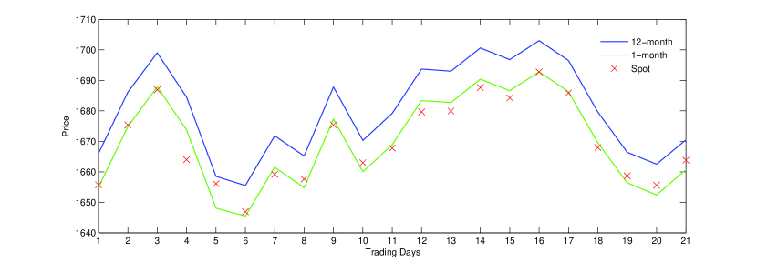
Figure 1: Time evolution of spot gold price, 1-month futures price (Jan-13 contract) and 12 month futures price (Dec-13 contract) over the period from Dec 29, 2012 to Jan 29, 2013. We can see the two futures prices move in parallel, and that the spot price trades very close to the front month futures price.

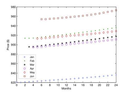
(a) Jan-Jun 2009

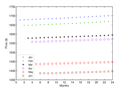
(b) Jan-Jun 2013

Figure 2: Term structures from Jan to Jun in 2009 (left) and 2013 (right).

Next, we compare the linear relationships for returns computed over 5, 10, and 15 trading days. Since we use disjoint time windows for return calculations, a longer holding period implies fewer data points for the regression. In Figure 3, we plot the regressions of 12-month futures returns versus gold returns for both 1-day returns and 10-day returns, plotted on the same $x$-$y$ axis scale. We can see the returns vary on a larger range for the 10-day returns. Spot gold has a 1-day return between -9.07% (4/15/2014) and 4.99% (1/23/2009), while its 10-day returns vary between -9.12% (6/6/2013 to 6/19/2013) and 11.30% (8/5/2011 to 8/18/2011). On the other hand, the 12-month futures has a 1-day return between -9.40% (4/15/2014) and 7.68% (3/19/2009), while its 10-day returns vary between -9.16% (6/6/2013 to 6/19/2013) and 11.30% (8/5/2011 to 8/18/2011). Moreover, we can see that the slope is slightly higher for the 10-day returns versus the 1-day returns.

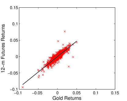
(a) 1-Day Returns

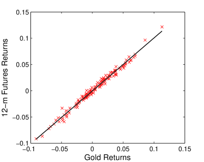
(b) 10-Day Returns

Figure 3: Linear regressions of 12-month futures returns based on 1-day returns (left) and 10-day returns (right) versus the spot gold returns.

This is confirmed numerically and in general for the various futures contracts in Table 3. Here, we give the slopes for the regression of each futures return versus the gold return, while varying the holding period. We display the slopes and $R^{2}$ values from Table 2 for comparison. However, we do not give the intercepts for these regressions as they are all very trivial and effectively 0. We can see that the slopes approach the value 1 as the holding period is lengthened. Thus, the longer the holding period, the more closely the gold return and futures price return are to one another. In particular, the slopes for 10-day returns are all greater than 1, indicating an increased price sensitivity. Furthermore, the strength of this linear relationship increases as can be seen by the increasing $R^{2}$ values in Table 3.

	Days	1-Month	2-Month	6-Month	12-Month
Slope	1	0.94314	0.94301	0.94348	0.94358
	5	0.99805	0.99752	0.99757	0.99715
	10	1.01075	1.01020	1.00970	1.00841
	15	0.99448	0.99461	0.99431	0.99345
$R^{2}$	1	0.80947	0.80911	0.80934	0.80984
	5	0.97154	0.97158	0.97194	0.97165
	10	0.98516	0.98530	0.98572	0.98550
	15	0.98704	0.98691	0.98725	0.98713

Table 3: A summary of the slopes and $R^{2}$ from the regressions of futures returns versus gold returns over different holding periods.

2.2 Static Replication of Gold Spot Price

In this section we consider replication of the gold spot price with a static portfolio of futures contracts. We use portfolios of either 1 or 2 futures contracts and an investment in the money market account. We seek a static portfolio that minimizes the sum of squared errors:

$$SSE=\sum_{j=1}^{n}(V_{j}-G_{j})^{2}\,,$$ (1)

where $V_{j}$ is the dollar value of the portfolio on trading day $j$, while $G_{j}$ is the dollar value of the gold spot price on trading day $j$.

Let $k$ be the number of futures contracts and $\textbf{w}:=(w_{0},\ldots,w_{k})$ be the real-valued vector of portfolio weights. In particular, $w_{0}$ represents the weight given to the money market account. To calculate the optimal portfolio value we will choose weights historically which minimize SSE over the 5-year period 12/22/2008 through 12/22/2013. Thus, we solve the following constrained least squares optimization problem:

$$\underset{\textbf{w}\in{\mathbb{R}}^{k+1}}{\text{min}} \|\textbf{C}\textbf{w}-\textbf{d}\|^{2}$$ (2)

s.t. $$\sum_{j=0}^{k}w_{j}=1$$

The matrix C contains as columns, the historical prices of the various futures contracts and the money market account, and the vector, d contains the historical prices of spot gold. These prices are normalized by $\$1000$, without loss of generality, so that an investor starting with $\$1000$ will invest $$1000\cdot w_{j}$ into the $j$th futures contract and $ $1000\cdot w_{0}$ into the money market account.

We will compare our portfolios to investments in the ETF GLD, which tracks the gold spot price. To do this, we will perform an out-of-sample analysis and compare the values of $\$1000$ invested in GLD and $\$1000$ invested in our constructed portfolio over the period from 12/23/2013 to 7/14/2014. To measure the performance we will use the following root mean squared error for both in-sample and out-of-sample prices:

$$RMSE=\sqrt{\frac{1}{n}\sum_{j=1}^{n}\left({V_{j}-G_{j}}\right)^{2}}\,.$$ (3)

We solve this optimization problem for ten different portfolios with 1 or 2 futures, along with the money market account. The optimal weights, and corresponding in-sample/out-of-sample RMSEs are given in Table 4. In general, the money market account is used minimally as the weights on the account are less than 7% in absolute value for all ten portfolios.

For all the portfolios with 2 futures contracts, the optimal strategy is to go long the shorter term futures contract and short the longer term futures contract, with different weights. The sum of the two resulting weights are approximately 1. In terms of RMSE, the 1-month futures contract appears to be the best replicating instrument of the gold spot. When it is used alone, it performs best relative to other single futures portfolios. When it is used in a pair with another futures, it performs better than any other single futures contract, and better than all other futures pairs: (2-m, 6-m), (2-m, 12-m), and (6-m, 12-m).

	Futures	$w_{0}$	$w_{1}$	$w_{2}$	$RMSE$ (in)	$RMSE$ (out)
1 Futures	1-m	-0.01071	1.01071	-	6.62989	3.34047
	2-m	-0.04835	1.04835	-	12.22148	6.12074
	6-m	-0.05030	1.05030	-	13.23663	5.33971
	12-m	-0.06842	1.06842	-	15.11103	5.71318
2 Futures	1-m, 2-m	-0.00088	1.27315	-0.27227	6.26711	2.79411
	1-m, 6-m	-0.00171	1.23899	-0.23729	6.27232	2.97602
	1-m, 12-m	-0.00021	1.19336	-0.19315	6.28735	3.00006
	2-m, 6-m	-0.04079	5.06602	-4.02523	10.27413	9.37292
	2-m, 12-m	-0.01179	2.94860	-1.93681	9.65705	7.08414
	6-m, 12-m	0.01481	4.80979	-3.82460	9.57938	4.52846

Table 4: A summary of the weights and in/out of sample RMSEs for portfolios of 1 and 2 futures contracts. For portfolios with 2 futures, the weight on the shorter term futures is $w_{1}$. For portfolios with a single futures, we have $w_{2}=0$. The weight assigned to the money market account is denoted by $w_{0}$.

In the sample, the RMSE values for the futures portfolios range from 6.63 to 15.11. Since these values are based on a $\$1000$ investment, this means the error within the sample is between 0.663% and 1.511%, which is quite low. By comparison, our calculations give a RMSE of 2.091% for the gold ETF (GLD) during 12/22/2008 to 12/22/2013. Over this longer horizon of 5 years, our portfolios track the benchmark better than GLD. However, over the more recent, shorter out-of-sample period, 12/23/2013 to 7/14/2014, GLD appears to track spot gold slightly better. The RMSE value for GLD during this period is 0.128%, whereas our best portfolio gives a RMSE of 0.279%. In Figure 4, we show the time series of the optimal static portfolio with the front month futures (top), and the time series for GLD. It is visible that both track the gold spot price closely over this out-of-sample period.

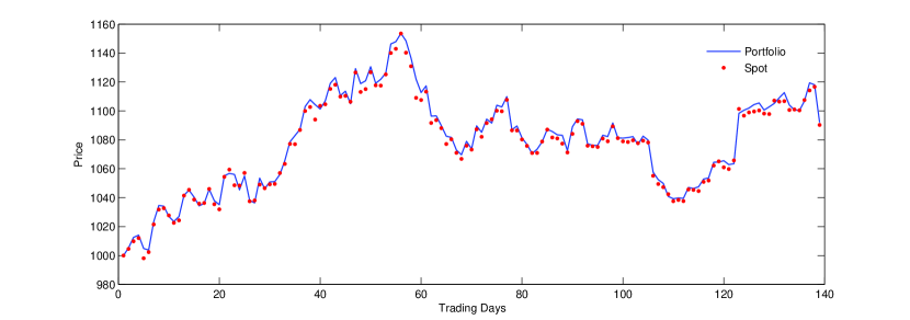
(a) Portfolio with 1-m Futures

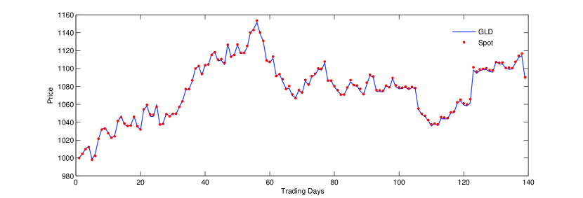
(b) GLD

Figure 4: Out-of-sample time series of our optimal portfolio of front month futures and money market account (top) compared to the spot price, and GLD compared to the spot price (bottom). The trading days are over the period 12/23/2013 to 7/14/2014.

3 Leveraged ETFs

In this section we analyze the returns and tracking performances of various leveraged ETFs. From historical prices of each LETF, we conduct an estimation of the leverage ratio, and investigate the potential deviation from the target leverage ratio. Moreover, we construct a number of static portfolios with futures contracts to seek replication of some leveraged benchmarks. However, the static portfolios fail to effectively track the leveraged benchmarks. This motivates us to consider a dynamic portfolio with futures, which turns out to have a much better tracking performance.

By design, an LETF seeks to provide a constant multiple of the daily returns of an underlying index or asset. Let us denote $\beta\in\{-3,-2,+2,+3\}$ the leverage ratio stated by the LETF, and $R_{j}$ the daily return of the underlying (gold spot). Ideally, the LETF value on day $n$, denoted by $L_{n}$, is given by

$$L_{n}=L_{0}\cdot\prod_{j=1}^{n}(1+\beta\,R_{j}).$$ (4)

We call this the leveraged benchmark, and examine the empirical performance of various LETFs with respect to this benchmark.

For many investors, one appeal of LETFs is that leverage can amplify returns when the underlying is moving in the desired direction. Mathematically, we can see this as follows. Rearranging (4) and taking the derivative of the logarithm, we have

$$\frac{d}{d\beta}\left(\log\left(\frac{L_{n}}{L_{0}}\right)\right)=\sum_{j=1}^{n}\frac{R_{j}}{1+\beta\,R_{j}}.$$ (5)

With a positive leverage ratio $\beta>0$, if $R_{j}>0$ for all $j$, then $\log\left(\frac{L_{n}}{L_{0}}\right)$, or equivalently the value $L_{n}$, is increasing in $\beta$. In other words, when the underlying asset is increasing in value, a larger, positive leverage ratio is preferred. On the other hand, if $R_{j}<0$ for all $j$, and $\beta<0$, a more negative $\beta$ increases $\log\left(\frac{L_{n}}{L_{0}}\right)$ and thus $L_{n}$. This means that when the underlying asset is decreasing in value, a more negative leverage ratio yields a higher return.

The example below illustrates the consequences of maintaining a constant leverage in an environment with non-directional movements:

Day	ETF	%-change	+2x LETF	%-change	$-2$x LETF	%-change
0	100		100		100
1	98	-2%	96	-4%	104	4%
2	99.96	2%	99.84	4%	99.84	-4%
3	97.96	-2%	95.85	-4%	103.83	4%
4	99.92	2%	99.68	4%	99.68	-4%
5	97.92	-2%	95.69	-4%	103.67	4%
6	99.88	2%	99.52	4%	99.52	-4%

Even though the ETF records a tiny loss of 0.12% after 6 days, the +2x LETF ends up with a loss of 0.48%, which is greater (in absolute value) than 2 times the return ($-0.12\%$) of the ETF. We can see this to be the case on any day (e.g. not just the terminal date) except for day 1. For example, on day 3, the ETF has a net loss of 2.04% and the LETF has a net loss of 4.15%, which is greater (in absolute value) than 4.08% (twice the absolute value of the return of the ETF). Furthermore, it might be intuitive that that the $-2$x LETF should have a positive return when the ETF and LETF have negative returns, this is not true. At the terminal date, both the long and short LETFs have recorded net losses of 0.48%. Again, this occurs throughout the period as well, not just the terminal date. In addition to day 6, both the long and short LETFs as well as the ETF itself are in the black. These results are consequences of volatility decay.

Although long and short LETFs are expected to move in opposite directions daily by design, it is often possible for both LETFs to have negative cumulative returns when held over a longer horizon. Figure 5 shows the historical cumulative returns of the gold LETFs UGL (+2x) and GLL ($-2$x) from July 2013 to July 2014. From trading day 124 (1/24/2014) onward, GLL has a negative cumulative return. There are points after trading date 124 where UGL also has a negative cumulative return. In fact, it starts in the black on this date and continues to have a net loss until trading date 146 (2/12/2014). This occurs again a few times, another long stretch where both have a net loss is trading date 210 (5/15/2014) through 233 (6/18/2014).This observation, though maybe counter-intuitive at first glance, is a consequence of daily replication of leveraged returns. The value erosion tends to accelerate during periods of non-directional movements.

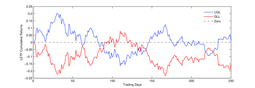
Figure 5: UGL (+2x) and GLL ($-2$x) cumulative returns from July 2013 to July 2014. Observe that both UGL and GLL can give negative returns (below the dotted line of 0%) simultaneously over several periods in time.

3.1 Empirical Leverage Estimation

We conduct a regression analysis and the results are given in Table 5. Each slope is approximately equal to the LETF’s target leverage ratio. In principle, if each (L)ETF is able to generate the desired multiple of daily returns, the slopes of the regression should be equal to the various leverage ratios. In this table, we give an additional two columns for the t-statistic and p-value for testing the hypothesis: $\{H_{0}:\,\text{slope}=\beta\}$ vs. $\{H_{1}:\,\text{slope}\neq\beta\}$. Here, $\beta$ is the target leverage ratio. We can see that each p-value is larger than 0.05 and therefore conclude that statistically, each (L)ETF does not differ from its target leverage ratio. This demonstrates to us that the (L)ETFs are performing exactly as desired, at least on a daily basis.

(L)ETF	Slope	Intercept	t-stat	p-value	$R^{2}$	$RMSE$
GLD	1.00540	$-1.64276\cdot 10^{-5}$	1.42692	0.15382	0.98060	0.00163
UGL	2.00572	$-1.31073\cdot 10^{-4}$	0.73319	0.46357	0.97930	0.00337
GLL	-2.00556	$-1.05504\cdot 10^{-4}$	0.67089	0.50240	0.97673	0.00358
UGLD	2.99358	$-1.98605\cdot 10^{-4}$	0.45211	0.65133	0.98484	0.00421
DGLD	-2.97528	$-1.69127\cdot 10^{-5}$	0.97442	0.33019	0.95256	0.00752

Table 5: A summary of the regression coefficients and measures of goodness of fit for regressing one-day returns of (L)ETFs versus spot gold. We include 2 additional columns for the t-statistic and p-value for testing the hypothesis that the slope equals the leverage ratio in each case.

We see also that the $R^{2}$ values for each regression are quite high, all above 95%. Next, we compare the long and short LETFs for a fixed $|\beta|\in\{2,3\}$. The short LETF tends to have a higher RMSE and lower $R^{2}$ value. Finally, we see in general that as the leverage ratio increases in absolute value, there is a higher RMSE. One possible explanation is that the benchmark is leveraged, and this could magnify the tracking error.

Just as in Section 2.1, we analyze the effects of changing the holding period. In Table 6 we give the slopes and intercepts for the regressions of each (L)ETF’s return versus the spot return while varying the holding period between 1 and 5 days. Our computations show the $R^{2}$ values are all above 95%. We can see that the slopes all approximately equal the target leverage ratio of the (L)ETF. However we notice that in general the intercepts get more negative as the holding period is lengthened. Although they are still quite small, they become more significant as the holding period increases. Our calculations show that the p-values for testing the hypothesis: $\{H_{0}:\,\text{intercept}=0\}$ vs. $\{H_{1}:\,\text{intercept}\neq 0\}$ generally tend to decrease for each (L)ETF. In fact, for UGL the intercepts turn out to be statistically different from 0 (at the 5% level) for holding periods of 3, 4 and 5 days with p-values of 1.37%, 0.57% and 0.33%, respectively. This is consistent with the volatility decay discussed above. We saw there an example where over shorter periods, the LETF tracks its leverage ratio well, but over a longer period it tends to lose money when there is high volatility. The intercepts being different from 0 is akin to the volatility decay in the following sense. Over longer periods, the regressions show that we require more information than just the gold return to predict the LETF return.

To compare the performance of the LETF versus the target multiple of the spot return, we also report in Table 6, the average return differential, defined by

$$\overline{RD}=\frac{1}{m}\sum_{j=1}^{m}\left(R^{(L)}_{j}-\beta\cdot R^{(G)}_{j}\right),$$ (6)

where $m$ is the number of the periods, $R^{(L)}_{j}$ is the LETF’s return over the holding period and $R^{(G)}_{j}$ is the spot’s return over the holding period. We find this to be increasing (in absolute value) with the holding period length. That is, as we hold the LETF longer, it tends to increasingly underperform with respect to the multiple of the underlying return, on average. This is exactly the same notion described above, since over time, the volatility of the underlying causes the LETF to erode in value.

	Days	UGL	GLL	UGLD	DGLD	GLD
Slope	1	2.00572	-2.00556	2.99160	-2.96362	1.00540
	2	2.00828	-2.00395	2.92015	-3.02429	1.00477
	3	1.97770	-1.99661	2.94520	-3.06690	0.99194
	4	2.00071	-2.00908	2.97854	-3.04311	1.00206
	5	2.02081	-2.03273	2.89478	-3.07267	1.01039
Intercept $(\cdot 10^{-4})$	1	-1.31074	-1.05505	-1.98605	-0.16913	-0.16428
	2	-2.73282	-2.28807	-4.23120	-1.81545	-0.33388
	3	-4.06417	-3.96629	-4.97993	-1.05631	-0.40843
	4	-5.44427	-4.62166	-8.08478	-2.69971	-0.66133
	5	-6.81614	-4.82805	-8.03417	-0.30766	-0.92359
$\overline{RD}\,(\cdot 10^{-3})$	1	-0.12892	-0.10760	-0.19673	-0.02414	-0.01439
	2	-0.26677	-0.23191	-0.43999	-0.19081	-0.02964
	3	-0.43253	-0.39265	-0.53511	-0.08462	-0.05028
	4	-0.54331	-0.47645	-0.81687	-0.27854	-0.06290
	5	-0.64076	-0.54705	-0.79183	0.07165	-0.07195

Table 6: A summary of the slopes and intercepts from the regressions of LETF returns versus gold returns, as well as the average return differential ($\overline{RD}$) over different holding periods.

3.2 Static Leverage Replication

In this section, we perform the same optimization as in Section 2.2. We once again seek a static portfolio of futures which minimizes SSE. Let $k$ be the number of futures contracts and $\textbf{w}:=(w_{0},\ldots,w_{k})$ be the real-valued vector of portfolio weights. As before, $w_{0}$ represents the weight given to the money market account. We seek the weights which minimize SSE over the 5-year period 12/22/2008 through 12/22/2013. Thus, we are led to the same constrained least squares optimization problem:

$$\underset{\textbf{w}\in{\mathbb{R}}^{k+1}}{\text{min}} \|\textbf{C}\textbf{w}-\textbf{L}\|^{2}$$ (7)

s.t. $$\sum_{j=0}^{k}w_{j}=1$$

Again, the matrix C contains as columns, the historical prices of the various futures contracts and the money market account. Here, the vector L contains the historical prices of the leveraged benchmark in (4). Without loss of generality, we normalize the prices by $\$1000$ so that our solution will give us a set of weights on each instrument.

We will compare the tracking error of our optimal portfolios to that of investments in the LETFs. To be able to analyze the portfolios we get by solving the optimization problem, we will perform an out of sample analysis over the period 12/23/2013 through 7/14/2014 and see how $\$1000$ invested in the LETFs and $\$1000$ invested in our optimal portfolios perform. To quantify the performance we use the same root mean square error

$$RMSE=\sqrt{\frac{1}{n}\sum_{j=1}^{n}\left({V_{j}-L_{j}}\right)^{2}},$$ (8)

where, $V_{j}$ is the dollar value of the portfolio on trading day $j$, while $L_{j}$ is the dollar value of the leveraged benchmark on trading day $j$. Now, we present the results for the optimization and in sample/out of sample RMSE.

UGL(+2x)	Futures	$w_{0}$	$w_{1}$	$w_{2}$	$RMSE$ (in)	$RMSE$ (out)
1 Futures	1-m	-1.48159	2.48159	-	153.20152	41.48530
	2-m	-1.57601	2.57601	-	140.41254	49.56627
	6-m	-1.58107	2.58107	-	138.63116	47.45953
	12-m	-1.62627	2.62627	-	134.50683	48.29851
2 Futures	1-m, 2-m	-1.94496	-9.89441	12.83937	114.30949	81.36970
	1-m, 6-m	-1.91184	-8.43451	11.34634	113.67580	67.39428
	1-m, 12-m	-2.02222	-6.92791	9.95013	108.29897	67.15776
	2-m, 6-m	-1.64536	-34.26195	36.90731	126.62074	22.64952
	2-m, 12-m	-1.99096	-18.99151	21.98248	111.75046	40.92852
	6-m, 12-m	-2.24344	-35.66917	38.91260	102.86283	62.53830

Table 7: A summary of the weights and in/out of sample RMSEs for portfolios of 1 and 2 futures contracts which attempt to replicate a leveraged benchmark with $\beta=2$. By comparison, the +2x LETF, UGL has an out of sample RMSE of only 5.52485.

GLL($-2$x)	Futures	$w_{0}$	$w_{1}$	$w_{2}$	$RMSE$ (in)	$RMSE$ (out)
1 Futures	1-m	1.97544	-0.97544	-	152.33349	76.14381
	2-m	2.01068	-1.01068	-	155.76147	73.14698
	6-m	2.01234	-1.01234	-	156.43931	74.00595
	12-m	2.02926	-1.02926	-	158.06790	73.79237
2 Futures	1-m, 2-m	1.69510	-8.46293	7.76783	139.27436	100.10091
	1-m, 6-m	1.70510	-7.83463	7.12954	137.98773	92.21120
	1-m, 12-m	1.60773	-7.37540	6.76767	133.31705	93.11206
	2-m, 6-m	1.93900	-39.08635	38.14735	142.57324	43.40713
	2-m, 12-m	1.57681	-23.56157	22.98477	127.90630	62.10415
	6-m, 12-m	1.27887	-43.36906	-43.09020	117.81839	88.35987

Table 8: A summary of the weights and in/out of sample RMSEs for portfolios of 1 and 2 futures contracts which attempt to replicate a leveraged benchmark with $\beta=-2$. By comparison, the $-2$x LETF, GLL has an out of sample RMSE of only 4.76269.

UGLD(+3x)	Futures	$w_{0}$	$w_{1}$	$w_{2}$	$RMSE$ (in)	$RMSE$ (out)
1 Futures	1-m	-3.33704	4.33704	-	555.49151	111.51133
	2-m	-3.50625	4.50625	-	529.90858	125.98635
	6-m	-3.51562	4.51562	-	526.58448	122.33175
	12-m	-3.59587	4.59587	-	518.96896	123.83019
2 Futures	1-m, 2-m	-5.18147	-44.92498	51.10645	379.11676	270.58292
	1-m, 6-m	-5.02680	-38.53507	44.56188	381.92109	213.62168
	1-m, 12-m	-5.41970	-31.91076	38.33046	366.49764	210.91245
	2-m, 6-m	-3.78077	-141.31534	146.09611	472.32904	48.04126
	2-m, 12-m	-5.12561	-79.66101	85.78662	413.19682	98.33728
	6-m, 12-m	-6.14011	-147.04408	154.18419	376.40048	185.87170

Table 9: A summary of the weights and in/out of sample RMSEs for portfolios of 1 and 2 futures contracts which attempt to replicate a leveraged benchmark with $\beta=3$. By comparison, the +3x LETF, UGLD has an out of sample RMSE of only 6.08133.

DGLD($-3$x)	Futures	$w_{0}$	$w_{1}$	$w_{2}$	$RMSE$ (in)	$RMSE$ (out)
1 Futures	1-m	2.14737	-1.14737	-	222.59075	135.67755
	2-m	2.18885	-1.18885	-	225.76707	132.14962
	6-m	2.19079	-1.19079	-	226.42907	133.16229
	12-m	2.21063	-1.21063	-	228.13706	132.91661
2 Futures	1-m, 2-m	1.82654	-9.71612	8.88958	211.09051	163.04734
	1-m, 6-m	1.83531	-9.06486	8.22955	209.75562	154.16271
	1-m, 12-m	1.70781	-8.79773	8.08992	204.41288	155.82542
	2-m, 6-m	2.10262	-46.99103	45.88841	212.78493	95.24835
	2-m, 12-m	1.63980	-29.72604	29.08624	195.74796	117.35419
	6-m, 12-m	1.24461	-55.83130	55.58669	183.42198	150.58261

Table 10: A summary of the weights and in/out of sample RMSEs for portfolios of 1 and 2 futures contracts which attempt to replicate a leveraged benchmark with $\beta=-3$. By comparison, the $-3$x LETF, DGLD has an out of sample RMSE of only 4.43718.

In contrast to the case of tracking the gold spot with futures (see Table 4), the static portfolios do not replicate the leveraged benchmark well here. In Tables 7 through 10, the RMSE values are quite large for all the portfolios. The minimum RMSE for any portfolio of futures trying to replicate any leveraged benchmark is 22.64952 (achieved by a portfolio of 2-month and 6-month futures attempting to replicate a +2x investment in gold) and by comparison the maximum RMSE for any LETF trying to replicate its respective leveraged investment is 6.08133. (This is achieved by UGLD, which tracks a +3x investment in gold.) Unlike the unleveraged investment, the money market account is extensively used throughout the various portfolios. This is interesting but also logical. Indeed, in order to create leverage, the portfolio must either borrow if $\beta>0$ or invest in the money market account if $\beta<0$.

Furthermore, the optimal weights tend to lead to over/underleveraging. Since we are considering an investment in gold, the sum of the weights on the futures (which are proxy’s for investment in gold) can be interpreted as the leverage on the portfolio. Since all the weights sum to 1, we can compute the approximate leverage as $1-w_{0}$. For the +2x and +3x investments, these values are all larger than 2 and 3, respectively. For the $-2$x and $-3$x investments, these values are all smaller (in absolute value) than $-2$ and $-3$, respectively. Granted, these are different instruments than the spot, but we have seen in Section 2.1 they all move in parallel to the spot. Thus we see that the long portfolios tend to be over leveraged, while the short portfolios tend to be under leveraged.

The optimization procedure has led to some rather uneven portfolio weights. For example, the optimal portfolio of 6-month and 12-month futures that attempts to replicate a +3x investment in spot gold requires the following transactions at inception: borrow $6,140.11 from the money market account, short $147,044.08 in 6-month futures and long $154,184.19 in 12-month futures. In practice this would not be possible in the marketplace due to position limits that may be in place.

3.3 Dynamic Leverage Replication

To improve upon the replication in Section 3.2, we now consider a dynamic portfolio of one futures contract. Let $P_{t}$ be our portfolio value at time $t$. At every point in time, the portfolio invests $\beta$ times the value of the fund in the futures contract in order to achieve the required leverage. To fund this investment, the portfolio must borrow from the money market account. As a result, the value of our portfolio has the following dynamics:

$${dP}_{t}=\beta P_{t}\frac{dF_{t}}{F_{t}}-P_{t}(\beta-1)r_{t}dt.$$ (9)

Here, $F_{t}$ is the value of a gold futures contract at time $t$ with a chosen maturity, e.g. 1 month, and $r_{t}$ is the risk free rate at time $t$.

Remark 1

For our empirical analysis, we need not specify a parametric model for the futures price. Nevertheless, if one models the futures price by the stochastic differential equation

$$\frac{dF_{t}}{F_{t}}=\mu_{t}dt+\sigma_{t}dW_{t},$$

with some stochastic drift $(\mu_{t})_{t\geq 0}$ and volatility $(\sigma_{t})_{t\geq 0}$, (many well-known models, including the Heston, and exponential Ornstein-Uhlenbeck models, fit within the above framework) then the log-price of the portfolio is given by

$$\log P_{t}=\log P_{0}+\beta\log\frac{F_{t}}{F_{0}}+\frac{\beta-\beta^{2}}{2}\Sigma_{t}+(1-\beta)R_{t},$$ (10)

where $\Sigma_{t}=\int_{0}^{t}\sigma_{s}^{2}ds$ is the realized variance of $F$ accumulated up to time $t$ and $R_{t}=\int_{0}^{t}r_{s}ds$. Therefore, under this general diffusion model, the log-return of the portfolio is proportional to the log-return of the futures by a factor of $\beta$, but also proportional to the variance by a factor of $\frac{\beta-\beta^{2}}{2}$. The latter factor is negative if $\beta\notin(0,1)$, which is true for every LETF considered here.

To implement the leveraged portfolio in (9), we choose the front month futures contract. Recall from Section 2.2 that the front month futures is the most effective in replicating the spot gold price. To calculate our portfolio value on each trading day, we discretize (9) in time, using $\Delta t$ equal to 1 trading day and set $P_{0}$ equal to $1000 as before.

To quantify our portfolio’s replicating ability we will use the same root mean squared error that we used in Section 3.2:

$$RMSE=\sqrt{\frac{1}{n}\sum_{j=1}^{n}\left({P_{j}-L_{j}}\right)^{2}},$$ (11)

where, $L_{j}$ is the value of a leveraged investment in gold and $P_{j}$ is the value of our portfolio, each at trading day $j$. For this dynamic portfolio, there is no sample from which we will need to draw our weights or train our model in any way. Therefore we can look at any conceivable time period and compare how the LETF $(L)$ or leveraged portfolio $(P)$ performs using the metric in (11).

For this tracking metric, we consider the period 1/3/2012 (first trading day of 2012) to 7/14/2014. The results are shown in Table 11. The portfolio RMSEs range between 0.687% and 3.291%, which are smaller than LETF RMSEs which range between 1.87% and 4.338%. Overall, we see that the portfolio RMSEs are lower than the LETF RMSEs. Indeed, we see that our dynamic portfolio is able to track the target leveraged index quite well according to the RMSE values for $\beta\in\{2,-2,3\}$. However the tracking is not as strong for $\beta=-3$. Nonetheless, the value is quite small and not that far off from the LETF RMSE.

In Figure 6, we see the time evolution for both the dynamic portfolio and GLL compared to the $-2$x benchmark. It is visible that the LETF tends to underperform the benchmark and the difference worsens over time. On the other hand, the portfolio tends to stay close to the benchmark over the entire period. Though not reported here, we observe similar patterns for other gold LETFs.

In Table 11, we also give the annual returns for each asset for the years 2011, 2012 and 2013. For UGLD and DGLD we do not have data for the full year of 2011 (its issue date was 10/17/2011) so we do not have annual returns for these LETFs in 2011. The dynamic portfolio returns range between -69.22% and 107.54% while the LETF returns range between -69.90% and 106.16%. Comparing each year and leverage ratio pair, we find that, except for $\beta=-3$ in 2012, our portfolio outperforms the LETF in each year. Thus, we have shown that in general, a dynamic portfolio consisting of just one futures contract can not only more closely track the target leveraged index, but it also outperforms the respective LETF.

			Annual Returns (%)
$\beta$	Asset	$RMSE$	2011	2012	2013
+2x	UGL	30.33	12.90	2.81	-52.31
	Portfolio	6.87	15.23	6.29	-51.83
$-2$x	GLL	40.12	-29.43	-16.40	67.82
	Portfolio	15.87	-27.06	-14.89	70.57
+3x	UGLD	43.38	-	0.41	-69.90
	Portfolio	12.55	-	5.29	-69.22
$-3$x	DGLD	18.70	-	-23.57	106.16
	Portfolio	32.91	-	-24.51	107.54

Table 11: A summary of the annual returns (over the periods: 1/3/2011-12/31/2011, 1/3/2012-12/31/2012 and 1/2/2013-12/31/2013) and RMSE for each LETF and a dynamic portfolio of front month futures and cash. RMSE values are calculated over the period 1/3/2012-7/14/2014.

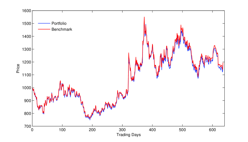
(a) Futures Portfolio

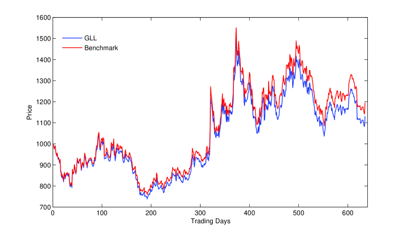
(b) GLL

Figure 6: Time evolution of our dynamic portfolio of front month futures and cash (top) compared to the $-2$x benchmark and GLL (bottom) compared to the $-2$x benchmark. Time period displayed is 1/3/2012 to 7/14/2014.

4 Concluding Remarks

In this paper, we have studied the price relationship among gold spot, futures, ETFs, and leveraged ETFs. There are significant price co-movements among the spot, futures and ETF (GLD). We show that static portfolios consisting 1 or 2 futures with different maturities can effectively replicate the spot gold price. As for leveraged gold ETFs, their average returns tend to be lower than the corresponding multiple ($\beta=3,2,-2,-3$) of the spot’s returns, and the under-performance worsens over a longer holding period. In order to track the leveraged benchmark, we construct a dynamic leveraged portfolio using the 1-month futures. We demonstrate the portfolio tracks the leveraged benchmark better than the corresponding LETFs, and has better returns over multiple years.

As the ETF market continued to grow in quantity and complexity in various asset classes, it is important for both investors and regulators to understand the price dependency among unleveraged and leveraged ETFs, as well as their underlying assets and related derivatives. We have explored futures contracts on gold as a replicating instrument for gold (L)ETFs. It would therefore be important to continue the study of the gold futures market and its impact on the dynamics of LETFs.

As for other future research, there are also options written on gold (L)ETFs. This calls for consistent pricing of LETF options across leverage ratios (see Leung and Sircar (2014)). Also, one can analyze the market impact (see e.g. Dobi and Avellaneda (2012)) of the (L)ETF issuer on the particular derivative market used to replicate the (L)ETF. As we have noted before, (L)ETFs have large market capitalization and thus, an adjustment of the issuer’s portfolio could lead to large movements in the derivatives market used to hedge the (L)ETF. The risks associated with (L)ETFs, futures and other derivatives need to be studied in depth in order to help advise and motivate policies issued by the Fed (see e.g. Chang et al. (2011) for a study of the risk of VIX futures).

Finally, studies that can shed light on the risks of LETFs (see e.g. Leung and Santoli (2012)), and their impact on the broader financial market will be very useful. In the recent study, Skum and Kang (2013) examine the performance of LETFs during the financial crisis. We have seen LETFs on gold have failed to track the desired leveraged target. There are a number of reasons that may contribute to the tracking errors including, but not limited to, illiquidity and risks of the hedging instruments, management fees and financing costs (see e.g. Charupat and Miu (2014)). Studies that illuminate the significance of each of these effects would be useful for investors as well as regulators.

References

- Alexander and Barbosa (2008) Alexander, C. and Barbosa, A. (2008). Hedging index exchange traded funds. Journal of Banking and Finance, 32:326–337.
- Avellaneda and Zhang (2010) Avellaneda, M. and Zhang, S. (2010). Path-dependence of leveraged ETF returns. SIAM Journal of Financial Mathematics, 1:586–603.
- Baur (2012) Baur, D. G. (2012). Asymmetric volatility in the gold market. Journal of Alternative Investments, 14(4):26–38.
- Baur (2013) Baur, D. G. (2013). Exchange-traded funds on gold - a free lunch? Working Paper.
- Baur and Thomas (2010) Baur, D. G. and Thomas, K. (2010). Is gold a safe haven? International evidence. Journal of Banking and Finance, 34(8):1886–2898.
- Chang et al. (2011) Chang, C., Jiménez-Martín, J., McAleer, M., and Pérez-Amaral, T. (2011). Risk management of risk under the Basel Accord: forecasting value-at-risk of VIX futures. Managerial Finance, 37(11):1088–1106.
- Charupat and Miu (2014) Charupat, N. and Miu, P. (2014). A new measure of performance of leveraged exchange-traded funds. The Financial Review, 49(4):735–763.
- Cheng and Madhavan (2009) Cheng, M. and Madhavan, A. (2009). The dynamics of leveraged and inverse exchange-traded funds. Journal of Investment Management, 4.
- Dobi and Avellaneda (2012) Dobi, D. and Avellaneda, M. (2012). Structural slippage of leveraged ETFs. Working Paper.
- Dunis et al. (2013) Dunis, C., Laws, J., Middleton, P., and Karathanasopoulos, A. (2013). Nonlinear forecasting of the gold miner spread: An application of correlation filters. Intelligent Systems in Accounting, Finance and Management, 20(4):207–231.
- Ghosh et al. (2004) Ghosh, D., Levin, E. J., MacMillan, P., and Wright, R. E. (2004). Gold as an inflation hedge? Studies in Economics and Finance, 22(1):1–25.
- Guedj et al. (2011) Guedj, I., Li, G., and McCann, C. (2011). Futures-based commodities ETFs. The Journal of Index Investing, 2(1):14–24.
- Guo and Leung (2014) Guo, K. and Leung, T. (2014). Understanding the tracking errors of commodity leveraged ETFs. In Aid, R., Ludkovski, M., and Sircar, R., editors, Commodities, Energy and Environmental Finance, Fields Institute Communications. Springer.
- Holzhauer et al. (2013) Holzhauer, H., Lu, X., McLeod, R. W., and Mehran, J. (2013). Bad news bears: Effects of expected market volatility on daily tracking error leveraged bull and bear ETFs. Managerial Finance, 39(12):1169–1187.
- Ivanov (2013) Ivanov, S. (2013). The influence of ETFs on the price discovery of gold, silver and oil. Journal of Economics and Finance, 37:453–462.
- Jarrow (2010) Jarrow, R. (2010). Understand the risks of leveraged ETFs. Finance Research Letters, 7(135-139).
- Leung and Li (2014) Leung, T. and Li, X. (2014). Optimal mean reversion trading with transaction costs and stop-loss exit. International Journal of Theoretical and Applied Finance. Forthcoming.
- Leung and Santoli (2012) Leung, T. and Santoli, M. (2012). Leveraged ETFs: Admissible leverage and risk horizon. Journal of Investment Strategies, 2(1):39–61.
- Leung and Sircar (2014) Leung, T. and Sircar, R. (2014). Implied volatility of leveraged ETF options. Applied Mathematical Finance. Forthcoming.
- Murphy and Wright (2010) Murphy, R. and Wright, C. (2010). An empirical investigation of the performance of commodity-based leveraged ETFs. The Journal of Index Investing, 1(3):14–23.
- Naylor et al. (2011) Naylor, M., Wongchoti, U., and Gianotti, C. (2011). Abnormal returns in gold and silver exchange traded funds. The Journal of Index Investing, 2(2):1–34.
- Rompotis (2011) Rompotis, G. (2011). Predictable patterns in ETFs’ return and tracking error. Studies in Economics and Finance, 28(1):476–508.
- Skum and Kang (2013) Skum, P. and Kang, J. (2013). Leveraged and inverse ETF performance during the financial crisis. Managerial Finance, 39(5):476–508.
- Smales (2015) Smales, L. A. (2015). Asymmetric volatility response to news sentiment in gold futures. Journal of International Financial Markets, Institutions and Money, 34:161–172.
- Triantafyllopoulos and Montana (2011) Triantafyllopoulos, K. and Montana, G. (2011). Dynamic modeling of mean-reverting spreads for statistical arbitrage. Computational Management Science, 8(1-2):23–49.