CHAOS I. Direct Chemical Abundances for H II Regions in NGC 628

Abstract

The CHemical Abundances of Spirals (CHAOS) project leverages the combined power of the Large Binocular Telescope (LBT) with the broad spectral range and sensitivity of the Multi Object Double Spectrograph (MODS) to measure “direct” abundances (based on observations of the temperature-sensitive auroral lines) in large samples of H II regions in spiral galaxies. We present LBT MODS observations of 62 H II regions in the nearby spiral galaxy NGC 628, with an unprecedentedly large number of auroral lines measurements (18 [O III] $\lambda 4363$, 29 [N II] $\lambda 5755$, 40 [S III]$\lambda 6312$, and 40 [O II] $\lambda\lambda 7320,7330$ detections) in 45 H II regions. Comparing derived temperatures from multiple auroral line measurements, we find: (1) a strong correlation between temperatures based on [S III] $\lambda 6312$ and [N II] $\lambda 5755$; and (2) large discrepancies for some temperatures based on [O II] $\lambda\lambda 7320,7330$ and [O III] $\lambda 4363$. Both of these trends are consistent with other observations in the literature, yet, given the widespread use and acceptance of [O III] $\lambda 4363$ as a temperature determinant, the magnitude of the T[O III] discrepancies still came as a surprise. Based on these results, we conduct a uniform abundance analysis prioritizing the temperatures derived from [S III] $\lambda 6312$ and [N II] $\lambda 5755$, and report the gas-phase abundance gradients for NGC 628. Relative abundances of S/O, Ne/O, and Ar/O are constant across the galaxy, consistent with no systematic change in the upper IMF over the sampled range in metallicity. These alpha-element ratios, along with N/O, all show small dispersions ($\sigma\sim 0.1$ dex) over 70% of the azimuthally averaged radius. We interpret these results as an indication that, at a given radius, the interstellar medium in NGC 628 is chemically well-mixed. Unlike the gradients in the nearly temperature-independent relative abundances, O/H abundances have a larger intrinsic dispersion of $\sim$ 0.165 dex. We posit that this dispersion represents an upper limit to the true dispersion in O/H at a given radius and that some of that dispersion is due to systematic uncertainties arising from temperature measurements.

1. INTRODUCTION

The chemical evolution of galaxies, whereby successive generations of stars enrich the interstellar medium (ISM) with products from stellar nucleosynthesis, is key to gaining a deeper understanding of galaxy evolution. H II regions can be used to study the absolute and relative abundances in the ISM of spiral galaxies. Thus, spiral galaxies in the nearby universe, with low inclinations, provide the opportunity for studying and understanding the chemical evolution of galaxies.

Chemical abundances have been widely studied in spiral galaxies using “strong-line” calibrations, where ratios of the strong forbidden lines are used as abundance indicators. However, these measurements are only statistical indications of chemical abundance, and are limited by the parameter space of the calibration sample (e.g., van Zee & Haynes, 2006; Bresolin, 2007; Yin et al., 2007; Bresolin et al., 2009a; Stasińska, 2010; Amorín et al., 2010; Berg et al., 2011). Because spiral galaxies exhibit abundance gradients and large ranges in temperature, density, and excitation space (among other parameters), “strong-line” calibrations are vulnerable to large systematic uncertainties (Kewley & Ellison, 2008; Moustakas et al., 2010). In contrast, the “direct” method uses the temperature-sensitive ratio of auroral to forbidden emission lines in order to determine the electron temperature and subsequent chemical abundances.

Due to the inherent challenges of the direct method, detailed direct abundance studies exist for only a handful of spiral galaxies (e.g., 20 H II regions with direct abundances in M101, Kennicutt et al. (2003b); 61 H II regions with direct abundance in M33, Rosolowsky & Simon (2008)). This relative dearth of large samples of direct abundances in the ISM of spiral galaxies prevents us from understanding key processes in the evolution of galaxies and limits our ability to fully understand: the chemical abundance gradients in spirals; the dispersion in the ISM abundances as a function of radius and environment; the yields of elements from stellar nucleosynthesis with potential constraints on the stellar initial mass function; the chemical evolution of galaxies at high redshift; and thus, the chemical enrichment history of the universe. In order to place these measurements on the same scale for comparison amongst galaxies, reliable and consistent derivations of abundances are needed (see, e.g., Moustakas et al., 2010).

With recognition that simply measuring a direct abundance is not the panacea to all H II region abundance measurement problems, assembling large, homogeneous datasets of electron temperature measurements represent our best observational approach to putting all H II region abundance measurements on firmer ground. Increasing the number of H II regions observed per galaxy allows for statistical approaches to questions about discrepant electron temperature measurements (e.g., Kennicutt et al., 2003b; Binette et al., 2012), dispersions in abundances at a given radius (e.g., Kennicutt et al., 2003b; Rosolowsky & Simon, 2008), and dispersions as a function of environment (e.g., Kennicutt et al., 2003b).

1.1. The CHAOS Project

The CHemical Abundances Of Spirals (CHAOS) project was undertaken in order to build a large database of high quality H II region spectra from nearby spiral galaxies using the Multi-Object Double Spectrographs (MODS; Pogge et al., 2010) on the Large Binocular Telescope (LBT). The MODS have been designed to optimally obtain high quality spectra across fields of view (6′$\times$6′) comparable to the extents of nearby spiral galaxies. Furthermore, the LBT and MODS combination provides the balance between sensitivity, resolution, and wavelength coverage necessary to measure all emission lines relevant to oxygen, nitrogen, and alpha-element abundance determinations and more. In particular, the optical design of MODS has been optimized for high throughput in the red and blue channels to produce high-quality spectrophotometry from the atmospheric UV cut-off ($\sim$340 nm) to the silicon detector cutoff at $\sim$1$\mu$m.

The Spitzer Infrared Nearby Galaxies Survey (SINGS; Kennicutt et al., 2003a) galaxies are arguably the best understood spiral galaxies outside of the Local Group due to having the most complete multi-wavelength observations available. Due to the Spitzer observations and large ancillary data sets, these galaxies have resolved 3.6-160 $\mu$m imaging, 5-40 $\mu$m IRS spectroscopy of the central regions plus select extra-nuclear H II regions, and high-quality H I and CO gas maps with detailed 2-D rotation curves. Additionally, observations by Herschel under the Key Insights on Nearby Galaxies: a Far- Infrared Survey with Herschel project (KINGFISH; Kennicutt et al., 2011) provide PACS and SPIRE imaging, as well as far-IR spectroscopy of selected H II regions. We defined the CHAOS sample by identifying the optimal candidates within the SINGS sample: we restrict our sample to nearly face-on, luminous (M${}_{B}<-18$ mag), spiral galaxies (Hubble type T $>0$) accessible from the northern hemisphere with the LBT (declination $>-5^{\circ}$), with minimal transit airmasses ($<1.1$). For our final target sample, 13 high priority SINGS galaxies were selected.

The collection of a large sample of H II regions is driven by the need to precisely measure the form of the radial gradient, including deviations from simple linear fits, and the dispersion in abundance at fixed radius. Ideally, roughly 10 H II regions in approximately 10 independent radial bins, or $\sim$ 100 H II regions per galaxy, would be required to achieve the desired precision. Given the steep H II region luminosity function, and the non-random distribution of H II regions in a spiral galaxy, this ideal statistical sample is not obtainable for all galaxies, but represents a reasonable goal. At present, multiple fields have been observed in 9 of the 13 galaxies, already more than doubling the number of H II regions in spiral galaxies with sufficient quality spectra to provide accurate measurements of the physical conditions (i.e., temperatures, densities, and ionization parameters) and absolute and relative chemical abundances.

1.2. NGC 628 Properties

We present LBT observations of H II regions in the first CHAOS target, NGC 628. NGC 628 (M 74) is a late-type giant Sc spiral galaxy with a systematic velocity of 656 km s^-1. We adopt a distance of 7.2 Mpc (Van Dyk et al., 2006) and an inclination of $i\approx 5^{\circ}$ (Shostak & van der Kruit, 1984), with a resulting scale of 35 pc arcsec^-1. The adopted properties for NGC 628 are provided in Table 1. NGC 628 is an excellent target due to its small inclination, extended structure, and undisturbed optical profile. The gas-phase oxygen abundance of NGC 628 has been studied previously using long-slit or fiber spectroscopy (Talent, 1983; McCall et al., 1985; Zaritsky et al., 1994; Ferguson et al., 1998; van Zee et al., 1998b; Bresolin et al., 1999; Castellanos et al., 2002; Moustakas et al., 2010; Gusev et al., 2012; Cedrés et al., 2012; Berg et al., 2013), and integral field spectroscopy (Rosales-Ortega et al., 2011; Croxall et al., 2013). All together, a combined total of 18 distinct H II region direct abundance measurements exist in the literature for NGC 628 (Castellanos et al., 2002; Berg et al., 2013; Croxall et al., 2013). The CHAOS observations of NGC 628 present a three-fold increase in the total number of direct H II region abundances and allow, for the first time, the spatial variations and dispersions in absolute and relative ISM abundances to be determined from the direct method.

This paper is organized as follows: In Section 2 we describe the LBT observations for NGC 628, the spectral data processing, the emission line measurements, and the reddening corrections. In Section 3 we discuss the derivation of the temperatures and densities of the H II regions, including the choice of atomic data and comparison of the derived temperatures. Our derived abundances are presented in Section 4, where we introduce our uniform abundance analysis method and report ionic and absolute abundances for NGC 628. We further interpret the CHAOS abundance gradients for NGC 628 by considering electron temperature discrepancies (§ 5.1), comparing to the abundance gradients in the literature (§ 5.2), and assessing the physical basis for dispersions at a given galactocentric radius. Finally, we summarize our findings in Section 6. We also present additional analyses in two Appendices: The direct oxygen abundance gradient based on [O III] $\lambda 4363$ electron temperature measurements is presented in Appendix A. Indicators of temperature discrepancies are presented in Appendix B.

Table 1Properties of NGC 628

Property	NGC 628
R.A.	01:36:41.747
Dec.	15:47:01.18
Type	ScI
Adopted D (Mpc)	7.2$\pm$1.01
$m_{B}$ (mag)	9.952
Redshift	0.002192
Inclination (degrees)	53
P.A. (degrees)	124
$R_{25}$ (arcmin)	5.255
$R_{25}$ (kpc)	10.95

Note. — Adopted properties for NGC 628. Rows 1 and 2 give the RA and Dec of the optical center in units of hours, minutes, and seconds, and decrees, arcminutes, and arcseconds respectively. Row 5 lists redshifts taken from the NASA/IPAC Extragalactic Database. Row 8 gives the optical radius at the $B_{25}$ mag arcsec^-2 of the system. Row 9 gives the optical radius of the galaxy given the adopted distance. References: (1) Van Dyk et al. (2006); (2) Lee et al. (2011); (3) Shostak & van der Kruit (1984); (4) Egusa et al. (2009); (5) Kendall et al. (2011)

2. CHAOS SPECTROSCOPIC OBSERVATIONS

2.1. Observation Plan

Optical spectra of NGC 628 were acquired with MODS1 on the LBT as part of the CHAOS project on the UT dates of 2012 October 14 and 16. The primary goal was to obtain high signal-to-noise spectra, with detections of intrinsically faint auroral lines (e.g., [O III] $\lambda$4363, [N II] $\lambda$5755, [S II] $\lambda$6312) at a significance of 3$\sigma$ or higher. The multi-object mode of MODS, which uses custom-designed, laser-milled slit masks, allows spectra of many H II regions to be obtained simultaneously. Broad-band and H$\alpha$ continuum-subtracted SINGS images for NGC 628 (Muñoz-Mateos et al., 2009) were used to identify target H II regions, as well as alignment stars, and determine accurate astrometry for the masks. H II regions were selected to achieve large radial coverage of the optical disk, prioritizing knots of highest H$\alpha$ surface brightness. We observed three multi-slit masks, each containing $\sim$20 slits, which spanned the radial and azimuthal extent of the optical disk of NGC 628. All H II region slits are 1.0″ wide, but lengths vary between $8-20$″ depending on the size of the targeted H II region and proximity of other slits on the mask. Blue and red spectra were obtained simultaneously using the G400L (400 lines mm^-1, R$\sim$1850) and G670L (250 lines mm^-1, R$\sim$2300) gratings, respectively. This combination results in a broad spectral coverage extending from 3200 - 10,000 Å, that was linearly re-sampled to 0.5 Å per pixel and full width half maximum resolution of $\sim$ 2 Å.

Each mask field was observed for six 1200 second exposures, for a total integration time of two hours. The masks were designed with slits at a fixed position angle which approximated the parallactic angle at the midpoint of the longest possible observation window in a night. For NGC 628, during the observing run of UTC 2012 October 2$-$17, we selected the parallactic angle of PA $=-235.2^{\circ}$ for Fields 1 and 3, and PA $=-55.1^{\circ}$ for Field 2, which is just a rotation of $180^{\circ}$ to allow for the use of different guide stars and thus a shift of the field center. This, in addition to observing the galaxies at airmasses less than 1.5, served to minimize the wavelength-dependent light loss due to differential atmospheric refraction (Filippenko, 1982). On the nights that NGC 628 was observed, the sky conditions were optimal: clear, low wind, and low humidity. Additionally, we aimed for approximately arcsecond seeing. Fields 1, 2, and 3 had average seeing values over their 2 hour observation windows of 1.1, 1.25, and 0.85 arcseconds, respectively.

Figure 1 shows the H$\alpha$ continuum-subtracted SINGS image for NGC 628 (Muñoz-Mateos et al., 2009), with slit positions from Table 2 shown as colored lines for each mask field. Throughout this work, all target locations (extraction of H II region; not slit center) are referred to by their offsets in right ascension and declination from the center of NGC 628, which is taken to be $01^{h}36^{m}41.7^{s}$ $+15^{\circ}47$′01″. Slit locations and offsets for all observed H II regions are listed in Table 2.

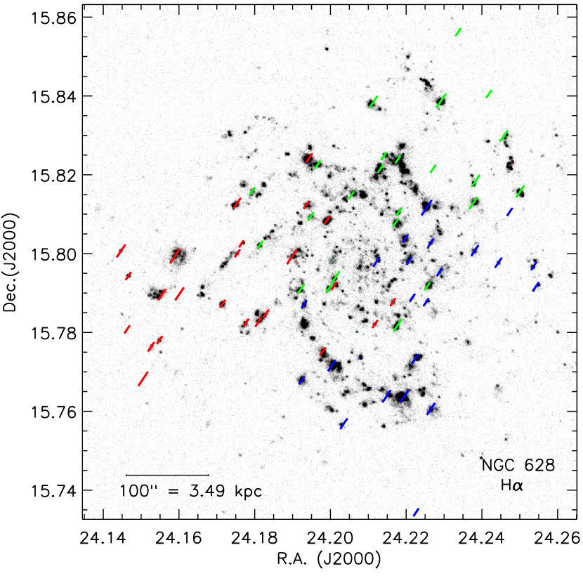
Figure 1.— Continuum-subtracted H$\alpha$ SINGS image of NGC 628 (Muñoz-Mateos et al., 2009). The footprints of CHAOS slits are overlaid, where red, green, and blue respectively represent the Field 1, 2, and 3 slit positions observed at the LBT. The slit positions targeted H II regions, although not always centered in order to maximize effective usage of mask real estate. See Table 2 for more details.

Table 2Logs for NGC 628 LBT Observations

H ii	R.A.	Dec.	Rg	R/R25	Rg	Offset (R.A., Dec.)	Auroral Line Detections
Region	(2000)	(2000)	(arcsec)		(kpc)	(arcsec)	[O iii]	[N ii]	[S iii]	[O ii]	[S ii]
Total Detections:							18	29	40	40	0
NGC628-12.7+2.1	1:36:40.92	15:47:02.06	12.037	0.038	0.42	-12.7,+2.1
NGC628+38.6-17.8	1:36:44.47	15:46:42.19	43.863	0.139	1.53	+38.6,-17.8
NGC628-48.8+0.7	1:36:38.42	15:47:00.72	48.194	0.153	1.68	-48.8,+0.7
NGC628+38.9-26.7	1:36:44.49	15:46:33.32	48.628	0.154	1.69	+38.9,-26.7
NGC628-44.7+27.3	1:36:38.70	15:47:27.34	51.311	0.163	1.79	-44.7,+27.3
NGC628-33.2+45.8	1:36:39.50	15:47:45.80	55.297	0.176	1.93	-33.2,+45.8
NGC628-30.7-46.5	1:36:39.67	15:46:13.48	56.337	0.179	1.97	-30.7,-46.5
NGC628+48.0-32.0	1:36:45.13	15:46:27.98	59.216	0.188	2.07	+48.0,-32.0
NGC628-35.9+57.7	1:36:39.31	15:47:57.72	66.695	0.212	2.33	-35.9,+57.7		✓	✓
NGC628-55.5-40.4	1:36:37.96	15:46:19.64	68.798	0.218	2.40	-55.5,-40.4
NGC628+49.8+48.7	1:36:45.25	15:47:48.72	69.474	0.221	2.43	+49.8,+48.7		✓	✓	✓
NGC628-8.3-72.8	1:36:41.23	15:45:47.18	74.386	0.236	2.59	-8.3,-72.8
NGC628-73.1-27.3	1:36:36.73	15:46:32.68	77.973	0.248	2.72	-73.1,-27.3			✓	✓
NGC628-76.2+22.9	1:36:36.52	15:47:22.91	78.816	0.250	2.75	-76.2,+22.9		✓	✓	✓
NGC628+18.5+79.0	1:36:43.08	15:48:19.02	80.178	0.255	2.80	+18.5,+79.0
NGC628-36.8-73.4	1:36:39.25	15:45:46.65	82.827	0.263	2.89	-36.8,-73.4		✓		✓
NGC628-73.1-44.8	1:36:36.74	15:46:15.18	85.853	0.273	3.00	-73.1,-44.8
NGC628+68.5+53.4	1:36:46.54	15:47:53.35	86.834	0.276	3.04	+68.5,+53.4		✓	✓	✓
NGC628-87.5-10.8	1:36:35.74	15:46:49.16	87.870	0.279	3.07	-87.5,-10.8
NGC628+81.6-32.3	1:36:47.45	15:46:27.69	89.257	0.283	3.11	+81.6,-32.3			✓
NGC628-68.5+61.7	1:36:37.05	15:48:01.74	91.116	0.289	3.18	-68.5,+61.7		✓	✓	✓
NGC628+76.9-49.6	1:36:47.13	15:46:10.42	93.074	0.295	3.25	+76.9,-49.6		✓	✓	✓
NGC628+94.2+4.0	1:36:48.33	15:47:03.99	95.361	0.303	3.33	+94.2,+4.0
NGC628+75.4+66.0	1:36:47.02	15:48:06.01	100.177	0.318	3.50	+75.4,+66.0
NGC628-13.1+107.5	1:36:40.89	15:48:47.50	107.076	0.340	3.73	-13.1,+107.5		✓	✓	✓
NGC628+53.5-104.0	1:36:45.51	15:45:16.04	118.496	0.376	4.13	+53.5,-104.0		✓		✓
NGC628-35.7+119.6	1:36:39.33	15:48:59.59	123.566	0.392	4.31	-35.7,+119.6		✓	✓	✓
NGC628-20.3+124.6	1:36:40.40	15:49:04.62	125.033	0.397	4.36	-20.3,+124.6		✓	✓	✓
NGC628-59.6-111.6	1:36:37.67	15:45:08.43	127.196	0.404	4.44	-59.6,-111.6		✓	✓	✓
NGC628+61.2+113.5	1:36:46.04	15:48:53.45	128.290	0.407	4.48	+61.2,+113.5		✓	✓	✓
NGC628-128.4+13.1	1:36:32.90	15:47:13.09	128.700	0.409	4.50	-128.4,+13.1
NGC628+42.6-120.7	1:36:44.75	15:44:59.30	129.490	0.411	4.52	+42.6,-120.7		✓	✓	✓
NGC628+131.9+18.5	1:36:50.94	15:47:18.53	134.275	0.426	4.69	+131.9,+18.5	✓	✓	✓	✓
NGC628+71.2+121.3	1:36:46.74	15:49:01.32	140.117	0.445	4.90	+71.2,+121.3
NGC628+125.4-62.4	1:36:50.49	15:45:57.61	141.767	0.450	4.95	+125.4,-62.4			✓	✓
NGC628-130.9+71.8	1:36:32.73	15:48:11.80	148.566	0.472	5.18	-130.9,+71.8		✓	✓	✓
NGC628+131.7-70.2	1:36:50.93	15:45:49.80	151.024	0.479	5.27	+131.7,-70.2			✓	✓
NGC628+151.0+22.3	1:36:52.26	15:47:22.33	153.790	0.488	5.37	+151.0,+22.3	✓	✓	✓	✓
NGC628-157.9-0.3	1:36:30.86	15:46:59.71	157.687	0.501	5.51	-157.9,-0.3		✓	✓	✓
NGC628-24.5-155.6	1:36:40.10	15:44:24.39	158.586	0.503	5.54	-24.5,-155.6		✓	✓	✓
NGC628-129.8+94.7	1:36:32.81	15:48:34.73	159.867	0.508	5.58	-129.8,+94.7		✓	✓	✓
NGC628+158.5+9.2	1:36:52.78	15:47:09.20	160.025	0.508	5.58	+158.5,+9.2				✓
NGC628+78.6-137.6	1:36:47.24	15:44:42.37	160.143	0.508	5.59	+78.6,-137.6				✓
NGC628+140.3+82.0	1:36:51.52	15:48:21.99	162.919	0.517	5.68	+140.3,+82.0			✓
NGC628-42.8-158.2	1:36:38.84	15:44:21.79	164.834	0.523	5.75	-42.8,-158.2	✓	✓	✓	✓
NGC628+147.9-71.8	1:36:52.05	15:45:48.18	166.229	0.528	5.80	+147.9,-71.8		✓		✓
NGC628+163.5+64.4	1:36:53.13	15:48:04.34	176.489	0.560	6.16	+163.5,+64.4		✓	✓	✓
NGC628-4.5+185.6	1:36:41.49	15:50:05.63	184.519	0.586	6.44	-4.5,+185.6		✓	✓	✓
NGC628+176.7-50.0	1:36:54.04	15:46:09.96	185.425	0.589	6.47	+176.7,-50.0			✓	✓
NGC628-76.2-171.8	1:36:36.52	15:44:08.22	188.715	0.599	6.59	-76.2,-171.8	✓		✓	✓
NGC628+31.6-191.1	1:36:43.99	15:43:48.85	195.131	0.619	6.81	+31.6,-191.1	✓	✓	✓	✓
NGC628-200.6-4.2	1:36:27.90	15:46:55.81	200.634	0.637	7.00	-200.6,-4.2	✓	✓	✓	✓
NGC628-184.7+83.4	1:36:29.00	15:48:23.36	202.182	0.642	7.06	-184.7,+83.4	✓	✓	✓	✓
NGC628-206.5-25.7	1:36:27.49	15:46:34.31	208.222	0.661	7.27	-206.5,-25.7	✓		✓	✓
NGC628-90.1+190.2	1:36:35.56	15:50:10.17	209.327	0.665	7.31	-90.1,+190.2	✓	✓	✓	✓
NGC628-168.2+150.8	1:36:30.14	15:49:30.77	225.204	0.715	7.86	-168.2,+150.8	✓		✓	✓
NGC628+232.7+6.6	1:36:57.92	15:47:06.58	234.411	0.744	8.19	+232.7,+6.6	✓		✓	✓
NGC628+237.6+3.0	1:36:58.26	15:47:02.93	239.203	0.759	8.35	+237.6,+3.0	✓		✓	✓
NGC628+254.3-42.8	1:36:59.42	15:46:17.11	259.853	0.825	9.07	+254.3,-42.8	✓		✓
NGC628+252.1-92.1	1:36:59.26	15:45:27.85	270.527	0.859	9.45	+252.1,-92.1	✓	✓	✓
NGC628+261.9-99.7	1:36:59.94	15:45:20.24	282.451	0.897	9.89	+261.9,-99.7	✓
NGC628+265.2-102.2	1:37:00.17	15:45:17.76	286.416	0.909	10.00	+265.2,-102.2	✓
NGC628+289.9-17.4	1:37:01.89	15:46:42.55	292.382	0.928	10.20	+289.9,-17.4	✓		✓	✓
NGC628+298.4+12.3	1:37:02.47	15:47:12.26	300.442	0.954	10.49	+298.4,+12.3	✓		✓	✓

Note. — Observing logs for H II regions observed in NGC 628 using MODS of the LBT on the UT dates of 14 and 16 October 2012. Each field was observed over an integrated exposure time of 1200 s on clear nights, with on average $\sim 1\arcsec$ seeing, and airmasses less than 1.5. H II region IDs are listed in Column 1, labeled according to their offsets, and ordered by increasing galactocentric radius. The right ascension and declination of the individual H II regions are given in units of hours, minutes, and seconds, and decrees, arcminutes, and arcseconds respectively. The H II region distances from the center of the galaxy in arcseconds, fraction of $R_{25}$, and in kpc are listed in the Columns 4-6. Additionally, the offsets from galaxy center R.A. and Dec. are given in arcseconds in Column 7. Finally, Columns 8-12 highlight which regions have [O III] $\lambda 4363$, [N II] $\lambda 5755$, [S III] $\lambda 6312$, O II] $\lambda\lambda 7320,7330$, and S II] $\lambda\lambda 4068,4076$ auroral lines detections at the 4$\sigma$ significance level.

2.2. Spectral Reductions

Spectra are reduced and analyzed using the beta-release version of the MODS reduction pipeline. Bias subtraction and flat-fielding were performed using python scripts designed to accommodate the interlaced data read-out. The pixel flat is assembled from slitless lamp flats of the incandescent continuum lamp. Slit definitions, wavelength calibration, and creation of variance images are performed using new tools written to work within the XIDL reduction package. Slit locations on two-dimensional images are defined by mapping laser-milled mask positions and wavelength to pixel coordinates on the CCD. Wavelength calibrations are very stable, modulo a small flexure shift of order a few pixels. Spectra of Hg + Ar, Ne, and Xe + Kr lamps are taken through the slit masks during a calibration sequence performed at the beginning of the observing run. Because the MODS spectrographs are remarkably stable, the optical path is mapped by using the images of lamps through specially designed pinhole masks. With this information, we generate a transformation from an X/Y location on the mask to a pixel on the detector as a function of wavelength, and this geometric transformation allows the construction of an initial trace. The initial spectral traces are corrected for atmospheric refraction using the hour angle and airmass corresponding to the mid-point of the observation. This extraction technique was designed for and is effective for use with very faint spectra where continua are faint or not visible. No slit-losses are observed above 3500 Å  and so no correction is made to this end.

Due to the large angular size of NGC 628, the diffuse ionized medium fills the majority of each field of view. In order to facilitate accurate sky subtraction, additional “sky” slits are placed well away from both H II regions and the main body of the galaxy. Due to the off-axis nature of the sky-slits, they are more affected by aberration than slits targeting H II regions. A sky frame was created by fitting a two-dimensional B-spline to the background sky in the two-dimensional spectra, i.e., each slit is fit independently with a local sky. The continuum flux from the sky-slit is scaled to the background continuum measured locally in each slit. Subsequently, the background under the strong nebular lines is interpolated from the scaled sky-slit to create the final sky-model that is subtracted.

One-dimensional spectra are corrected for atmospheric extinction and flux calibrated based on observations of CALSPEC flux standard stars (Bohlin, 2010). The flux standards are observed on each night science data are obtained. We confirm the high level of fidelity across the spectra by comparing the continuum levels of the red and blue spectra and find that corrections for matching the two sides are on the order of $\sim 1\%$. An example flux-calibrated spectrum is shown in Figure 2.

NGC 628-42.8-158.2

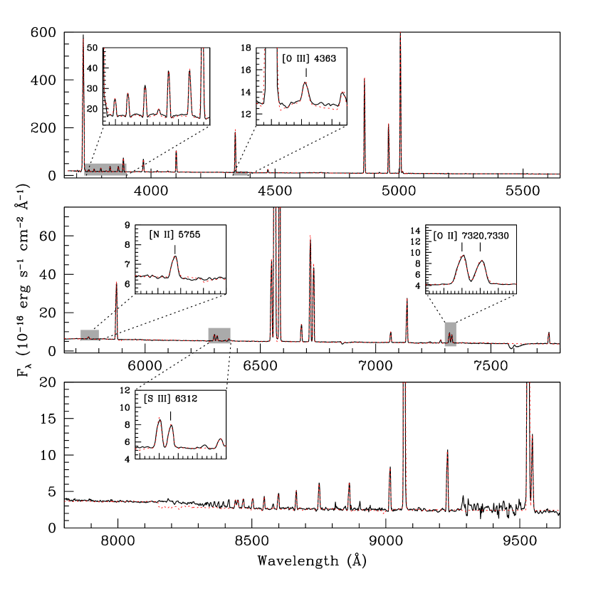
Figure 2.— Sample LBT spectrum of an H II region in NGC 628 with auroral line detections at a strength of 3$\sigma$ or greater. The spectrum is broken up into three sections: The top panel is the blue region, where the high quality of the spectrum is evident by the high signal to noise Balmer series (highlighted in the expanded box). The middle panel corresponds to the middle portion of the spectrum and the bottom panel to the red region of the spectrum. The strength of the auroral lines used in this paper [O III] $\lambda 4636$, [N II] $\lambda 5755$, [S III] $\lambda 6312$, and [O II] $\lambda\lambda 7320,7330$) are highlighted in the corresponding expanded boxes.

2.3. Emission Line Measurements

Emission line strengths are measured using various existing tools described in Croxall et al. (2013). The underlying continuum of our MODS1 spectra are modeled using the STARLIGHT spectral synthesis code (Fernandes et al., 2005). We fit Bruzual et al. (2013) models to the blue continuum red-ward of the [O II] $\lambda$3727 line, after masking nebular emission lines and Wolf-Rayet features, using a Calzetti et al. (2000) reddening law. Subsequently, emission lines are fit simultaneously with stellar and nebular continuum components. When automatically fitting emission lines, we initially assume these lines are well described by a Gaussian profile. Once continuum levels and line locations are measured, the final emission line values are computed by integrating the flux over each profile width. This step is important with respect to the high resolution of MODS data, because nebular structure can be seen in the emission line profiles such that they are not well-characterized by a Gaussian function. To ensure that noise spikes and multiple features within the same line are not mis-identified and fit, emission lines are required to have the same bulk kinematics and FWHM. We validate the automated line fits by measuring integrated fluxes by hand using the SPLOT routine within IRAF for all 62 extracted one-dimensional spectra. This exercise confirms the reliability of the automated method.

In the past, standard errors associated with a given line strength often followed a relatively simple, generalized prescription (e.g., Skillman et al., 1994). Here, the error associated with each line detection is a combination of the measured variance extracted from the two-dimensional variance image, the error associated with the sensitivity function, the Poisson noise in the continuum, the read noise of the detector, sky noise, a flat fielding calibration error, the error in the continuum placement, and uncertainty associated with reddening. For weak lines, the uncertainty is dominated by error from the continuum subtraction, whereas the lines with flux measurements much stronger than the rms noise of the continuum have errors dominated by error in flux calibration and reddening. To account for the inherent uncertainty in the flux calibration based on standard star observations (Oke, 1990), a minimum uncertainty of 2% is added in quadrature to the emission line flux uncertainties. Note that this is a conservative estimate as the use of HST has allowed improved calibrations of flux standards in CALSPEC (Bohlin, 2010). The minimum 2% emission line uncertainty forces a floor of $\sim$ 50 K uncertainty for the electron temperature calculations.

In this study, we focus on the most reliable spectra wherein at least one temperature-sensitive auroral line or doublet (i.e., [O III] $\lambda$4363, [N II] $\lambda$5755, [S III] $\lambda$6312, or [O II] $\lambda\lambda$7320,7330) is detected at a line strength $>3\sigma$. Note that this criterion is enforced to ensure that, despite best spectral reduction practices, contamination from other lines, continuum noise, remnant dichroic effects, etc. do not lead to false auroral line detections. In addition to this precaution, each auroral line is examined by eye to ensure no valid detections are excluded and no suspicious detections pass the cut. By this criterion, out of 62 observed H II regions, we detect at least one auroral line in 45 spectra.

2.4. Reddening Corrections

The relative intensities of the Balmer lines are nearly independent of both density and temperature, so they can be used to solve for the reddening. The spectra are de-reddened using an iterative application of the reddening law of O’Donnell (1994), parametrized by $A_{V}=3.1\ E(B-V)$. An initial reddening estimate is determined from the Balmer line ratios assuming a temperature of $T_{e}=10^{4}$ K and a density of $n_{e}=10^{2}$ cm^-3. Using this reddening, we determine an initial estimate of the electron temperature, which is an error weighted average of the electron temperatures calculated from the auroral lines. This new electron temperature is then used iteratively to modify the input assumptions for the reddening code until the average electron temperature changes by less than 20 K. The final reddening estimate is an error weighted average of the individual reddening values determined from the H$\delta$/H$\beta$, H$\gamma$/H$\beta$, and H$\alpha$/H$\beta$ ratios. As the lines are fit simultaneously with stellar population models, further corrections for underlying Balmer absorption are unnecessary.

Following Lee & Skillman (2004), the reddening value can be converted to the logarithmic extinction at $H\beta$ as C(H$\beta)=1.43E(B-V)$. Because of its high Galactic latitude, the foreground extinction for NGC 628 is expected to be low, with an approximate value of C(H$\beta$) = 0.10 (Schlafly & Finkbeiner, 2011). For NGC 628 we find a range in C(H$\beta$) of $\sim 0.0$ to 0.6. Because the MODS spectra extend out to the 1 µm cutoff, we observe the Paschen series and so perform an independent calculation of the reddening parameter which confirms the Balmer determinations.

Reddening corrected line intensities measured from the observed H II regions in the target fields are reported in Table 3 (the full table is available online). Various optical emission line ratios can be used to distinguish emission regions which are excited by different mechanisms (e.g., Baldwin et al., 1981). All 45 regions in the CHAOS sample clearly lie within the typical ranges observed for H II regions, ruling out contributions from active galactic nuclei and supernovae remnants, and allowing the standard direct analysis of physical conditions in H II regions.

Table 3 Emission-Line Intensities and Equivalent Widths for LBT Observations of H II regions in NGC 628

	$I(\lambda)/I(\mbox{H}\beta)$
Ion	-35.9+57.7	+49.8+48.7	-73.1-27.3	-76.2+22.9	-36.8-73.4	+68.5+53.4	+81.6-32.3
H14 $\lambda$3721	0.020$\pm$0.001	0.022$\pm$0.001	0.012$\pm$0.001	0.018$\pm$0.003	0.015$\pm$0.001	0.012$\pm$0.002	0.015$\pm$0.001
[O ii] $\lambda$3726	0.475$\pm$0.009	0.694$\pm$0.018	0.492$\pm$0.010	0.507$\pm$0.022	0.472$\pm$0.009	0.626$\pm$0.013	0.352$\pm$0.007
[O ii] $\lambda$3728	0.565$\pm$0.011	0.959$\pm$0.020	0.642$\pm$0.013	0.658$\pm$0.022	0.778$\pm$0.016	0.784$\pm$0.016	0.580$\pm$0.012
H13 $\lambda$3734	0.025$\pm$0.001	0.027$\pm$0.001	0.015$\pm$0.001	0.022$\pm$0.003	0.019$\pm$0.001	0.015$\pm$0.003	0.019$\pm$0.001
H12 $\lambda$3750	0.034$\pm$0.002	0.037$\pm$0.003	0.015$\pm$0.001	0.027$\pm$0.008	0.015$\pm$0.003	0.019$\pm$0.006	0.017$\pm$0.001
H11 $\lambda$3770	0.045$\pm$0.001	0.049$\pm$0.003	0.035$\pm$0.001	0.036$\pm$0.008	0.027$\pm$0.003	0.023$\pm$0.006	0.036$\pm$0.001
H10 $\lambda$3797	0.054$\pm$0.001	0.058$\pm$0.003	0.034$\pm$0.001	0.048$\pm$0.008	0.041$\pm$0.003	0.031$\pm$0.005	0.041$\pm$0.001
He I $\lambda$3819	0.007$\pm$0.001	0.016$\pm$0.003	0.003$\pm$0.001	$<\sim$0.022	$<\sim$ 0.007	0.024$\pm$0.005	0.010$\pm$0.001
H9 $\lambda$3835	0.070$\pm$0.001	0.082$\pm$0.003	0.064$\pm$0.001	0.068$\pm$0.007	0.079$\pm$0.002	0.075$\pm$0.005	0.067$\pm$0.001
[Ne iii] $\lambda$3868	$<\sim$ 0.004	0.012$\pm$0.002	0.006$\pm$0.002	$<\sim$ 0.023	$<\sim$ 0.007	0.017$\pm$0.003	$<\sim$ 0.003
He I $\lambda$3888	0.050$\pm$0.001	0.052$\pm$0.003	0.082$\pm$0.002	0.046$\pm$0.007	0.094$\pm$0.002	0.080$\pm$0.005	0.085$\pm$0.002
H8 $\lambda$3889	0.105$\pm$0.003	0.111$\pm$0.005	0.065$\pm$0.002	0.093$\pm$0.015	0.079$\pm$0.005	0.060$\pm$0.010	0.080$\pm$0.002
He I $\lambda$3964	0.008$\pm$0.001	0.013$\pm$0.002	0.008$\pm$0.001	$<\sim$ 0.021	$<\sim$ 0.006	0.013$\pm$0.004	$<\sim$ 0.003
[Ne iii] $\lambda$3967	…	$<\sim$ 0.009	0.069$\pm$0.008	$<\sim$ 0.019	$<\sim$ 0.056	$<\sim$ 0.076	$<\sim$ 0.020
H7 $\lambda$3970	0.156$\pm$0.004	0.163$\pm$0.007	0.098$\pm$0.003	0.138$\pm$0.022	0.116$\pm$0.007	0.087$\pm$0.015	0.120$\pm$0.003
[Ne iii] $\lambda$4011	…	$<\sim$ 0.004	…	…	$<\sim$ 0.005	…	0.008$\pm$0.001
He I $\lambda$4026	0.011$\pm$0.001	0.019$\pm$0.002	0.010$\pm$0.001	$<\sim$ 0.014	0.011$\pm$0.001	$<\sim$ 0.008	0.017$\pm$0.001
[S ii] $\lambda$4068	0.007$\pm$0.001	0.011$\pm$0.001	0.011$\pm$0.001	$<\sim$ 0.012	$<\sim$ 0.004	0.014$\pm$0.003	$<\sim$ 0.002
[S ii] $\lambda$4076	0.003$\pm$0.001	0.008$\pm$0.001	0.006$\pm$0.001	$<\sim$ 0.012	…	$<\sim$ 0.008	…
H$\delta$ $\lambda$4101	0.247$\pm$0.005	0.271$\pm$0.005	0.275$\pm$0.006	0.253$\pm$0.005	0.276$\pm$0.006	0.288$\pm$0.006	0.250$\pm$0.005
He I $\lambda$4120	0.003$\pm$0.001	0.012$\pm$0.001	0.004$\pm$0.001	$<\sim$ 0.012	0.004$\pm$0.001	…	0.010$\pm$0.001
He I $\lambda$4143	0.004$\pm$0.001	$<\sim$ 0.003	…	$<\sim$ 0.011	$<\sim$ 0.003	$<\sim$ 0.006	0.002$\pm$0.001
H$\gamma$ $\lambda$4340	0.466$\pm$0.009	0.464$\pm$0.009	0.481$\pm$0.010	0.465$\pm$0.009	0.488$\pm$0.010	0.478$\pm$0.010	0.474$\pm$0.009
[O iii] $\lambda$4363	$<\sim$ 0.004	$<\sim$ 0.008	$<\sim$ 0.004	$<\sim$ 0.011	$<\sim$ 0.004	$<\sim$ 0.006	$<\sim$ 0.003
He I $\lambda$4387	0.006$\pm$0.001	0.008$\pm$0.001	0.007$\pm$0.001	$<\sim$ 0.010	0.011$\pm$0.001	0.014$\pm$0.002	0.010$\pm$0.001
He I $\lambda$4471	0.024$\pm$0.001	0.038$\pm$0.001	0.021$\pm$0.001	0.019$\pm$0.003	0.018$\pm$0.001	0.022$\pm$0.002	0.028$\pm$0.001
[Fe iii] $\lambda$4658	0.002$\pm$0.001	0.005$\pm$0.001	0.006$\pm$0.001	$<\sim$ 0.009	…	…	…
He II $\lambda$4685	0.007$\pm$0.001	0.021$\pm$0.001	0.010$\pm$0.001	$<\sim$ 0.009	0.003$\pm$0.001	0.006$\pm$0.002	0.022$\pm$0.001
H$\beta$ $\lambda$4861	1.000$\pm$0.020	1.000$\pm$0.020	1.000$\pm$0.020	1.000$\pm$0.020	1.000$\pm$0.020	1.000$\pm$0.020	1.000$\pm$0.020
He I $\lambda$4921	0.007$\pm$0.001	0.013$\pm$0.001	0.008$\pm$0.001	$<\sim$ 0.013	0.008$\pm$0.001	0.006$\pm$0.002	0.010$\pm$0.001
[O iii] $\lambda$4958	0.033$\pm$0.001	0.169$\pm$0.003	0.049$\pm$0.001	0.056$\pm$0.004	0.051$\pm$0.001	0.112$\pm$0.002	0.047$\pm$0.001
[O iii] $\lambda$5006	0.101$\pm$0.002	0.507$\pm$0.010	0.144$\pm$0.003	0.176$\pm$0.004	0.155$\pm$0.003	0.337$\pm$0.007	0.154$\pm$0.003
He I $\lambda$5015	0.015$\pm$0.001	0.020$\pm$0.001	0.013$\pm$0.001	$<\sim$ 0.012	0.013$\pm$0.001	0.009$\pm$0.002	0.015$\pm$0.001
NI $\lambda$5197	0.009$\pm$0.001	0.008$\pm$0.001	0.009$\pm$0.001	$<\sim$ 0.012	0.015$\pm$0.001	0.012$\pm$0.002	0.003$\pm$0.001
O I $\lambda$5577	0.003$\pm$0.001	$<\sim$ 0.004	$<\sim$ 0.002	$<\sim$ 0.015	$<\sim$ 0.003	…	0.004$\pm$0.001
[N ii] $\lambda$5754	0.004$\pm$0.001	0.006$\pm$0.001	$<\sim$ 0.001	0.006$\pm$0.001	0.005$\pm$0.001	0.008$\pm$0.001	$<\sim$ 0.001
He I $\lambda$5875	0.074$\pm$0.001	0.104$\pm$0.002	0.069$\pm$0.001	0.078$\pm$0.002	0.084$\pm$0.002	0.088$\pm$0.002	0.101$\pm$0.002
[O ı] $\lambda$6300	0.015$\pm$0.001	0.018$\pm$0.001	0.019$\pm$0.001	0.014$\pm$0.002	0.020$\pm$0.001	0.022$\pm$0.001	0.008$\pm$0.001
[S iii] $\lambda$6312	0.003$\pm$0.001	0.007$\pm$0.001	0.004$\pm$0.001	0.004$\pm$0.001	$<\sim$ 0.001	0.007$\pm$0.001	0.003$\pm$0.001
[O ı] $\lambda$6363	0.004$\pm$0.001	0.005$\pm$0.001	0.007$\pm$0.001	$<\sim$ 0.005	0.007$\pm$0.001	0.007$\pm$0.001	0.003$\pm$0.001
[N ii] $\lambda$6548	0.321$\pm$0.006	0.342$\pm$0.007	0.307$\pm$0.006	0.316$\pm$0.006	0.312$\pm$0.006	0.309$\pm$0.006	0.294$\pm$0.006
H$\alpha$ $\lambda$6562	3.095$\pm$0.062	3.029$\pm$0.061	3.103$\pm$0.062	3.063$\pm$0.061	3.105$\pm$0.062	3.074$\pm$0.061	3.182$\pm$0.064
[N ii] $\lambda$6583	1.008$\pm$0.020	1.055$\pm$0.021	0.957$\pm$0.019	0.987$\pm$0.020	0.977$\pm$0.020	1.025$\pm$0.020	0.898$\pm$0.018
He I $\lambda$6678	0.025$\pm$0.001	0.034$\pm$0.001	0.022$\pm$0.001	0.023$\pm$0.002	0.023$\pm$0.001	0.027$\pm$0.001	0.031$\pm$0.001
[S ii] $\lambda$6716	0.313$\pm$0.006	0.234$\pm$0.005	0.401$\pm$0.008	0.288$\pm$0.006	0.423$\pm$0.008	0.333$\pm$0.007	0.243$\pm$0.005
[S ii] $\lambda$6730	0.225$\pm$0.005	0.192$\pm$0.004	0.289$\pm$0.006	0.204$\pm$0.004	0.306$\pm$0.006	0.253$\pm$0.005	0.170$\pm$0.003
He I $\lambda$7065	0.010$\pm$0.001	0.020$\pm$0.001	0.013$\pm$0.001	0.009$\pm$0.001	0.010$\pm$0.001	0.017$\pm$0.001	0.014$\pm$0.001
[Ar iii] $\lambda$7135	0.028$\pm$0.001	0.069$\pm$0.001	0.026$\pm$0.001	0.034$\pm$0.001	0.025$\pm$0.001	0.057$\pm$0.001	0.036$\pm$0.001
He I $\lambda$7281	0.004$\pm$0.001	0.005$\pm$0.001	0.003$\pm$0.001	$<\sim$ 0.004	0.003$\pm$0.001	0.004$\pm$0.001	0.004$\pm$0.001
[O ii] $\lambda$7319	$<\sim$ 0.004	0.013$\pm$0.001	0.007$\pm$0.001	0.007$\pm$0.001	0.008$\pm$0.001	0.011$\pm$0.001	$<\sim$ 0.005
[O ii] $\lambda$7330	0.004$\pm$0.001	0.010$\pm$0.001	0.003$\pm$0.001	0.004$\pm$0.001	0.007$\pm$0.001	0.011$\pm$0.001	$<\sim$ 0.004
[Ar iii] $\lambda$7751	0.008$\pm$0.001	0.017$\pm$0.001	0.008$\pm$0.001	0.008$\pm$0.001	0.008$\pm$0.001	0.013$\pm$0.001	0.011$\pm$0.001
P18 $\lambda$8437	0.004$\pm$0.001	0.004$\pm$0.001	0.004$\pm$0.001	$<\sim$ 0.019	0.006$\pm$0.001	0.011$\pm$0.002	0.007$\pm$0.001
O I $\lambda$8446	0.006$\pm$0.001	0.007$\pm$0.001	0.011$\pm$0.001	$<\sim$ 0.020	0.007$\pm$0.001	…	…
P17 $\lambda$8467	0.004$\pm$0.001	0.005$\pm$0.001	0.008$\pm$0.001	$<\sim$ 0.019	0.004$\pm$0.001	$<\sim$ 0.005	0.006$\pm$0.001
P16 $\lambda$8502	0.006$\pm$0.001	0.006$\pm$0.001	0.009$\pm$0.001	$<\sim$ 0.020	0.005$\pm$0.001	$<\sim$ 0.005	0.005$\pm$0.001
P15 $\lambda$8545	0.007$\pm$0.001	0.007$\pm$0.001	0.012$\pm$0.001	$<\sim$ 0.019	0.006$\pm$0.001	$<\sim$ 0.005	0.007$\pm$0.001
P14 $\lambda$8598	0.007$\pm$0.001	0.008$\pm$0.001	0.013$\pm$0.001	$<\sim$ 0.020	0.007$\pm$0.001	0.008$\pm$0.002	0.008$\pm$0.001
P13 $\lambda$8665	0.009$\pm$0.001	0.011$\pm$0.001	0.017$\pm$0.001	$<\sim$ 0.021	0.009$\pm$0.001	0.008$\pm$0.002	0.010$\pm$0.001
N I $\lambda$8683	0.002$\pm$0.001	$<\sim$ 0.004	0.006$\pm$0.001	$<\sim$ 0.021	$<\sim$ 0.002	$<\sim$ 0.005	$<\sim$ 0.002
P12 $\lambda$8750	0.005$\pm$0.001	0.013$\pm$0.001	0.012$\pm$0.001	$<\sim$ 0.021	0.020$\pm$0.001	0.037$\pm$0.002	0.012$\pm$0.001
P11 $\lambda$8862	0.010$\pm$0.001	0.019$\pm$0.001	0.021$\pm$0.001	$<\sim$ 0.022	0.017$\pm$0.001	0.028$\pm$0.002	0.023$\pm$0.001
P10 $\lambda$9015	0.024$\pm$0.001	0.022$\pm$0.001	0.024$\pm$0.001	0.021$\pm$0.002	0.024$\pm$0.001	0.017$\pm$0.001	0.025$\pm$0.001
[S iii] $\lambda$9068	0.238$\pm$0.005	0.367$\pm$0.007	0.192$\pm$0.004	0.245$\pm$0.005	0.167$\pm$0.003	0.293$\pm$0.006	0.284$\pm$0.006
P9 $\lambda$9229	0.030$\pm$0.001	0.030$\pm$0.001	0.032$\pm$0.001	0.031$\pm$0.003	0.025$\pm$0.001	0.029$\pm$0.001	0.036$\pm$0.001
[S iii] $\lambda$9530	0.644$\pm$0.013	0.969$\pm$0.019	0.554$\pm$0.011	0.699$\pm$0.015	0.479$\pm$0.010	0.837$\pm$0.017	0.788$\pm$0.016
P8 $\lambda$9546	0.020$\pm$0.001	0.044$\pm$0.001	0.025$\pm$0.001	0.019$\pm$0.005	0.054$\pm$0.001	0.030$\pm$0.001	0.061$\pm$0.001
CHβ	0.297$\pm$0.013	0.450$\pm$0.013	0.221$\pm$0.013	0.250$\pm$0.013	0.433$\pm$0.013	0.542$\pm$0.013	0.148$\pm$0.013
FHβ	257.9$\pm$0.4	715.5$\pm$2.9	391.8$\pm$0.3	202.3$\pm$1.2	190.2$\pm$0.3	77.9$\pm$0.2	297.6$\pm$0.2
EWHβ	202.3	139.8	102.6	143.3	121.6	90.9	114.5
EWHα	1331.5	1109.7	647.0	826.5	910.7	666.0	863.8

Note. —  Emission line fluxes. Detections at a significance of less than 3 $\sigma$ are given as upper limits. Full table available online only.

3. Physical Conditions

3.1. Three-Zone Temperature Determinations

A simple H II region can be modeled by three separate volumes: a low-, intermediate-, and high-ionization zone. Accurate H II region abundance determinations require reliable electron temperature measurements for each volume. This is typically done by observing a temperature-sensitive auroral-to-strong-line ratio. The [O III] I($\lambda\lambda$4959,5007)/I($\lambda$4363) ratio is expected to reflect the temperature in the high ionization zone. Similarly, the [N II] I($\lambda\lambda$6548,6484)/I($\lambda$5755) and the [O II] I($\lambda\lambda$7320,7330)/I($\lambda$3726,3728) ratios are expected to reflect the temperature in the low ionization zone. S and Ar ions do not neatly separate into these two zones and thus require an intermediate ionization zone, which can be measured by the [S III] I($\lambda\lambda$9069,9532)/I($\lambda$6312) ratio. Since the redder [S III] lines can be affected by atmospheric absorption, we employ the theoretical ratio of $\lambda$9532/$\lambda$9069 = 2.51 to make an upward correction to the weaker of the two lines if a deviation of more than 2% from the theoretical ratio is observed.

Following the precedent of Bresolin et al. (2009a), we have adopted the current best set of atomic data from the literature as reported in Table 4. For the H II regions with detected auroral lines, we determine electron temperatures using the reddening corrected line-ratios and appropriate atomic data, assuming the ions are well-approximated by a 5-level atom. Once a direct electron temperature is determined, the physical conditions of the other zones are needed to complete the H II region picture. Garnett (hereafter G92; 1992) relates the direct temperatures of different ionization zones using photoionization models:

T[S iii] $$=0.83\times\mbox{T[O~{}{\sc iii}]}+1700\mbox{ K}$$ (1)

T[N ii] $$=0.70\times\mbox{T[O~{}{\sc iii}]}+3000\mbox{ K.}$$ (2)

These relationships are valid for temperatures typical of H II regions: $T_{e}$ = 2,000$-$18,000 K. Observational evidence supporting these relationships can be found in the literature. For example, Bresolin et al. (2009a) and Kennicutt et al. (2003b) find a tight correlation between H II region observations and the G92 T[S III] versus T[O III] relationship and Esteban et al. (2009) find a high correlation coefficient for the T[N II] versus T[O III] G92 model. With the assumption that T[N II] = T[O II], since N⁺ and O⁺ have comparable ionization energies, we now have the tools to determine temperatures in all three ionization zone for all ions.

3.2. Impact Of Updated Atomic Data

Recent updates to atomic data are of particular importance to this paper as changes in the Einstein A-coefficients for [S III] result in a systematic shift of T[S III] to cooler temperatures. In M101, Kennicutt et al. (2003b, hereafter K03) measured 16 regions with both T[O III] and T[S III] and found a tight correlation around relationship defined by G92. K03 used collision strengths for S⁺⁺ from Tayal & Gupta (1999) and Einstein A coefficients from Kauffman & Sugar (1986). Contemporaneously, Pérez-Montero & Díaz (2003) noted a T[S III]-T[O III] theoretical relationship that differs from the standard G92 relationship, where the departure is mostly due to introducing atomic data from Tayal & Gupta (1999). This is also a factor in the analysis by Binette et al. (2012), who use the abundances from Hägele et al. (2006) and Pérez-Montero et al. (2006), both of whom employ the [S III] collision strengths from Tayal & Gupta (1999). Since then, further derivations of atomic coefficients for S⁺⁺ have been published, such as the work of Froese Fischer et al. (2006), whose Einstein A-values we adopt. Mendoza & Bautista (2014) performed extensive computations of new collisional data sets for [O III], [O II], [N II], [S III], [S II], and [Ar III] and compared to other data sets of effective collision strengths computed within the past two decades. They found that statistical consistency amongst data sets is typically around $\sim 20-30\%$, where the inherent dispersion in forbidden transitions is due to the strong sensitivity of the the resonance contribution to the scattering numerical approach, target atomic model, energy mesh, and small interactions such as relativistic corrections. However, they note that with the exception of [S II], the resulting theoretical temperature dispersions have been found to be no larger than 10$\%$. Following the recommendations of Mendoza & Bautista (2014), and considering the discussion of effective collision strengths for [O III] by Storey et al. (2014), we adopt the most up-to-date atomic data (see Table 4).

To demonstrate the significance of atomic data updates, in Figure 3 we present a comparison of temperatures determined for the K03 M101 regions using (1) the atomic data as in KO3: specifically, Tayal & Gupta (1999) and Kauffman & Sugar (1986) for [S III], and (2) the current database adopted here (see Table 4). Temperatures determined with the old atomic data are plotted as open circles, while the updated values are closed circles, and the set of points belonging to the same H II region are connected. For reference, the one-to-one relation is plotted as a solid line and the theoretical relationship of G92 is shown as a short dashed line. The comparison in Figure 3 shows a shift of roughly 10% in T[S III] ($\sim$1000 K) in the sense that using the newer atomic data results in lower values of T[S III]. Additionally, in Figure 4 we plot the difference in electron temperature due to updating the atomic data versus the new electron temperature. The old temperatures are determined using the same atomic data as K03, whereas the new temperatures use the updated atomic data listed in Table 4. The temperature trends shown in Figure 4 show that the atomic data for [N II] and [O III] have remained fairly stable, whereas the data for [O II] and [S III] have not yet converged. As we will see in the next section, our observations show significant discrepancies between values of T[S III] and T[O III], in the sense that some T[O III] values are significantly higher.

3.3. Electron Temperature and Density Determinations

To establish a low-uncertainty electron temperature estimate, we define a quality criterion requiring a 3$\sigma$ detection of the auroral line measurement (see § 2.3). The high throughput of the MODS over a large optical and near-UV wavelength range allows us to take advantage of the following auroral lines: [S II] $\lambda\lambda$4068,4076, [O III] $\lambda$4363, [Ar III] $\lambda$5192, [N II] $\lambda$5755, [S III] $\lambda$6312, and [O II] $\lambda\lambda$7320,7330. In the NGC 628 spectra, there are very few [S II] $\lambda\lambda$4068,4076 and [Ar III] $\lambda$5192 detections, so we will focus on the four lines with the most numerous detections. We detect the following auroral line measurements at a strength of 3$\sigma$ or greater: [O III] $\lambda$4363 in 18 H II regions, [N II] $\lambda$5755 in 29 H II regions, [S III] $\lambda$6312 in 40 H II regions, and [O II] $\lambda\lambda$7320,7330 in 40 H II regions. Due to the previous concerns with [O II] temperature measurements (e.g., Kennicutt et al., 2003b), we do not report abundances calculated from this diagnostic. Rather, we defer to a future analysis of the entire CHAOS sample. The result is a sample of 45 H II regions with direct abundances from [O III], [N II], or [S III]; where 40 of these regions have multiple temperature determinations. The auroral lines measured for each H II region are listed in Table 2.

The [S II] $\lambda\lambda$6717,6731 ratio is used to determine the electron densities, which are confirmed with density determinations from the [O II] $\lambda\lambda$3726,3728 line ratio. For all densities which are consistent with the low density limit, abundance calculations assume $n_{e}=10^{2}$ cm^-3 (which is consistent with the 1$\sigma$ upper bounds and produces identical results for all lower values of $n_{e}$), else the derived higher electron density ($n_{e}>10^{2}$ cm^-3) is used. The electron temperature and density determinations are listed in Table 3.3 (full table is available online).

Table 4Sources of Updated Atomic Data for CHAOS

Ion	Radiative Transition Probabilities	Collision Strengths
[O II]	Froese Fischer & Tachiev (2004)⋆†	Kisielius et al. (2009)
[O III]	Froese Fischer & Tachiev (2004)⋆†	Storey et al. (2014)
[N II]	Froese Fischer & Tachiev (2004)⋆	Tayal (2011)
[Ne III]	Froese Fischer & Tachiev (2004)⋆	McLaughlin & Bell (2000)
[Ar III]	Mendoza & Zeippen (1983)	Munoz Burgos et al. (2009)
[S II]	Mendoza & Bautista (2014)	Tayal & Zatsarinny (2010)
[S III]	Froese Fischer et al. (2006)	Hudson et al. (2012)

Note. — The atomic data used by the 5-level atom approximation has been updated with current values from the literature as reported here.

^⋆ Agrees with updated values from Tayal (2011).

^† Equivalent to Tachiev & Froese Fischer (2002), as recommended by Stasińska et al. (2012).

Figure 3.— The effect of updating atomic data as demonstrated by comparisons of [O III] and [S III] temperature determinations for the H II regions in M101 from K03. Temperatures determined with the atomic dataset of K03 (specifically, Tayal & Gupta (1999) and Kauffman & Sugar (1986) for [S III]) are plotted as open circles, whereas values determined using the sources adopted here (see Table 4) are closed circles. Sets of points belonging to the same H II region are connected. For reference, the equivalence relation is plotted as a solid line and the theoretical relationship of G92 is shown as a short dashed line.

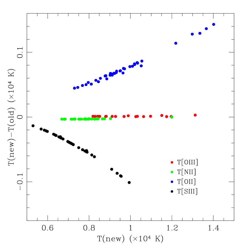
Figure 4.— The effect of updating atomic data as demonstrated by the difference of new and old electron temperatures versus new temperature. Data is color coded for each ion: T[O III] - red, T[N II] - orange, [O II] - green, and T[S III] - blue. Little difference is seen for T[N II] and T[O III], whereas significant updates have been made to the [S III] and [O II] atomic data and resulting temperatures.

Table 5Ionic and Total Abundances for MODS/LBT Observations of NGC 628

t(O₂)_measured (K) & … 9000$\pm$100 7300$\pm$100 7500$\pm$500 8200$\pm$100 9300$\pm$200
t(O₃)_measured (K) … … … … … …
t(N₂)_measured (K) 6800$\pm$100 7200$\pm$200 … 7300$\pm$400 7300$\pm$200 8100$\pm$300
t(S₃)_measured (K) 5700$\pm$100 6400$\pm$100 6400$\pm$100 6000$\pm$400 … 6600$\pm$200
$n_{e}$(_measured) (cm^-3) 57 248 59 37 64 126

t(O₂)_used (K) 6800$\pm$500 7200$\pm$200 6900$\pm$500 7300$\pm$400 7300$\pm$200 8100$\pm$300
t(O₃)_used (K) 4800$\pm$500 5700$\pm$500 5600$\pm$500 5200$\pm$500 6100$\pm$500 6000$\pm$500
t(N₂)_used (K) 6800$\pm$200 7200$\pm$200 6900$\pm$500 7300$\pm$400 7300$\pm$200 8100$\pm$300
t(S₃)_used (K) 5700$\pm$200 6400$\pm$200 6400$\pm$200 6000$\pm$400 6800$\pm$500 6600$\pm$200
$n_{e}$(_used) (cm^-3) 100 248 100 100 100 126
O+/H+ (10⁵) 28.1$\pm$1.4 32.5$\pm$2.0 26.9$\pm$5.3 20.4$\pm$3.2 21.4$\pm$1.3 14.2$\pm$1.2
O++/H+ (10⁵) 11.7$\pm$3.8 22.1$\pm$5.2 6.58$\pm$1.55 12.9$\pm$3.9 4.44$\pm$0.90 11.3$\pm$2.4
12 + log(O/H) (dex) 8.60$\pm$0.04 8.74$\pm$0.04 8.52$\pm$0.07 8.52$\pm$0.07 8.41$\pm$0.03 8.41$\pm$0.05
N+/H+ (10⁶) 64.8$\pm$2.1 56.5$\pm$2.2 57.2$\pm$6.9 49.1$\pm$4.8 49.2$\pm$1.8 35.2$\pm$1.8
N ICF 1.417$\pm$0.161 1.680$\pm$0.200 1.245$\pm$0.318 1.635$\pm$0.361 1.207$\pm$0.101 1.796$\pm$0.240
log(N/O) (dex) -0.64$\pm$0.03 -0.76$\pm$0.03 -0.67$\pm$0.10 -0.62$\pm$0.08 -0.64$\pm$0.03 -0.61$\pm$0.04
12 + log(N/H) (dex) 7.96$\pm$0.05 7.98$\pm$0.05 7.85$\pm$0.12 7.90$\pm$0.10 7.77$\pm$0.04 7.80$\pm$0.06
S+/H+ (10⁷) 43.1$\pm$1.4 29.2$\pm$1.1 51.4$\pm$6.0 30.7$\pm$2.9 46.1$\pm$1.6 26.7$\pm$1.3
S++/H+ (10⁷) 178.$\pm$5.4 188.$\pm$4.4 104.$\pm$2.2 160.$\pm$17. 75.6$\pm$7.4 141.$\pm$5.3
S ICF 1.083$\pm$0.108 1.151$\pm$0.115 1.026$\pm$0.103 1.142$\pm$0.114 1.013$\pm$0.101 1.172$\pm$0.117
log(S/O) (dex) -1.22$\pm$0.06 -1.34$\pm$0.06 -1.32$\pm$0.09 -1.19$\pm$0.09 -1.32$\pm$0.06 -1.11$\pm$0.06
12 + log(S/H) (dex) 7.38$\pm$0.05 7.40$\pm$0.04 7.20$\pm$0.05 7.34$\pm$0.06 7.09$\pm$0.05 7.29$\pm$0.05
Ne++/H+ (10⁶) … 24.8$\pm$0.58 14.1$\pm$2.8 … … 26.9$\pm$0.63
Ne ICF 3.398$\pm$1.144 2.471$\pm$0.628 5.085$\pm$1.461 2.575$\pm$0.878 5.823$\pm$1.224 2.256$\pm$0.535
log(Ne/O) (dex) … -0.95$\pm$0.10 -0.67$\pm$0.13 … … -0.62$\pm$0.09
12 + log(Ne/H) (dex) … 7.79$\pm$0.11 7.85$\pm$0.15 … … 7.78$\pm$0.10
Ar++/H+ (10⁷) 14.7$\pm$0.53 21.5$\pm$0.56 9.08$\pm$0.22 13.3$\pm$2.0 7.02$\pm$0.83 14.9$\pm$0.69
Ar ICF 1.916$\pm$0.192 1.569$\pm$0.157 2.730$\pm$0.273 1.602$\pm$0.160 3.140$\pm$0.314 1.510$\pm$0.151
log(Ar/O) (dex) -2.15$\pm$0.06 -2.21$\pm$0.06 -2.13$\pm$0.08 -2.19$\pm$0.10 -2.07$\pm$0.07 -2.05$\pm$0.07
12 + log(Ar/H) (dex) 6.45$\pm$0.05 6.53$\pm$0.05 6.39$\pm$0.05 6.33$\pm$0.08 6.34$\pm$0.07 6.35$\pm$0.05

Note. — Electron temperatures and ionic and total abundances for objects with an [O III] $\lambda 4363$, [N II] $\lambda 5755$, or [S III] $\lambda 6312$ line signal to noise ratio of $3\sigma$ or greater. Electron temperatures were calculated using the [O III] ($\lambda 4959+\lambda 5007$)/$\lambda 4363$, [N II] ($\lambda 6548+\lambda 6584$)/$\lambda 5755$, or the [S III] ($\lambda 9069+\lambda 9532$)/$\lambda 6312$ diagnostic line ratio. Full table available online only.

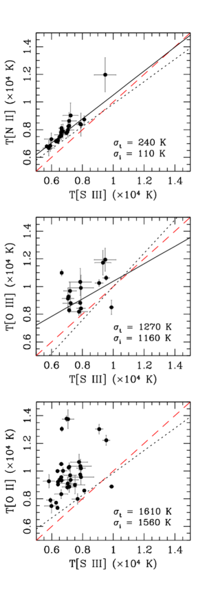
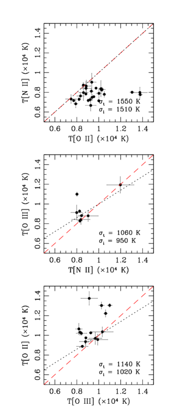
Figure 5.— Comparisons of the relations between the [O III], [N II], [O II], and [S III] $T_{e}$ temperatures for H II regions with more than one temperature measurement. The red long-dashed lines represent equal temperatures and black short-dashed lines are the G92 relationships. For the T[N II] versus T[S III] and T[O III] versus T[S III] panels, the error-weighted least-squares best fit is shown by solid lines. The total and intrinsic scatter around the line of equality is give for each comparison.

3.4. Comparing Electron Temperature Measurements

Using the 45 H II regions in our sample with multiple auroral line measurements, all of which were double checked by hand, we compare the calculated electron temperatures in Figure 5. The red dashed lines show the line of equality and the black short dashed lines are the expected relationships from the photoionization models calculated by G92. For each set of variables we calculate the scatter in the data, with errors in both coordinates, around the line of equality and determine how much can be attributed to a physically significant intrinsic scatter using the MPFITEXY (Williams et al., 2010) routine in IDL. The intrinsic scatter is determined by minimizing the departure of $\chi^{2}$/(degrees of freedom) from 1 by introducing an additional scatter term to the weighting of each data point. Additionally, in two cases we also perform a least-squares fit, which is shown with a solid line. The calculated total and intrinsic scatters, $\sigma_{t}$ and $\sigma_{i}$ respectively, are displayed in Figure 5.

The left column of Figure 5 shows T[N II], T[O III], and T[O II] as a function of T[S III]. The top panel of this column shows a very tight correlation between T[N II] and T[S III]. The dispersion in this relationship about the line of equality is 240 K, and is consistent with being due entirely to observational uncertainties (i.e., very little internal scatter). The middle panel shows a large scatter for the comparison of T[O III] and T[S III], with a dispersion around the line of equality of 1270 K, indicating an intrinsic dispersion of 1160 K. The bottom panel shows a comparison of the T[O II] and T[S III] measurements, where the scatter is, again, quite large at 1610 K, indicating an intrinsic dispersion of 1560 K. This panel is similar to the T[O III] versus T[S III] comparison in having both a large dispersion and a systematic offset to smaller T[S III] values.

The right column of Figure 5 compares T[N II], T[O III], and T[O II] to one another. The top panel shows T[N II] versus T[O II]. In this comparison, the scatter is again large, with a dispersion of 1550 K, indicating that essentially all of the dispersion is intrinsic (formally 1510 K). In this comparison, where roughly equal temperatures are expected from photoionization models, the data appear to fall into two groups. Roughly half of the data are shifted from the equality relationship by $\sim 1400$ K toward higher T[O II]. The other half of the data show an even larger offset in the sense that the T[O II] are hotter than the T[N II] estimates. Of the outliers, three fall into a group where the average offset is close to 4000 K. Most of the very large dispersion is due to this triad of outlying points. Overall, T[O II] is systematically larger than both T[N II] and T[S III] as noted in previous studies (e.g., Pilyugin et al., 2009; Esteban et al., 2009). The middle panel shows T[O III] versus T[N II]. Although there are only eight points in this comparison, all but one of the measurements are in agreement with the expected relationship from G92. Finally, in the bottom panel, the comparison between T[O II] and T[O III] shows a large dispersion of 1140 K, of which 1020 K is due to intrinsic scatter. These points show a similar trend to that seen in the T[O II]$-$T[S III] comparison, with preferential scatter to higher values of T[O II].

The magnitude of the scatter in the T[O III]$-$T[S III] relationship came as a surprise. In fact, the CHAOS program was designed around the assumption that a secure measurement of T[O III] implied a secure abundance (with the understanding that there could be small biases due to temperature inhomogeneities). Hägele et al. (2006) and Pérez-Montero et al. (2006) have both shown a poor correlation between T[O III] and T[S III], and Binette et al. (2012) showed definitively that discrepancies between T[O III] and T[S III] are very common in the sense that T[O III] is higher than T[S III]. We showed in Section 3.2 that recent updates to atomic data enhances the T[O III]-T[S III] discrepancy by uniformly shifting [S III] temperatures cooler, but cannot be entirely responsible for the magnitude of discrepancies observed. Although many of the points in NGC 628 are consistent with the equality trend or the relationship derived by G92, there are a significant number of outliers, in agreement with the trend noted by Binette et al. (2012). This large number of outliers, and the similar trends noted in the literature, call into question the reliability of [O III] as a temperature indicator in H II regions. We discuss the discrepant temperature measurements further in Section 5.1.

In sum, the T[N II] and T[S III] measurements appear to be generally consistent, especially for T${}_{e}<10^{4}$ K, while the T[O III] and T[O II] measurements are often discrepant. Because a significant fraction of the T[O III] and T[O II] measurements appear to be biased to higher than expected values, abundances based on the these temperature measurements exhibit both larger dispersions and systematic offsets. These results guide our chosen methodology for deriving abundances in Section 4.1.

4. A Homogeneous Abundance Analysis Based on [S III] and [N II] Temperatures

4.1. Methodology for Ionic and Absolute Abundance Calculations

From the comparisons in Section 3.4, it is clear that there are significant temperature measurement discrepancies. Because T[N II] and T[S III] show a very good correlation at low temperatures, we interpret this to mean that these temperatures are free from whatever systematic effects are affecting the T[O III] and T[O II] measurements. Fortunately, the vast majority of our sample have measurements of T[N II] or T[S III] (or both). Thus, we calculate absolute and relative abundances based primarily on temperatures determined from T[N II] and/or T[S III] in conjunction with the G92 scaling relationships for the other ionization zones. Specifically, when T[N II] and T[S III] are both measured, T[N II] is used for the low ionization zone, T[S III] is used for the intermediate zone, and T[S III] in combination with the G92 relationship is used for the high ionization zone. In the cases with only one temperature measurement, the temperatures in the other zones are inferred from the G92 relationships. Since we have [S III] or [N II] temperatures for 43 of the 45 H II regions, we can adopt this relatively homogeneous method for nearly the entire dataset. We base the subsequent analysis on this prioritization. For completeness, we present an abundance analysis based on T[O III] in Appendix A.

Ionic abundances relative to hydrogen are calculated using:

$${\frac{N(X^{i})}{N(H^{+})}\ }={\frac{I_{\lambda(i)}}{I_{H\beta}}\ }{\frac{j_{H\beta}}{j_{\lambda(i)}}\ }.$$ (3)

The emissivity coefficients, $j_{\lambda(i)}$, which are functions of both temperature and density, are determined using a 5-level atom approximation with the updated the atomic data reported in Table 4.

Total oxygen abundances (O/H) are calculated from the simple sum of O⁺/H⁺ and O⁺⁺/H⁺. The other abundance determinations require ionization correction factors (ICF) to account for unobserved ionic species. For nitrogen, we employ the common assumption that N/O = N⁺/O⁺ (Peimbert, 1967). This allows us to directly compare our results with other studies in the literature. Nava et al. (2006) have investigated the validity of this assumption, and concluded that it is valid at a precision of about 10%.

Collisionally excited emission lines of sulfur, neon, and argon are also observed in many of our spectra. For Ne we use a fairly straightforward ICF: ICF(Ne) = (O⁺ + O⁺⁺)/O⁺⁺ (Crockett et al., 2006). S and Ar present more complicated situations as both S⁺⁺ and S⁺⁺⁺ lie in the O⁺⁺ zone and Ar⁺⁺ spans both the O⁺ and the O⁺⁺ zones. Thuan et al. (1995) provide analytic ICF approximations for both S and Ar using the model calculations of photoionized H II regions by Stasińska (1990). We employ these ICFs from Thuan et al. (1995) to correct for the unobserved S⁺³, Ar⁺², and Ar⁺⁴ states:

ICF(S) $$=\frac{\mbox{S}}{\mbox{S}^{+}+\mbox{S}^{++}}$$

$$=\big{[}0.013+x\{5.10+x[-12.78+x(14.77-6.11x)]\}\big{]}^{-1}$$ (4)

ICF(Ar) $$=\frac{\mbox{Ar}}{\mbox{Ar}^{++}+\mbox{Ar}^{+++}}$$

$$=\{0.99+x[0.091+x(-1.14+0.077x)]\}^{-1}$$ (5)

$$=\frac{\mbox{Ar}}{\mbox{Ar}^{++}}=[0.15+x(2.39-2.64x)]^{-1},$$ (6)

where $x=$ O⁺/O and the second Ar equation is used when [Ar IV] $\lambda 4740$ emission is not observed. Ionic and total abundances are listed for 45 H II regions in NGC 628 in Table 3.3.

4.2. Alpha-Element Relative Abundances

$\alpha$-elements are thought to be produced in massive stars such that sulfur, neon, and argon are produced in parallel with oxygen (e.g., Woosley & Weaver, 1995). Figure 6 shows the sulfur, neon, and argon abundances measured for NGC 628 versus oxygen abundance. Error-weighted least-squares fits produce gradients within one standard deviation of a flat (zero) slope, and so we adopt the error-weighted average alpha-element abundances as constants, which are shown in Figure 6 as shaded boxes spanning one standard deviation. The sample covers a range of 8.0 $<$ 12+log(O/H) $<$ 9.0 with no obvious trends in sulfur, neon, or argon abundance. S/O, Ne/O, and Ar/O all show very small intrinsic dispersions of 0.08, 0.08, and 0.02 dex, respectively. We report average $\alpha$-element to oxygen abundance ratios in Table 6. In general, we find that the relative abundances of the $\alpha$-elements in NGC 628 behave as expected for the nucleosynthetic products of massive stars. The constant values over the range in metallicity are consistent with a universal value for the upper mass IMF. This is in agreement with the recent study of the IMF in M31 clusters by Weisz et al. (2015).

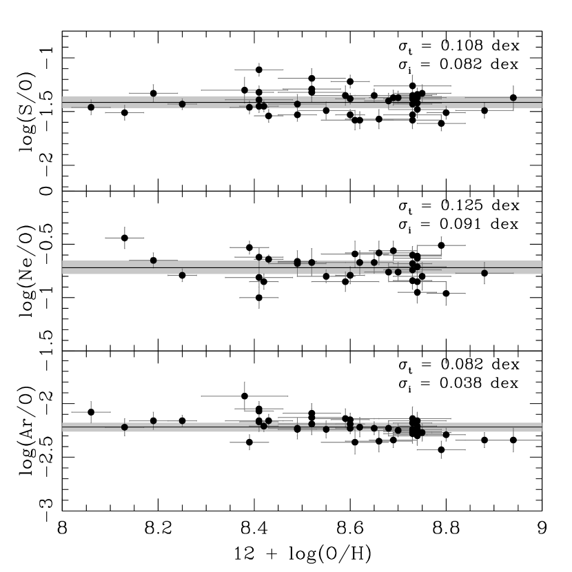
Figure 6.— $\alpha$-elements are plotted versus oxygen abundance for NGC 628. The error-weighted average $\alpha$-element abundance is illustrated in each panel by a shaded box centered on the average and extended to $\pm 1\sigma$. The measured dispersions and calculated intrinsic dispersions are indicated in the upper right of each panel. All three panels demonstrate constant $\alpha$-element/O ratio trends with small dispersions.

4.3. Radial Gradients in N/O and O/H

We display the derived N/O and O/H abundances in Figure 7 as a function of galactocentric radius. Because the locations of individual H II regions are known with high precision relative to one another, we consider only the uncertainties associated with oxygen abundance here. We characterize the N/O observations with a single, linear, error-weighted least-squares fit (solid line):

$$\log(\mbox{N/O})$$

$$=(-0.523\pm 0.034)+(-0.077\pm 0.006)\times{R}\ \mbox{ (dex/kpc)}$$

$$=(-0.521\pm 0.035)+(-0.849\pm 0.064)\times{R}\ \mbox{ (dex/}R_{25}),$$ (7)

with a measured dispersion in log(N/O) of $\sigma$ = 0.083 dex. Although this dispersion is small, the statistical analysis shows that most of this dispersion is intrinsic ($\sigma_{i}$ = 0.060 dex).

The bottom panel of Figure 7 shows the values of O/H as a function of galactocentric radius. The resulting best fit to the 45 objects in the sample is given by:

$$12+\log(\mbox{O/H})$$

$$=(8.834\pm 0.069)+(-0.044\pm 0.011)\times{R}\mbox{ (dex/kpc)}$$

$$=(8.835\pm 0.069)+(-0.485\pm 0.122)\times{R}\mbox{ (dex/}R_{25}),$$ (8)

with a dispersion in log(O/H) of $\sigma$ = 0.165 dex. Accounting for the observational uncertainties results in an intrinsic dispersion of 0.159 dex. This is significantly larger than the dispersions seen in the relative abundances. Since it is conceptually difficult to produce significant dispersions in absolute abundances without significant dispersions in relative abundances (due to time delays of delivery and mixing timescales), it is possible that this relatively large dispersion could be due to discrepant temperatures. The final CHAOS gradients are tabulated in Table 6.

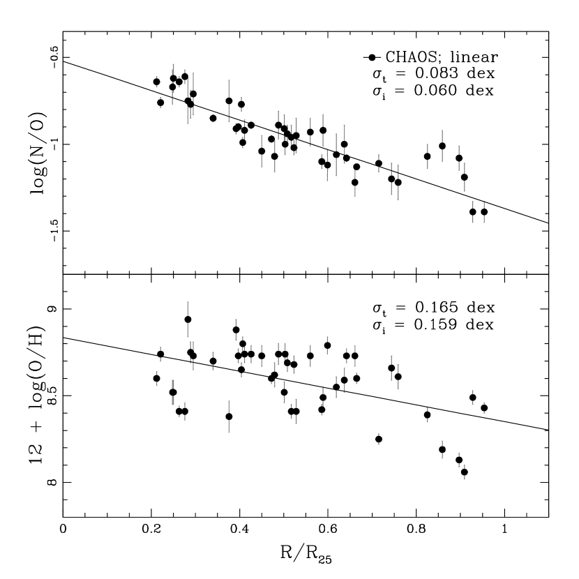
Figure 7.— N/O and O/H plotted versus galactocentric radius for NGC 628. The solid lines represent the least-squares linear fits to the data when considering the errors in N/O and O/H abundance respectively.

Table 6Adopted Abundance Gradients for NGC 628

y		x	Equation of Correlation	$\sigma_{t}$	$\sigma_{i}$
12+log(O/H)	vs.	$R$ (dex/kpc)	y = (8.834$\pm$0.069) + (-0.044$\pm 0.011)\times$X	0.165	0.159
		$R$ (dex/$R_{25}$)	y = (8.835$\pm$0.069) + (-0.485$\pm 0.122)\times$X
log(N/O)	vs.	$R$ (dex/kpc)	y = (-0.523$\pm$0.034) + (-0.077$\pm 0.005)\times$X	0.083	0.060
		$R$ (dex/$R_{25}$)	y = (-0.521$\pm$0.035) + (-0.849$\pm 0.064)\times$X
log(S/O)	vs.	12+log(O/H)	y = -1.413	0.108	0.082
log(Ne/O)	vs.	12+log(O/H)	y = -0.714	0.125	0.091
log(Ar/O)	vs.	12+log(O/H)	y = -2.219	0.082	0.038

Note. — The adopted best fits to the abundance gradients measured for the 3$\sigma$ NGC 628 CHAOS data.

5. DISCUSSION

5.1. Discrepant Temperature Measurements

5.1.1 Suspect [O III] Temperatures

Historically, [O III] $\lambda 4363$ is the best studied direct temperature auroral line, owing to its relative ease of observation, abundance of emitting ions, and increasing strength in the moderate- to low-metallicity H II regions of nearby dwarf and (all but the central regions of) spiral galaxies. Other common temperature-sensitive ratios, such as [N II] I($\lambda\lambda 6548,6584$)/I($\lambda 5755$), [O II] I($\lambda\lambda 7320,7330$)/I($\lambda\lambda 3726,3628$), and [S III] I($\lambda\lambda 9069,9532$)/I($\lambda 6312$), are limited by their weaker abundances, origination in the smaller low-ionization zone, and combination of optical and near-infrared line ratios. Because of these factors, the intensity ratio [O III] $\lambda 4363$/$\lambda\lambda$(4959+5007) has long been the chief diagnostic of nebular gas temperature.

In theory, the temperature measurements shown in Figure 5 should fall along the lines of the relationships from the photoionization models of G92, but in many regards they do not. Kennicutt et al. (2003b) raised concerns about T[O II], and additional studies have pointed out other significant temperature discrepancies (e.g., Bresolin et al., 2005; Pilyugin et al., 2009; Esteban et al., 2009; Zurita & Bresolin, 2012; Binette et al., 2012). For the CHAOS data, Figure 5 demonstrates a surprisingly large dispersion for T[S III] versus T[O III], yet a tight relationship for T[N II] versus T[S III]. We investigate these two relationships further here.

We reproduce the CHAOS T[N II]$-$T[S III] data in the left panel of Figure 8. As mentioned earlier, the dispersion in this relationship about the line of equality is small. K03 not did see such a tight relationship, but there were only 7 H II regions with measurements of both T[N II] and T[S III]. The K03 observations have been added to Figure 8 for comparison. For consistency, the K03 temperatures are recalculated using the K03 emission line fluxes and our adopted atomic data. The least-squares fit to the combined set sees an increase in the dispersion due to the additional scatter at higher temperatures. A very tight relationship between these two temperature diagnostics has been noted before (e.g., Bresolin et al., 2005; Zurita & Bresolin, 2012; Binette et al., 2012). The emergence of an excellent correlation indicates that T[N II] and T[S III] provide highly consistent measurements of H II region temperatures and increases confidence in their reliability at low temperatures.

In the right panel of Figure 8 we plot the CHAOS T[O III]$-$T[S III] measurements and compare them to the K03 data. K03 found excellent agreement between T[O III]$-$T[S III] measurements and the expectation from the photoionization modeling of G92. Our observations of NGC 628, coupled with updated atomic data, are at odds with the M101 study, showing a significant dispersion in the T[O III]$-$T[S III] comparison. The least-squares fit to the combined data set results in a total dispersion of 1090 K which corresponds to an intrinsic uncertainty of 950 K. As shown in Figure 3, the original K03 [S III] temperatures are higher by about 10%. The result is a shift in the T[O III]$-$T[S III] relationship away from the G92 relationship, and is equivalent to the offset observed for the CHAOS data. Pérez-Montero et al. (2006) suggest a theoretical T[O III]$-$T[S III] relationship that also differs from the G92 standard, identifying new atomic coefficients as the source of the difference. However, the new atomic data have minimal effect on the observed dispersions. One very important thing to note from Figure 8 is the difference in the temperature ranges covered by the observations in the two plots. The left hand panel concentrates on a tight correlation for values of T[N II] below $\sim$ 9,000 K, while the bulk of the T[O III] values in the right hand panel, which show significant scatter, are above $\sim$ 7,000 K. Thus, the conclusions from K03 and the present study could be understood as an increasing dispersion in the T[O III]$-$T[S III] relationship with decreasing temperature. This result appears to be supported by the right hand panel of Figure 8.

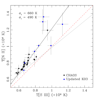
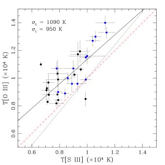
Figure 8.— Comparisons of the relations between T[N II] and T[O III] versus T[S III]. The lines and solid points are the same as in Figure 5. A parallel comparison is provided by the M101 direct measurements of Kennicutt et al. (2003b), where the open blue points correspond to the temperature values presented in their work and the closed blue points represent electron temperatures recalculated from their emission line fluxes with the adopted updated atomic data.

5.1.2 Sources of Temperature Discrepancies

We now turn to the possible causes of the significant temperature discrepancies demonstrated by Figures 5 and 8. Due to the moderately-high resolution of MODS, [O III] $\lambda 4363$ is resolved from the Hg $\lambda 4358$ sky line. Additionally, we examine the [O III] auroral line emission by hand in both the one-dimensional and two-dimensional spectra, eliminating concerns of cosmic rays, Balmer absorption, or other measurement errors. Recently, Binette et al. (2012) have highlighted the discrepancy between the T[O III] and T[S III] temperatures and investigated possible sources of this disagreement: temperature inhomogeneities, metallicity inhomogeneities, a non-Maxwell-Boltzmann distribution of electron energies, and shocks. Temperature inhomogeneities within individual H II regions were first proposed by Peimbert (1967), where non-uniform temperature distributions tend to result in average observed temperatures biased higher than true local temperatures. However, Binette et al. (2012) found that simple temperature fluctuations are insufficient to account for the magnitude of the T[O III]$-$T[S III] disparity, especially at the low electron temperatures characteristic of high abundance H II regions (see their Figure 4). Instead, Binette et al. conclude that metallicity inhomogeneities (e.g., Tsamis et al., 2003, 2011), adopting a $\kappa$-distribution for the electron energy distribution (Nicholls et al., 2012), and pollution by shock waves all successfully reproduce the observed T[O III] excesses (see their Figures $5-8$). However, Mendoza & Bautista (2014) found $\kappa$-distributions only account for observed temperature variations in low-excitation regions, and do not reconcile the differences in high-excitation regions.

For the low electron temperatures associated with the CHAOS data, Binette et al. (2012) demonstrate that plane-parallel shock models which propagate within a photoionized gas layer successfully bridge the T[O III]$-$T[S III] gap. The shocked nebula models show a diminishing excess of T[O III] with decreasing nebular metallicity (increasing T) similar to what we see in our data, where the largest excesses occur with decreasing temperature (increasing metallicity) towards the inner disk. By combining the continuous starburst model of Kewley et al. (2001) and the shock+precursor model of Allen et al. (2008), Binette et al. (2012) suggest an additional region which is a mixing zone of the photo- and shock-ionization zones.

In Figure 9 we reproduce the shock model data from Figure 8 of Binette et al. (2012) and compare the CHAOS data for NGC 628. The solid points are the H II regions which have both measured [O III] and [S III] temperatures, and are color coded by abundance. Points in this plot show that (with the exception of one major outlier: NGC 628-168.2+150.8) T[O III] is in excess of T[S III], where increased temperatures subsequently lead to artificially low oxygen abundances. This idea is congruent with the picture shown in Figure 9: the colors of the points indicate that their abundances are higher than those of the models to which they are closest. If their true photoionized T[O III] is lower ($\sim$T[S III] ), then the true oxygen abundance is higher and in better agreement with the model abundances.

It is clear from studies in the literature and from our CHAOS observations of NGC 628 that emission line spectra for some H II regions are affected by one or more processes which lead to discrepant temperatures derived from auroral line observations. By comparing the present observations with theoretical models, we have shown that shocks, as an example, can contribute to discrepant temperatures; however, the true nature of the perturbations is not clear. It is interesting to note that the auroral lines with the highest excitation energies (e.g., [O III] $\lambda 4363$ and [O II] $\lambda\lambda 7320,7330$, with excitation energies of 5.3 and 5.0 eV respectively) show the largest discrepancies, while those with lower excitation energies (e.g., [N II] $\lambda 5755$ and [S III]$\lambda 6312$, with excitation energies of 4.1 and 3.3 eV respectively) are less sensitive to these perturbations. The higher excitation energies of the oxygen temperature diagnostic lines may contribute to making these lines more vulnerable to the perturbations, regardless of the physical cause. This leads quite naturally to the result that the biases are larger in higher abundance (lower temperature) H II regions, in agreement with the observations. From the present NGC 628 dataset, we cannot deduce a single likely cause for the temperature discrepancies. However, in Appendix B we suggest relative Ar abundances as excellent diagnostics for identifying which spectra are most affected. We will revisit this problem with the entire CHAOS dataset.

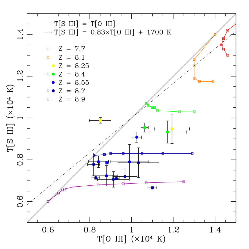
Figure 9.— T[O III] versus T[S III] plot for NGC 628 in comparison to models including the effects of shocks from Binette et al. (2012). Abundances are divided into bins and points are colored coded by the central oxygen abundance of each bin. Only points with measurements of both [S III] and [O III] temperatures are plotted as solid circles. The models of Binette et al. (2012), which combine the continuous starburst model of Kewley et al. (2001) and the shock+precursor model of Allen et al. (2008), are plotted as open squares.

5.2. Comparison of Gradients with Measurements from the Literature

Although NGC628 is one of the best-studied spiral galaxies, there are only a handful of previous studies with direct abundance measurements. We first perform a straightforward comparison to these studies, and then extend this comparison to the integral field spectroscopy study by Rosales-Ortega et al. (2011).

Three previous studies present direct abundance measurements for NGC 628: Berg et al. (2013, 14 regions, hereafter B13), Croxall et al. (2013, 7 regions, hereafter C13), and Castellanos et al. (2002, 1 region), but only the first reports nitrogen or $\alpha$-element abundance ratios. Note that the three studies derive electron temperatures using different methods. B13 used the [O III] and [N II] auroral lines to determine electron temperatures, Croxall et al. (2013) used the infrared [O III] $88$µm fine-structure line, and Castellanos et al. (2002) found agreement amongst four temperature determinations from the [O III], [S III], [N II], and [S II] auroral lines observed in one H II region. We have not attempted to make any corrections to place these different abundance derivations on a common scale.

5.2.1 Radial Gradients in N/O and O/H

The measure of nitrogen across NGC 628 offers further insight into the nature of abundance gradients. Because nitrogen and oxygen are formed primarily in intermediate- and high-mass stars respectively, they are returned to the interstellar medium on different time scales (e.g., Garnett, 1990; van Zee et al., 1998a, b; Berg et al., 2012). In the upper panel of Figure 10 we plot the CHAOS N/O gradient, including 11 observations with T[N II] measurements and three observations with T[O III] measurements from B13. The values from the literature are consistent with the trends established by the CHAOS observations; the main difference is the extension to greater radius afforded by the B13 points. Berg et al. (2013) used a likelihood ratio F-test to show that the N/O gradient is best described by a bi-modal relationship (short dashed line), where decreasing N/O flattens out near the isophotal radius (R${}_{25}\sim 11$ kpc,).

In the lower panel of Figure 10 we illustrate the oxygen abundance relationship across the disk of NGC 628. In comparison to the CHAOS data (solid points), direct abundances from B13 and C13 are plotted as open squares and open triangles respectively. The reduced level of scatter amongst sources when prioritizing T[S III] and T[N II] is confirmed when incorporating the additional points from the literature. Since the infrared fine-structure lines used by C13 are thought to produce abundances that are largely independent of electron temperature, the fact that these values lie in unison with the CHAOS data offer another confirmation of the chosen temperature determinations. Further, B13 measured T[N II] in 11 H II regions to obtain directly comparable abundances, and these values agree with the dispersion in the CHAOS sample. In short, this review of the oxygen abundance gradient with respect to a variety of temperature determinations supports our decision to conduct a homogeneous abundance analysis based on T[S III] and T[N II].

5.2.2 Comparison with Results from Rosales-Ortega (2011)

The most comprehensive emission line abundance survey of NGC 628 to date was carried out by Rosales-Ortega et al. (2011, hereafter RO11). The RO11 study performed a nearly complete 2D sampling of the disk within the isophotal radius, allowing a variety of statistically significant analyses. Complimentary to the work presented here, RO11 performed an in-depth comparison of various strong-line metallicity indicators and laid a framework of geometric parameters.

RO11 obtained robust 2D fiber spectroscopic observations of NGC 628, which were converted to a set of 96 H II region spectra which are directly comparable to the CHAOS observations. With this data set, different strong-line abundance estimators were used to explore the effects of choosing different calibrations. The RO11 ff-$T_{e}$ (Pilyugin, 2005) analysis of the H II region catalog mimics the data collection and analysis presented here, and allows the following side-by-side comparison.

In Figure 10 we compare N/O and O/H radial gradients from the ff-$T_{e}$ calibration of RO11. The top panel of Figure 10 illustrates the general agreement between the direct abundance and ff-$T_{e}$ N/O gradients for the optical disk. Within the uncertainty of measurement, the CHAOS best fit (Equation 7: log(N/O) = ($-0.523\pm 0.034$) + ($-0.077\pm 0.005)\times{R}$ (dex/kpc)) parallels the RO11 fit (log(N/O) = ($-0.50\pm 0.03$) + ($-0.080\pm 0.06)\times{R}$ dex/kpc), in particular, note that the gradients are within 1$\sigma$ of one another. Since the N/O ratio has little dependence on temperature, the two methods provide nearly identical results except for a small average shift. Note the outlined, shaded box displays the 0.3 dex spread in the measured data as reported by RO11. Similarly, the bottom panel of Figure 10 compares these two methods for the O/H gradient. With the addition of data from the literature extending into the outer disk (beyond $R_{25}$), RO11 propose a tri-modal oxygen abundance gradient: a steeply declining abundance gradient for the majority of the optical disk, with flatter features within the inner 2 kpc and in the outer disk. The mid O/H slope ($-0.034\pm 0.02$ dex/kpc) from RO11, extending from $\sim 0.1-0.7$ R/R₂₅, is shown as a grey shaded box in Figure 10 whose width represents the 1$\sigma$ error-weighted dispersion in the log(O/H) measurements. For this part of the optical disk, the RO11 results are in agreement with the slope from the CHAOS observations ($-0.044\pm 0.011$ dex/kpc), but are offset lower by $\sim 0.1$ dex. The CHAOS observations do not cover the inner or outer regions where RO11 find different slopes.

CHAOS Abundance Gradients for NGC 628

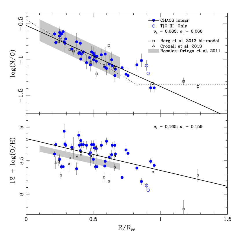
Figure 10.— N/O and O/H plotted versus galactocentric radius for NGC 628 and are compared to direct and ff-$T_{e}$ methods in the literature. Data from B13 (open squares) and from C13 (open triangles) are plotted, where electron temperatures were determined using [O III] and/or [N II] for the former and the infrared fine-structure [O III] $88\mu$ line for the latter. The solid line depicts the least-squares best fits to the CHAOS data, as reported in Section 4, whereas the shaded box represents the negative gradient and dispersion measured for the optical disk by RO11 using the ff-$T_{e}$ method. In the top panel, the CHAOS data intersects the bi-modal N/O relationship observed by B13 (dashed line). In the bottom panel, the [N II] based B13 data and the nearly temperature independent measurements of C13 coincide with the CHAOS data.

5.3. Dispersions in Abundances at a given Galactocentric Radius

The dispersion in abundances within the ISM of a galaxy is a very important observable, but there are very few galaxies with a sufficient number of observations to make statistically significant conclusions. Based on 61 direct [O III] $\lambda 4363$ measurements, Rosolowsky & Simon (2008, hereafter RS08) determined a significant dispersion in the oxygen abundance gradient of M33 ($\sigma_{i}=0.11$ dex). In this study, a number of parameters, including L(H$\alpha$), c(H$\beta$), Balmer absorption and emission equivalent widths, and ionization correction factor, were tested for correlated against the derived metallicity gradient and its residuals, but no trend indicative of systematic errors was found. The findings of RS08 were challenged by Bresolin (2011) using 8 observations of the [O III] $\lambda 4363$ auroral line and the $R_{23}$ strong-line method. Based on this analysis, Bresolin (2011) measured a much smaller dispersion, and speculated that the significant scatter seen in the $T_{e}$-based abundances of M33 from the RS08 sample is due to measurement errors in the weak [O III] $\lambda 4363$ auroral line.

Although relative abundances from the CHAOS observations show very small dispersions at a given galactocentric radius in NGC 628, the absolute oxygen abundances show a large and significant dispersion. RO11 also measured a large dispersion in metallicity, finding the scatter to be larger in their fiber-to-fiber sample (rms = 0.128 dex) than the H II region catalog (rms = 0.070 dex) (where several fiber spectra are averaged together). This level of spread is consistent with the CHAOS sample ($\sigma_{t}=0.165$ dex, $\sigma_{i}=0.159$ dex).

In Figure 11, we plot the average offset in O/H abundance from the best fit relationship in radial bins of 0.2 $R/R_{25}$ for both the CHAOS sample and the RO11 study. For the three bins in common between $0.2-0.8$ $R/R_{25}$, the RO11 data has both smaller average departures from the measured radial gradient and smaller dispersions around these mean offsets. This result further suggests that the large dispersion measured in the CHAOS gradient has a physical origin whose effect is removed when averaged over entire H II regions. Be that as it may, until the source(s) of the discrepant temperature measurements are better understood, at this point, it is best to consider the measured dispersion to be an upper limit.

In addition to temperature discrepancies, we investigate other sources of scatter in oxygen abundance, such as the symmetry of the metal abundance distributions, but find no obvious relationship with spatial structure (differences amongst spiral arms or arm versus inter-arm abundances) or ionization fraction. One advantage of the RO11 study over CHAOS is that it samples a nearly complete coverage of the disk. Since we have shown that the two studies find comparable oxygen abundance gradients, we can use the RO11 disk geometry analysis to complement our understanding of the CHAOS data. RO11 performed two detailed spatial analyses: (1) by quadrants and (2) by spiral arms, as defined by Kennicutt & Hodge (1980). RO11 found distinct radial trends in the ionization parameter and metallicity for both the geometrical quadrants and the morphological arms, indicating that the disk may have evolved somewhat asymmetrically. However, these variations result in O/H gradients which lie within the uncertainties of the overall abundance trend for the disk.

While the CHAOS and RO11 studies suggest the significant intrinsic oxygen abundance dispersion found for NGC 628 is real, a definitive source for such variation at a given radius has not been found. Further, considering the the contrasting results of the RS08 and Bresolin (2011) studies for M33, we speculate that these azimuthal variations are simply not recovered in small samples. For the large samples of direct abundances presented here and in RS08, the significant intrinsic dispersions measured are due to the electron temperatures. However, the dispersion could be due to discrepant temperatures, uncertainty in the measurements, or both. Following the line of argument laid out in Binette et al. (2012) and summarized in Section 5.1, the primary factor influencing temperature discrepancies, and subsequently determined abundances, is not yet clear.

Figure 11.— Average offset in oxygen abundance from the measured radial gradient plotted in radial bins of 0.2 dex for each the CHAOS sample and the RO11 study. Colored solid lines represent the average offset in each bin, where the extent of the shaded box depicts the dispersion around the mean offset.

6. SUMMARY AND CONCLUSIONS

The CHemical Abundances of Spirals (CHAOS) project seeks to establish a broader understanding of the chemical evolution of spiral galaxies in general. CHAOS harnesses the combined power of the Large Binocular Telescope (LBT) with the large spectral range and sensitivity of the Multi Object Double Spectrographs (MODS) to observe “direct” abundances in a large sample of H II regions in spiral galaxies. In this manner, we measure the largest sample of the highest quality spectra to date in NGC 628, with one or more temperature-sensitive auroral lines ([O III] $\lambda 4363$, [N II] $\lambda 5755$, and [S III]$\lambda 6312$) being observed at a strength of 3$\sigma$ or greater in 45 H II regions. Analysis of this data set provides the following insights:

1) Due to the obvious advantages in observing [O III] $\lambda 4363$ over the other auroral lines, it has long been the principle nebular temperature diagnostic. Further, the scarcity of observations of other lines in the literature has postponed any comparative tests of validity. The CHAOS sample presented here records multiple auroral lines in many of the H II regions observed, allowing a comparison of derived temperatures from multiple emission lines. We have shown a very tight relationship between temperatures based on [S III] $\lambda 6312$ and [N II] $\lambda 5755$ indicating that these temperatures are reliable. In contrast, temperatures from [O II] $\lambda\lambda 7320,7330$ and [O III] $\lambda 4363$ can often show large discrepancies compared to T[S III] and T[N II].

2) These results lead us to adopt a uniform method of electron temperature determination in which T[S III] and T[N II] are prioritized and used in combination with the theoretical relationships of G92. Through this approach, we were able to minimize the dispersion seen in the abundance gradients.

3) Relative abundances of S/O, Ne/O, and Ar/O, which are nearly independent of temperature, are measured to be constant across the entire optical disk of the galaxy. Using weighted least-squares fits, with errors in both the x and y variables, all three show very small intrinsic dispersions (0.08, 0.09, and 0.04 respectively). These unvarying values over the range in metallicity are consistent with a universal value for the upper mass range of the IMF.

4) Radial gradients are measured for both N/O and O/H out to the optical radius of NGC 628. The N/O ratios show a negative gradient, consistent with the previous works of Berg et al. (2013) and Rosales-Ortega et al. (2011), but do not sample the radial extent necessary to assess the presence of a bi-modal relationship. The small measured dispersion about the N/O relationship is attributed to intrinsic dispersion ($\sigma_{t}=0.083$; $\sigma_{i}=0.060$). We interpret this result as an indication that the ISM in NGC 628 is chemically well mixed.

5) O/H abundances show a moderate negative radial gradient of $-0.485\pm 0.122$ dex/R₂₅ and a significant dispersion of $\sigma_{t}=0.165$ dex, in line with the previous work of Rosales-Ortega et al. (2011). We posit that this dispersion represents an upper limit to the true dispersion in O/H at a given radius. The dispersion in the N/O gradient is significantly smaller than in the O/H gradient. Since N/O is nearly temperature independent, some of the scatter seen in the O/H relationship is likely due to systematic uncertainties arising from the temperature measurements.

6) Currently, typical analyses of H II region abundances assume a simple symmetric, 3-zone model. The electron temperatures determined for these zones show large discrepancies, but their physical nature has not been resolved. Factors such as shocks, temperature inhomogeneities, abundance inhomogeneities, and non-Maxwellian electron energy distributions may each play a role. Improvements in atomic data, photo- and shock-ionization models, and further high-quality, statistically significant observations are needed to address this issue.

Appendix A OXYGEN ABUNDANCES USING T[O III]

We discussed the discrepancies between [S III] and [O III] electron temperatures in Section 5.1.1, and charted them in Figure 8. The uniform analysis approach adopted in this paper prioritizes calculations of the high ionization zone temperature from T[S III] over T[O III]. Here we offer an additional validation of this choice.

In Figure 12, for the 18 regions with [O III] auroral line detections, we plot the oxygen abundance gradient adopting [O III] as the standard electron temperature indicator. The solid black line is the error-weighted least-squares gradient (Equation 8) that we determined in Section 4.3. Regions with both [O III] and [S III] temperature determinations are color coded according to magnitude of the temperature discrepancy, and log(Ar/O) outliers (as discussed in Appendix B) are outlined by green boxes. Several trends are notable in this plot: (1) the scatter in oxygen abundance seems to be systematically shifted to lower abundances, (2) the greatest deviants from the gradient have large temperature discrepancies, and (3) the dispersion relative to the best fit is large ($\sigma_{t}$ = 0.301 dex). Thus, the adoption of our analysis approach (see Section 4.1) resulted in a a significant reduction in the scatter ($\sigma_{t}$ = 0.165 dex). Because Ar and S abundances are sensitive to an intermediate temperature, a propagation of discrepancies ensues if [S III] is in disagreement with T[O III] and T[N II]. Minimizing these temperature inconsistencies removed many of the Ar/O, S/O, and O/H disparities seen in our data.

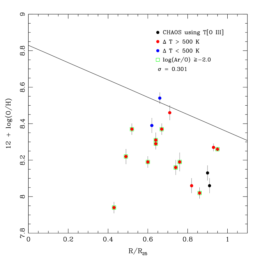
Figure 12.— The oxygen abundance gradient for NGC 628 using only [O III] for temperature determinations and the subsequent abundance analysis. The best least-squares fit determined in Section 4.3 is compared as a solid line, and the dispersion about this relationship is indicated. Regions used in the temperature discrepancy analysis are denoted as colored points, where the highly discrepant points are red and non-discrepant points are blue. Log(Ar/O) outliers are outlined by green boxes.

Appendix B INDICATORS OF TEMPERATURE DISCREPANCIES

[O III] has been and continues to be a useful temperature indicator, but significant deviations have emerged such that multiple cases must be considered, and the appropriate modifications applied: (1) In the case that T[O III]$\sim$T[S III], either indicator or an average may be adopted. (2) When T[S III]-T[O III] discrepancies are large, the multiple-line diagnostics presented throughout this paper indicate T[S III] should be used. (3) When T[O III] is the only measured temperature some risk of overestimating the temperature may be introduced, but in a systematic way such that oxygen abundance is underestimated.

In the last case of only one temperature determination, there is no potentially better alternative. However, if multiple auroral line detections are present, a further indication of how to proceed is needed. In this section we present two such indicators that appear promising as possible temperature diagnostics. We consider the standard choice of temperature indicators: T[O III] for the high ionization zone, T[S III] for the intermediate ionization zone, and T[N II] for the low ionization zone. The following plots are intended as an introduction for analysis to come with the completed CHAOS dataset, and so no conclusions are drawn here.

The ratio of [Ar III] $\lambda 7136$ to [S III] $\lambda 9069$ has been found to be insensitive to ionization structure, determined almost completely by the electron temperature and the ratio of the number of Ar and S ions (Stevenson et al., 1993), and therefore offers a more controlled look at temperature discrepancies. In Figure 13 we plot Ar⁺⁺/S⁺⁺ ratio versus the $\eta$ parameter (Vilchez & Pagel, 1988) for H II regions in NGC 628 . The $\eta$ parameter ($\eta$ = log[(O⁺/O⁺⁺)/(S⁺/S⁺⁺)]) represents the hardness of the input ionizing spectrum, and is a sensitive function of stellar effective temperature. This parameter pairing allows a more isolated temperature sensitive comparison and the implied result is striking. Most of the data follows a a linearly increasing relationship for log(Ar⁺⁺/S⁺⁺) vs log($\eta$), which is further confirmed by the non-discrepant T[S III]-T[O III] blue points that lie neatly along this trend. Further, most of the highly temperature discrepant red points are clear outliers. Some black points are also outliers, but they do not contain both temperature measurements required to assess temperature discrepancy. Based on this plot, Ar⁺⁺/S⁺⁺ is a useful diagnostic to identify extremely discrepant values of T[O III].

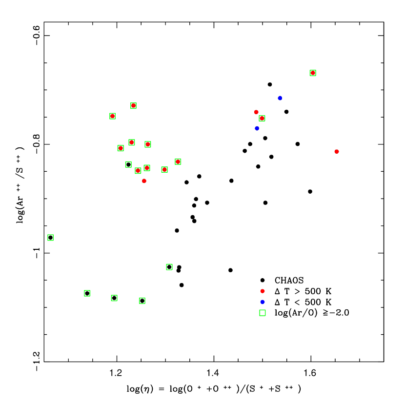
Figure 13.— Temperature sensitive indicators log(Ar⁺⁺/S⁺⁺) and log($\eta$) are plotted for NGC 628. Colored points are used to indicate regions where both T[S III] and T[O III] were measured, where highly discrepant regions are colored red and non-discrepant regions are blue. Regions with only one temperature measurement are colored black. Log(Ar/O) outliers are outlined by green boxes.

A second temperature discrepancy indicator of interest can be found in the $\alpha$-element abundance ratios. In general, $\alpha$-elements are thought to be produced primarily in massive stars and thus returned on similar time scales such that their ratio remains constant across oxygen abundance. However, Ar⁺⁺ and O⁺⁺ lie in different ionization zones, and so if large temperature discrepancies exist, we can expect to see regions with outlying values of log(Ar/O). Figure 14 demonstrates the usefulness of the Ar/O ratio as an indicator of temperature discrepancies. Log(Ar/O) is plotted versus oxygen abundance, using the standard choice of temperature indicators in the abundance analysis, and for the majority of the sample the anticipated constant trend is recovered, although the error-weighted average value is shifted up to log(Ar) $=-2.03$ and scatter is more than doubled ($\sigma_{t}=0.186$; $\sigma_{i}=0.172$). Above the dominant horizontal distribution of non-discrepant temperature points are a number of points with log(Ar/O) $\geq-2$, whose separation is denoted by a dotted line. Many of the Ar/O outliers, denoted by green boxes, correspond to large measured temperature discrepancies, and appear to be systematically offset to higher Ar/O ratios from the main sample. These outliers are consistent with the picture that overestimated [O III] temperatures produce underestimated oxygen abundances and thus overestimated Ar/O ratios. From these analyses, Ar has emerged as a possibly important gauge of temperature validity, and will be revisited in a more thorough analysis in a future paper.

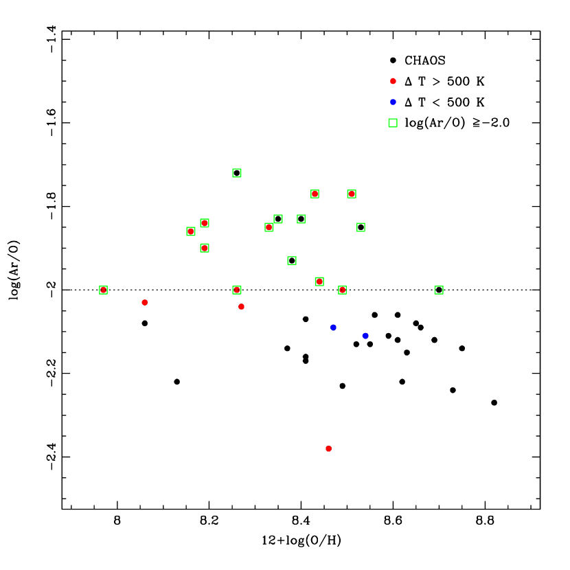
Figure 14.— The Ar/O ratio as a function of oxygen abundance is plotted for NGC628, where T[O III] is prioritized for the high ionization zone. The expected $\alpha$-element trend is recovered for the majority of the sample, but the resulting Ar/O values are higher on average (log(Ar/O) $=-2.033$) than the average value from our standard analysis (log(Ar/O) $=-2.219$; see Section 4.2) and the scatter greatly increased. A number of high Ar/O outliers (log(Ar/O) $\geq-2.0$; above dotted line) are present as indicated by green boxes. It is of interest that many of these outliers correspond to large discrepancies in T[S III]-T[O III].

References

- Allen et al. (2008) Allen, M. G., Groves, B. A., Dopita, M. A., Sutherland, R. S., & Kewley, L. J. 2008, ApJS, 178, 20
- Amorín et al. (2010) Amorín, R. O., Pérez-Montero, E., & Vílchez, J. M. 2010, ApJ, 715, L128
- Baldwin et al. (1981) Baldwin, J. A., Phillips, M. M., & Terlevich, R. 1981, PASP, 93, 5
- Berg et al. (2013) Berg, D. A., Skillman, E. D., Garnett, D. R., Croxall, K. V., Marble, A. R., Smith, J. D., Gordon, K., & Kennicutt, Jr., R. C. 2013, ApJ, 775, 128
- Berg et al. (2011) Berg, D. A., Skillman, E. D., & Marble, A. R. 2011, ApJ, 738, 2
- Berg et al. (2012) Berg, D. A., Skillman, E. D., Marble, A. R., et al. 2012, ApJ, 754, 98
- Binette et al. (2012) Binette, L., Matadamas, R., Hägele, G. F., et al. 2012, A&A, 547, A29
- Bohlin (2010) Bohlin, R. C. 2010, AJ, 139, 1515
- Bresolin (2007) Bresolin, F. 2007, ApJ, 656, 186
- Bresolin (2011) —. 2011, ApJ, 730, 129
- Bresolin et al. (2009a) Bresolin, F., Gieren, W., Kudritzki, R.-P., et al. 2009a, ApJ, 700, 309
- Bresolin et al. (1999) Bresolin, F., Kennicutt, R. C., J., & Garnett, D. R. 1999, ApJ, 510, 104
- Bresolin et al. (2005) Bresolin, F., Schaerer, D., González Delgado, R. M., & Stasińska, G. 2005, A&A, 441, 981
- Bruzual et al. (2013) Bruzual, G., Charlot, S., Lópezlira, R. G., et al. IAU Symposium, Vol. 295, , IAU Symposium, ed. D. ThomasA. Pasquali & I. Ferreras, 282–285
- Calzetti et al. (2000) Calzetti, D., Armus, L., Bohlin, R. C., et al. 2000, ApJ, 533, 682
- Castellanos et al. (2002) Castellanos, M., Díaz, A. I., & Terlevich, E. 2002, MNRAS, 329, 315
- Cedrés et al. (2012) Cedrés, B., Cepa, J., Bongiovanni, Á., et al. 2012, A&A, 545, A43
- Crockett et al. (2006) Crockett, N. R., Garnett, D. R., Massey, P., & Jacoby, G. 2006, ApJ, 637, 741
- Croxall et al. (2013) Croxall, K. V., Smith, J. D., Brandl, B. R., et al. 2013, ApJ, 777, 96
- Egusa et al. (2009) Egusa, F., Kohno, K., Sofue, Y., Nakanishi, H., & Komugi, S. 2009, ApJ, 697, 1870
- Esteban et al. (2009) Esteban, C., Bresolin, F., Peimbert, M., et al. 2009, ApJ, 700, 654
- Ferguson et al. (1998) Ferguson, A. M. N., Gallagher, J. S., & Wyse, R. F. G. 1998, AJ, 116, 673
- Fernandes et al. (2005) Fernandes, I. F., Gruenwald, R., & Viegas, S. M. 2005, MNRAS, 364, 674
- Filippenko (1982) Filippenko, A. V. 1982, PASP, 94, 715
- Froese Fischer & Tachiev (2004) Froese Fischer, C. & Tachiev, G. 2004, Atomic Data and Nuclear Data Tables, 87
- Froese Fischer et al. (2006) Froese Fischer, C., Tachiev, G., & Irimia, A. 2006, At. Data Nucl. Data Tables, 92, 607
- Garnett (1990) Garnett, D. R. 1990, ApJ, 363, 142
- Garnett (1992) Garnett, D. R. 1992, AJ, 103, 1330
- Gusev et al. (2012) Gusev, A. S., Pilyugin, L. S., Sakhibov, F., et al. 2012, MNRAS, 424, 1930
- Hägele et al. (2006) Hägele, G. F., Pérez-Montero, E., Díaz, Á. I., Terlevich, E., & Terlevich, R. 2006, MNRAS, 372, 293
- Hudson et al. (2012) Hudson, C. E., Ramsbottom, C. A., & Scott, M. P. 2012, ApJ, 750, 65
- Kauffman & Sugar (1986) Kauffman & Sugar. 1986, J. Phys. Chem. Ref. Data, 15, 339
- Kendall et al. (2011) Kendall, S., Kennicutt, R. C., & Clarke, C. 2011, MNRAS, 414, 538
- Kennicutt et al. (2011) Kennicutt, R. C., Calzetti, D., Aniano, G., et al. 2011, PASP, 123, 1347
- Kennicutt et al. (2003a) Kennicutt, Jr., R. C., Armus, L., Bendo, G., et al. 2003a, PASP, 115, 928
- Kennicutt et al. (2003b) Kennicutt, Jr., R. C., Bresolin, F., & Garnett, D. R. 2003b, ApJ, 591, 801
- Kennicutt & Hodge (1980) Kennicutt, Jr., R. C. & Hodge, P. W. 1980, ApJ, 241, 573
- Kewley et al. (2001) Kewley, L. J., Dopita, M. A., Sutherland, R. S., Heisler, C. A., & Trevena, J. 2001, ApJ, 556, 121
- Kewley & Ellison (2008) Kewley, L. J. & Ellison, S. L. 2008, ApJ, 681, 1183
- Kisielius et al. (2009) Kisielius, R., Storey, P. J., Ferland, G. J., & Keenan, F. P. 2009, MNRAS, 397, 903
- Lee & Skillman (2004) Lee, H. & Skillman, E. D. 2004, ApJ, 614, 698
- Lee et al. (2011) Lee, J. C., de Paz, G., A., K., R. C., J., et al. 2011, ApJS, 192, 6
- Markwardt (2009) Markwardt, C. B. Astronomical Society of the Pacific Conference Series, Vol. 411, , Astronomical Data Analysis Software and Systems XVIII, ed. D. A. BohlenderD. Durand & P. Dowler, 251
- McCall et al. (1985) McCall, M. L., Rybski, P. M., & Shields, G. A. 1985, ApJS, 57, 1
- McLaughlin & Bell (2000) McLaughlin, B. M. & Bell, K. L. 2000, J. Phys. B At. Mol. Phys., 33, 597
- Mendoza & Bautista (2014) Mendoza, C. & Bautista, M. A. 2014, ApJ, 785, 91
- Mendoza & Zeippen (1983) Mendoza, C. & Zeippen, C. J. 1983, MNRAS, 202, 981
- Moustakas et al. (2010) Moustakas, J., Kennicutt, R. C., J., Tremonti, C. A., et al. 2010, ApJS, 190, 233
- Muñoz-Mateos et al. (2009) Muñoz-Mateos, J. C., Gil de Paz, A., Zamorano, J., et al. 2009, ApJ, 703, 1569
- Munoz Burgos et al. (2009) Munoz Burgos, J. M., Loch, S. D., Ballance, C. P., & Boivin, R. F. 2009, A&A, 500, 1253
- Nava et al. (2006) Nava, A., Casebeer, D., Henry, R. B. C., & Jevremovic, D. 2006, ApJ, 645, 1076
- Nicholls et al. (2012) Nicholls, D. C., Dopita, M. A., & Sutherland, R. S. 2012, ApJ, 752, 148
- O’Donnell (1994) O’Donnell, J. E. 1994, ApJ, 422, 158
- Oke (1990) Oke, J. B. 1990, AJ, 99, 1621
- Peimbert (1967) Peimbert, M. 1967, ApJ, 150, 825
- Pérez-Montero & Díaz (2003) Pérez-Montero, E. & Díaz, A. I. 2003, MNRAS, 346, 105
- Pérez-Montero et al. (2006) Pérez-Montero, E., Díaz, A. I., Vílchez, J. M., & Kehrig, C. 2006, A&A, 449, 193
- Pilyugin (2005) Pilyugin, L. S. 2005, A&A, 436, L1
- Pilyugin et al. (2009) Pilyugin, L. S., Mattsson, L., Vílchez, J. M., & Cedrés, B. 2009, MNRAS, 398, 485
- Pogge et al. (2010) Pogge, R. W., Atwood, B., Brewer, D. F., Byard, P. L., Derwent, M. A., Gonzalez, R., Martini, P., Mason, J. A., O’Brien, T. P., Osmer, P. S., Pappalardo, D. P., Steinbrecher, D. P., Teiga, E. J., & Zhelem, R. 2010, in Society of Photo-Optical Instrumentation Engineers (SPIE) Conference Series, Vol. 7735, Society of Photo-Optical Instrumentation Engineers (SPIE) Conference Series
- Rosales-Ortega et al. (2011) Rosales-Ortega, F. F., Díaz, A. I., Kennicutt, R. C., & Sánchez, S. F. 2011, MNRAS, 415, 2439
- Rosolowsky & Simon (2008) Rosolowsky, E. & Simon, J. D. 2008, ApJ, 675, 1213
- Schlafly & Finkbeiner (2011) Schlafly, E. F. & Finkbeiner, D. P. 2011, ApJ, 737, 103
- Shostak & van der Kruit (1984) Shostak, G. S. & van der Kruit, P. C. 1984, A&A, 132, 20
- Skillman et al. (1994) Skillman, E. D., Televich, R. J., Kennicutt, Jr., R. C., Garnett, D. R., & Terlevich, E. 1994, ApJ, 431, 172
- Stasińska (1990) Stasińska, G. 1990, A&AS, 83, 501
- Stasińska (2010) Stasińska, G. in , IAU Symposium, Vol. 262, IAU Symposium, ed. G. R. BruzualS. Charlot, 93–96
- Stasińska et al. (2012) Stasińska, G., Prantzos, N., Meynet, G., et al., eds. 2012, EAS Publications Series, Vol. 54, Oxygen in the Universe
- Stevenson et al. (1993) Stevenson, C. C., McCall, M. L., & Welch, D. L. 1993, ApJ, 408, 460
- Storey et al. (2014) Storey, P. J., Sochi, T., & Badnell, N. R. 2014, MNRAS, 441, 3028
- Tachiev & Froese Fischer (2002) Tachiev, G. I. & Froese Fischer, C. 2002, A&A, 385, 716
- Talent (1983) Talent, D. L. 1983, PASP, 95, 986
- Tayal (2011) Tayal, S. S. 2011, ApJS, 195, 12
- Tayal & Gupta (1999) Tayal, S. S. & Gupta, G. P. 1999, ApJ, 526, 544
- Tayal & Zatsarinny (2010) Tayal, S. S. & Zatsarinny, O. 2010, ApJS, 188, 32
- Thuan et al. (1995) Thuan, T. X., Izotov, Y. I., & Lipovetsky, V. A. 1995, ApJ, 445, 108
- Tsamis et al. (2003) Tsamis, Y. G., Barlow, M. J., Liu, X.-W., Danziger, I. J., & Storey, P. J. 2003, MNRAS, 338, 687
- Tsamis et al. (2011) Tsamis, Y. G., Walsh, J. R., Vílchez, J. M., & Péquignot, D. 2011, MNRAS, 412, 1367
- Van Dyk et al. (2006) Van Dyk, S. D., Li, W., & Filippenko, A. V. 2006, PASP, 118, 351
- van Zee & Haynes (2006) van Zee, L. & Haynes, M. 2006, ApJ, 636, 214
- van Zee et al. (1998a) van Zee, L., Salzer, J. J., & Haynes, M. P. 1998a, ApJ, 497, L1
- van Zee et al. (1998b) van Zee, L., Salzer, J. J., Haynes, M. P., O’Donoghue, A. A., & Balonek, T. J. 1998b, AJ, 116, 2805
- Vilchez & Pagel (1988) Vilchez, J. M. & Pagel, B. E. J. 1988, MNRAS, 231, 257
- Weisz et al. (2015) Weisz, D. R., Johnson, L. C., Foreman-Mackey, D., Dolphin, A. E., Beerman, L. C., Williams, B. F., Dalcanton, J. J., Rix, H.-W., Hogg, D. W., Fouesneau, M., Johnson, B. D., Bell, E. F., Boyer, M. L., Gouliermis, D., Guhathakurta, P., Kalirai, J. S., Lewis, A. R., Seth, A. C., & Skillman, E. D. 2015, ArXiv e-prints
- Williams et al. (2010) Williams, M. J., Bureau, M., & Cappellari, M. 2010, MNRAS, 409, 1330
- Woosley & Weaver (1995) Woosley, S. E. & Weaver, T. A. 1995, ApJS, 101, 181
- Yin et al. (2007) Yin, S. Y., Liang, Y. C., Hammer, F., et al. 2007, A&A, 462, 535
- Zaritsky et al. (1994) Zaritsky, D., Kennicutt, J., C., R., & Huchra, J. P. 1994, ApJ, 420, 87
- Zurita & Bresolin (2012) Zurita, A. & Bresolin, F. 2012, MNRAS, 427, 1463