Nadav Drukker and Jan Felix
Department of Mathematics, King’s College London
The Strand, WC2R 2LS, London, UK

3d mirror symmetry as a canonical transformation

1 Introduction and summary

Supersymmetric localization leads to a dramatic simplification of the calculation of sphere partition functions (and some other observables) by reducing the infinite dimensional path integral to a finite dimensional matrix model [1, 2] This matrix model can then be solved (sometimes) by a variety of old and new techniques to yield exact results. A particular application of this is to check dualities — two theories which are equivalent (or flow to the same IR fixed point) should have the same partition function.

In practice, it is often very hard to solve the matrix models exactly, so dualities are checked by comparing the matrix models of the two theories and using integral identities to relate them. The first beautiful realization of this is in the Alday-Gaiotto-Tachikawa (AGT) correspondence, where the matrix models evaluating the partition functions of 4d ${\mathcal{N}}=2$ theories were shown to be essentially identical to correlation functions of Liouville theory as expressed via the conformal bootstrap in a specific channel. $S$-duality in 4d was then related to the associativity of the OPE in Liouville, which is manifested by complicated integral identities for the fusion and braiding matrices [3, 4, 5, 6, 7, 8].

Here we study 3d supersymmetric theories, which have several types of dualities, of which we will consider mirror symmetry and its $SL(2,\mathbb{Z})$ extension [9, 10, 11, 12, 13, 14]. Indeed one may use integral identities (in the simplest case just the Fourier transform of the sech function) [15] to show that the matrix models for certain mirror pairs are equivalent. But is there a way to simplify the calculation such that we can rely on a known duality of a model equivalent to the matrix model to get the answer without any work, as in the case of AGT?

Indeed for necklace quiver theories with at least ${\mathcal{N}}=3$ supersymmetry (and one copy of each bifundamental field) there is a simple realization of the matrix model in terms of a gas of non-interacting fermions in 1d with a complicated Hamiltonian [16]. The purpose of this note is to point out that the Hamiltonians of pairs of ${\mathcal{N}}=4$ mirror theories are related by a linear canonical transformation. Furthermore we show that the transformations between three known mirror theories close to $SL(2,\mathbb{Z})$, which is natural to identify with the $S$-duality group of type IIB, where the three theories have Hanany-Witten brane realizations.

In order to demonstrate this we generalize the Fermi-gas formalism of Mariño and Putrov to theories with nonzero Fayet-Iliopoulos (FI) parameters as well as mass terms for the bi-fundamental fields. This is presented in Section 2 where we focus for simplicity on a two-node circular quiver.

In section 3 we then present the action of mirror symmetry on the density operator of the Fermi-gas (the exponential of the Hamiltonian). We also outline the generalization to arbitrary circular quivers. The generalization of this formalism to $D$-quivers and theories with symplectic gauge group will be presented in [18].

In the appendix we proceed to evaluate the partition function of the two-node quiver (and its mirrors). This was done for the theory without FI terms and bifundamental masses in [16], and we here verify that the calculation can be carried through also with these parameters turned on. The resulting expressions are not modified much and one can still express them in terms of an Airy function.

2 Fermi-gas formalism with masses and FI-terms

In this section we review the Fermi-gas formulation [16] of the matrix model of 3d supersymmetric field theories and generalize it to a particular $\mathcal{N}=4$ theory that includes all of the ingredients we will require for our study of mirror symmetry in the following section. This is a two node quiver guage theory with gauge group $U(N)\times U(N)$. Each node has a Chern Simons (CS) term with levels $k$ and $-k$. There is a single matter hypermultiplet transforming in the fundamental representation of each $U(N)$ factor, and two matter hypermultiplets transforming in the bifundamental and anti-bifundamental representations of $U(N)\times U(N)$. The bifundamental fields have masses $m_{1}$ and $m_{2}$ and each node has a Fayet-Iliopoulos term with parameters $\zeta_{1}$ and $\zeta_{2}$.

The matrix model for this theory is computed via localisation [2]. The result can be easily derived by applying the rules presented for instance in [15, 19, 20]

$$Z(N)=\frac{1}{(N!)^{2}}\int d^{N}\lambda^{(1)}d^{N}\lambda^{(2)} \frac{\prod_{i<j}4\sinh^{2}\pi(\lambda^{(1)}_{i}-\lambda^{(1)}_{j})\,4\sinh^{2}\pi(\lambda^{(2)}_{i}-\lambda^{(2)}_{j})}{\prod_{i,j}2\cosh\pi(\lambda^{(1)}_{i}-\lambda^{(2)}_{j}+m_{1})\,2\cosh\pi(\lambda^{(2)}_{i}-\lambda_{j}^{(1)}+m_{2})}$$ (2.1)

$$\hskip 72.26999pt{}\times\prod_{i=1}^{N}\frac{e^{2\pi i\zeta_{1}\lambda^{(1)}_{i}+\pi ik(\lambda^{(1)}_{i})^{2}}e^{2\pi i\zeta_{2}\lambda^{(2)}_{i}-\pi ik(\lambda^{(2)}_{i})^{2}}}{2\cosh\pi{\lambda^{(1)}_{i}}\,2\cosh\pi{\lambda^{(2)}_{i}}}\,.$$

The crucial step in rewriting this expression as a Fermi-gas partition function is the use of the Cauchy determinant identity

$$\frac{\prod_{i<j}(x_{i}-x_{j})(y_{i}-y_{j})}{\prod_{i,j}(x_{i}-y_{j})}=\sum_{\sigma\in S_{N}}(-1)^{\sigma}\prod_{i=1}^{N}\frac{1}{(x_{i}-y_{\sigma(i)})}\,.$$ (2.2)

Applying this to (2.1) we may write the partition function as

$$Z(N)= \frac{1}{(N!)^{2}}\int d^{N}\lambda^{(1)}d^{N}\lambda^{(2)}\sum_{\sigma_{1}\in S_{N}}(-1)^{\sigma_{1}}\prod_{i=1}^{N}\frac{1}{2\cosh\pi(\lambda^{(1)}_{i}-\lambda^{(2)}_{\sigma_{1}(i)}+m_{1})}$$ (2.3)

$$\times\sum_{\sigma_{2}\in S_{N}}(-1)^{\sigma_{2}}\prod_{i=1}^{N}\frac{1}{2\cosh\pi(\lambda^{(2)}_{i}-\lambda^{(1)}_{\sigma_{2}(i)}+m_{2})}\prod_{i=1}^{N}\frac{e^{2\pi i\zeta_{1}\lambda^{(1)}_{i}+\pi ik(\lambda^{(1)}_{i})^{2}}e^{2\pi i\zeta_{2}\lambda^{(2)}_{i}-\pi ik(\lambda^{(2)}_{i})^{2}}}{2\cosh\pi{\lambda^{(1)}_{i}}2\cosh\pi{\lambda^{(2)}_{i}}}\,.$$

A relabelling of eigenvalues $\lambda^{(2)}_{i}\rightarrow\lambda^{(2)}_{\sigma^{\smash{-1}}_{1}(i)}$ allows us to resolve one of the sums over permutations, pulling out an overall factor of $N!$ giving

$$Z(N) =\frac{1}{N!}\sum_{\sigma\in S_{N}}(-1)^{\sigma}\int d^{N}\lambda^{(1)}_{i}\,d^{N}\lambda^{(2)}_{i}\prod_{i=1}^{N}\frac{e^{2\pi i\zeta_{1}\lambda^{(1)}_{i}}e^{i\pi k(\lambda^{(1)}_{i})^{2}}}{2\cosh\pi{\lambda^{(1)}_{i}}}\frac{1}{2\cosh\pi(\lambda^{(1)}_{i}-\lambda^{(2)}_{i}+m_{1})}$$ (2.4)

$$\hskip 144.54pt{}\times\frac{e^{2\pi i\zeta_{2}\lambda^{(2)}_{i}}e^{-i\pi k(\lambda^{(2)}_{i})^{2}}}{2\cosh\pi{\lambda^{(2)}_{i}}}\frac{1}{2\cosh\pi(\lambda^{(2)}_{i}-\lambda^{(1)}_{\sigma(i)}+m_{2})}$$

$$=\frac{1}{N!}\sum_{\sigma\in S_{N}}(-1)^{\sigma}\int d^{N}\lambda^{(1)}_{i}\,K\big{(}\lambda^{(1)}_{i},\lambda^{(1)}_{\sigma(i)}\big{)}.$$

Here we expressed the interaction between the eigenvalues $\lambda^{(1)}_{i}$ in terms of the kernel $K$, which can be considered the matrix element of the density operator $\hat{K}$ defined by

$$K(q_{1},q_{2})=\bra{q_{1}}\hat{K}\ket{q_{2}},\qquad\hat{K}=\frac{e^{2\pi i\zeta_{1}\hat{q}+\pi ik\hat{q}^{2}}}{2\cosh\pi\hat{q}}\,\frac{e^{2\pi im_{1}\hat{p}}}{2\cosh\pi\hat{p}}\,\frac{e^{2\pi i\zeta_{2}\hat{q}-\pi ik\hat{q}^{2}}}{2\cosh\pi\hat{q}}\,\frac{e^{2\pi im_{2}\hat{p}}}{2\cosh\pi\hat{p}}\,,$$ (2.5)

where $\hat{p}$ and $\hat{q}$ are canonical conjugate variables $[\hat{q},\hat{p}]=i\hbar$ with $\hbar=1/2\pi$ and we have made use of the elementary identities

$$f(\hat{q})\ket{q} =f(q)\ket{q}$$ (2.6)

$$e^{-2\pi im\hat{p}}f(\hat{q})e^{2\pi im\hat{p}} =f(\hat{q}-m)$$ (2.7)

$$\bra{q_{1}}\frac{1}{\cosh\pi\hat{p}}\ket{q_{2}} =\frac{1}{\cosh\pi(q_{1}-q_{2})}\,.$$ (2.8)

To study the system in a semiclassical expansion it is useful to represent the operators in Wigner’s phase space, where the Wigner transform of an operator $\hat{A}$ is defined as

$$A_{W}(q,p)=\int dq^{\prime}\Bra{q-\frac{q^{\prime}}{2}}\hat{A}\Ket{q+\frac{q^{\prime}}{2}}e^{ipq^{\prime}/\hbar}\,.$$ (2.9)

Some important properties are

$$(\hat{A}\hat{B})_{W}=A_{W}\star B_{W},\qquad\star=\exp\left[\frac{i\hbar}{2}\left(\overleftarrow{\partial_{q}}\overrightarrow{\partial_{p}}-\overrightarrow{\partial_{p}}\overleftarrow{\partial_{q}}\right)\right],\qquad\operatorname{Tr}(\hat{A})=\int\frac{dqdp}{2\pi\hbar}A_{W}\,.$$ (2.10)

For a detailed discussion of the phase space approach to Fermi-gasses see [16] and the original paper [21]. For a more general review of Wigner’s phase space and also many original papers see [22].

In the language of phase space the kernel $\hat{K}$ (2.5) becomes

$$K_{W}=\frac{e^{2\pi i\zeta_{1}q+\pi ikq^{2}}}{2\cosh\pi q}\star\frac{e^{2\pi im_{1}p}}{2\cosh\pi p}\star\frac{e^{2\pi i\zeta_{2}q-\pi ikq^{2}}}{2\cosh\pi q}\star\frac{e^{2\pi im_{2}p}}{2\cosh\pi p}\,.$$ (2.11)

Clearly the partition function can be determined from the spectrum of $\hat{K}$ or $K_{W}$. The leading classical part comes from replacing the star product with a regular product. In the appendix we outline the calculation of the partition function, extending [16].

3 Mirror symmetry

In this section we examine the theory studied in the previous section, with vanishing CS levels (see top quiver in Figure 1), where the density function (2.11) becomes

$$K_{W}=\frac{e^{2\pi i\zeta_{1}q}}{2\cosh\pi q}\star\frac{e^{2\pi im_{1}p}}{2\cosh\pi p}\star\frac{e^{2\pi i\zeta_{2}q}}{2\cosh\pi q}\star\frac{e^{2\pi im_{2}p}}{2\cosh\pi p}\,.$$ (3.1)

It has been known for a long time that this theory has two mirror theories, related in the IIB brane construction by $SL(2,\mathbb{Z})$ transformations [12]. As we show, the density functions of these theories are simply related by linear canonical transformations.

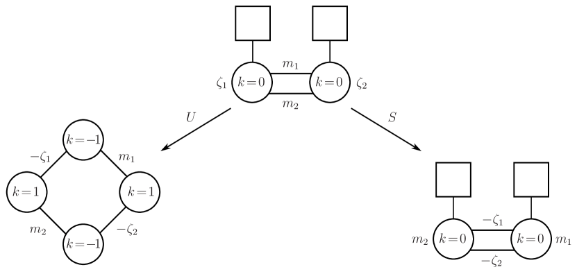
Figure 1: Quiver diagrams summarising the two node theory we discuss in the text and its two mirror duals. Each circle represents a $U(N)$ vector multiplet, labelled inside by the CS level $k$ and outside by the FI parameter. Edges represent hypermultiplets. Those connecting two circles are bifundamental fields with the mass indicated next to them. The boxes represent $U(1)$ flavor symmetries of fundamental hypers, which in our examples are massless.

3.1 $S$ transformation

The first of the known mirror theories is one with identical matter content but with mass and FI parameters exchanged [11]

$$m_{1}\rightarrow\tilde{m}_{1}=-\zeta_{1}\,,\qquad m_{2}\rightarrow\tilde{m}_{2}=-\zeta_{2}\,,\qquad\zeta_{1}\rightarrow\tilde{\zeta}_{1}=m_{2}\,,\qquad\zeta_{2}\rightarrow\tilde{\zeta}_{2}=m_{1}\,.$$ (3.2)

This is illustrated by the bottom right quiver in Figure 1.

At the level of the density function, this gives

$$K_{W}^{(S)}=\frac{e^{2\pi im_{2}q}}{2\cosh\pi q}\star\frac{e^{-2\pi i\zeta_{1}p}}{2\cosh\pi p}\star\frac{e^{2\pi im_{1}q}}{2\cosh\pi q}\star\frac{e^{-2\pi i\zeta_{2}p}}{2\cosh\pi p}\sim\frac{e^{-2\pi i\zeta_{1}p}}{2\cosh\pi p}\star\frac{e^{2\pi im_{1}q}}{2\cosh\pi q}\star\frac{e^{-2\pi i\zeta_{2}p}}{2\cosh\pi p}\star\frac{e^{2\pi im_{2}q}}{2\cosh\pi q}\,,$$ (3.3)

where the last relation represents equivalence under conjugating by $\frac{e^{2\pi im_{2}q}}{2\cosh\pi q}$. We find that this density is the same as (3.1) under the replacement

$$p\to q\,,\qquad q\to-p\,.$$ (3.4)

3.2 $U$ transformation

To get the second mirror theory we apply to (3.1) the replacement

$$p\rightarrow p+q\,,\qquad q\rightarrow-p\,.$$ (3.5)

The result is

$$K_{W}^{(U)} =\frac{e^{-2\pi i\zeta_{1}p}}{2\cosh\pi p}\star\frac{e^{2\pi im_{1}(p+q)}}{2\cosh\pi(p+q)}\star\frac{e^{-2\pi i\zeta_{2}p}}{2\cosh\pi p}\star\frac{e^{2\pi im_{2}(p+q)}}{2\cosh\pi(p+q)}$$ (3.6)

$$=\frac{e^{-2\pi i\zeta_{1}p}}{2\cosh\pi p}\star e^{-i\pi{q}^{2}}\star\frac{e^{2\pi im_{1}p}}{2\cosh\pi p}\star e^{i\pi{q}^{2}}\star\frac{e^{-2\pi i\zeta_{2}p}}{2\cosh\pi p}\star e^{-i\pi{q}^{2}}\star\frac{e^{2\pi im_{2}p}}{2\cosh\pi p}\star e^{i\pi{q}^{2}}\,.$$

In the second line we have made use of the identity

$$e^{-\pi i{q}^{2}}\star f(p)\star e^{\pi i{q}^{2}}=f(p+q)\,.$$ (3.7)

To read off the corresponding quiver theory from (3.6), each $e^{i\pi(kq^{2}+2\zeta q)}$ term can be associated to a $U(N)$ node with CS level $k$ and FI parameter $\zeta$, while each $\frac{e^{2\pi imp}}{2\cosh\pi p}$ comes from a bifundamental hypermultiplet with mass $m$. The transformed density operator corresponds therefore to a circular quiver with four nodes that have alternating Chern-Simons levels $k=\pm 1$ and vanishing FI parameters. The bifundamental multiplets connecting adjacent nodes have masses $\{-\zeta_{1},m_{1},-\zeta_{2},m_{2}\}$, as in the bottom left diagram of Figure 1.

As we discuss in the appendix, the partition function can be expressed in terms of $\operatorname{Tr}\hat{K}^{l}$ (A.1), which in phase space is given by an integral over $p,q$ (2.10). Since we showed that mirror symmetry can be viewed just as a linear canonical transformation, which is a change of variables with unit Jacobian, it is clear that mirror symmetry preserves the partition function.

3.3 $SL(2,\mathbb{Z})$

It is easy to see that the transformations we used in the previous sections close onto $SL(2,\mathbb{Z})$. Indeed, defining $T=SU$ we find the defining relations

$$S^{2}=-I\,,\qquad(ST)^{3}=I\,.$$ (3.8)

More general $SL(2,\mathbb{Z})$ transformations will give density operators with terms of the form

$$\frac{1}{\cosh\pi(ap+bq)}\,.$$ (3.9)

The cases with $a=0$ and $b=1$ or $a=\pm 1$ and $b\in\mathbb{Z}$ have a natural interpretation as a contribution of a fundamental field, or as we have seen in (3.7), from conjugating the usual $1/\cosh\pi p$ by CS terms. But these manipulations cannot undo expressions one finds from a general $SL(2,\mathbb{Z})$ transformation of $K_{W}$. In these more general cases, the transformed density operator can still be associated to a matrix model, but it cannot be derived from any known 3d lagrangian.

This is also manifested in the IIB brane realization, where any $SL(2,\mathbb{Z})$ transformation will lead to some configuration of $(p,q)$ branes. Most of those do not have a known Lagrangian description [23], but one could associate to them a matrix model [14], which would indeed lead to the transformed density operator.

3.4 Mirror symmetry for generic circular quiver

The manifestation of mirror symmetry as a canonical transformation naturally generalises to the entire family of ${\mathcal{N}}=4$ circular quivers with an arbitrary number of nodes. Applying the Fermi-gas formalism, it is easy to see that the density function for such a theory with $n$ nodes is given by

$$K_{W}=\prod_{a=1}^{n}\raisebox{-5.16663pt}{}_{\star}\frac{e^{2\pi i\zeta_{a}q}}{\left(2\cosh\pi q\right)^{N_{a}}}\star\frac{e^{2\pi im_{a}p}}{2\cosh\pi p}\,,$$ (3.10)

where $\zeta_{a}$ denotes the FI parameter of the $a$^th node, $N_{a}$ denotes the number of fundamental matter fields attached to the $a$^th node and $m_{a}$ denotes the mass of the bifundamental field connecting the $a$^th and $(a+1)$^th nodes.

We can now apply the $S$ and $U$ transformations of the previous section, and look to see if the resulting density functions can again be interpreted as coming from the mirror gauge theories. Applying the $S$ transformation we get

$$K_{W}^{(S)}=\prod_{a=1}^{n}\raisebox{-5.16663pt}{}_{\star}\frac{e^{-2\pi i\zeta_{a}p}}{\left(2\cosh\pi p\right)^{N_{a}}}\star\frac{e^{2\pi im_{a}q}}{2\cosh\pi q}\,.$$ (3.11)

This density function is that of a circular quiver theory with $\sum_{a=1}^{n}N_{a}$ nodes and $n$ fundamental matter fields. The fundamentals are attached to nodes which have FI parameters $m_{a}$, and are separated by $N_{a}-1$ other nodes. The masses of the bifundamentals connecting them add up to $-\zeta_{a}$.

Applying the $U$ transformation we get

$$K_{W}^{(U)}=\prod_{a=1}^{n}\raisebox{-5.16663pt}{}_{\star}\frac{e^{-2\pi i\zeta_{a}p}}{\left(2\cosh\pi p\right)^{N_{a}}}\star\frac{e^{2\pi im_{a}(p+q)}}{2\cosh\pi(p+q)}=\prod_{a=1}^{n}\raisebox{-5.16663pt}{}_{\star}\frac{e^{-2\pi i\zeta_{a}p}}{\left(2\cosh\pi p\right)^{N_{a}}}\star e^{-\pi iq^{2}}\star\frac{e^{2\pi im_{a}p}}{2\cosh\pi p}\star e^{\pi iq^{2}}\,.$$ (3.12)

The mirror theory can be readily read off from this density function as a circular quiver theory with $\sum_{a=1}^{n}N_{a}+n$ nodes and no fundamental matter. Each node has Chern-Simons level $k=+1,-1$ or $0$. Further details concerning the mass parameters and value of the Chern-Simons level at each node can be read off in much the same way as for the previous example.

A further generalisation we have not yet considered is to turn on masses for the fundamental fields. This corresponds to replacing each of the $(2\cosh\pi q)^{-N_{a}}$ in (3.10) with a product of $N_{a}$ terms with masses $\mu_{i}$

$$e^{2\pi i\zeta_{a}q}\star\prod_{i=1}^{N_{a}}\raisebox{-5.16663pt}{}_{\star}\frac{1}{2\cosh\pi(q+\mu_{i})} =e^{2\pi i\zeta_{a}q}\star\prod_{i=1}^{N_{a}}\raisebox{-5.16663pt}{}_{\star}\left(e^{2\pi i\mu_{i}p}\star\frac{1}{2\cosh\pi q}\star e^{-2\pi i\mu_{i}p}\right)$$ (3.13)

$$\hskip-86.72377pt{}=e^{-2\pi i\zeta_{a}\mu_{1}}e^{2\pi i\mu_{1}p}\star\frac{e^{2\pi i\zeta_{a}q}}{2\cosh\pi q}\star e^{-2\pi i\mu_{1}p}\star\prod_{i=2}^{N_{a}}\raisebox{-5.16663pt}{}_{\star}\left(e^{2\pi i\mu_{i}p}\star\frac{1}{2\cosh\pi q}\star e^{-2\pi i\mu_{i}p}\right).$$

Where in the second line we chose to associate the FI term to the first fundamental field, picking up an overall phase.

Once we apply $S$ or $U$ transformations to (3.13) it becomes clear that these mass terms become additional FI parameters, as is expected.

Acknowlegments

We are grateful to Benjamin Assel and Marcos Mariño for useful discussions. N.D. is grateful for the hospitality of APCTP, of Nordita, CERN (via the CERN-Korea Theory Collaboration) and the Simons Center for Geometry and Physics, Stony Brook University during the course of this work. The research of N.D. is underwritten by an STFC advanced fellowship. The CERN visit was funded by the National Research Foundation (Korea). The research of J.F. is funded by an STFC studentship ST/K502066/1

Appendix A From density to Airy function

In this appendix we outline the computation of the large $N$ partition function for a theory with mass and FI parameters. Since the calculation follows closely the method outlined in [16] we will be rather cursory and refer the reader to [16] for more detail, highlighting the new features that appear due to the FI and mass parameters.

To evaluate (2.4), one notices that it combines to give products of $Z_{l}=\operatorname{Tr}(K_{W})^{l}$ where the values of $l$ depends only on the conjugacy class of $\sigma$. Instead of summing over all permutations we can sum over conjugacy classes which have $m_{l}$ cycles of length $l$ and the combinatorics give

$$Z(N)={\sum_{\{m_{l}\}}}^{\prime}\prod_{l}\frac{(-1)^{(l-1)m_{l}}Z_{l}^{m_{l}}}{m_{l}!l^{m_{l}}}\,,$$ (A.1)

where the primed sum denotes the restriction to sets that satisfy $\sum_{l}lm_{l}=N$. Following the usual analysis from statistical mechanics [24] we consider the grand canonical partition function given by

$$\Xi(\mu)=1+\sum_{N=1}^{\infty}Z(N)e^{\mu N}=\text{Exp}\left[-\sum_{l=1}^{\infty}\frac{(-1)^{l}Z_{l}e^{\mu l}}{l}\right].$$ (A.2)

We consider the density function (3.1), and using (2.7), (2.10) rewrite it as

$$K_{W} =e^{\pi i(m_{1}\zeta_{2}-\frac{1}{2}\zeta_{1}m_{1}-\frac{1}{2}\zeta_{2}m_{2})}e^{\pi i((2\zeta_{1}+\zeta_{2})q+m_{1}p)}\star\frac{1}{2\cosh\pi(q-\frac{m_{1}}{2})}\star\frac{1}{2\cosh\pi(p+\frac{\zeta_{2}}{2})}$$ (A.3)

$$\hskip 112.0187pt{}\star\frac{1}{2\cosh\pi(q+\frac{m_{1}}{2})}\star\frac{1}{2\cosh\pi(p-\frac{\zeta_{2}}{2})}\star e^{\pi i(\zeta_{2}q+(m_{1}+2m_{2})p)}\,.$$

In order to get a hermetian Hamiltonian below, we specialize to the case

$$\zeta_{1}=-\zeta_{2}=\zeta\,,\qquad m_{1}=-m_{2}=m\,,$$ (A.4)

and conjugate

$$K_{W}\rightarrow(2\cosh\pi(q-\tfrac{m}{2}))^{\frac{1}{2}}\star e^{-\pi i(mp+\zeta q)}\star K_{W}\star e^{\pi i(\zeta q+mp)}\star\frac{1}{(2\cosh\pi(q-\frac{m}{2}))^{\frac{1}{2}}}\,.$$ (A.5)

This gives the kernel

$${K_{W}}=\frac{e^{-2\pi i\zeta m}}{(2\cosh\pi(q-\frac{m}{2}))^{\frac{1}{2}}}\star\frac{1}{2\cosh\pi(p-\frac{\zeta}{2})}\star\frac{1}{2\cosh\pi(q+\frac{m}{2})}\star\frac{1}{2\cosh\pi(p+\frac{\zeta}{2})}\star\frac{1}{(2\cosh\pi(q-\frac{m}{2}))^{\frac{1}{2}}}\,.$$ (A.6)

The phase in $K_{W}$ leads to an overall phase $(e^{-2\pi i\zeta m})^{N}$ in front of the partition function and can be removed and reintroduced at the end (A.19).

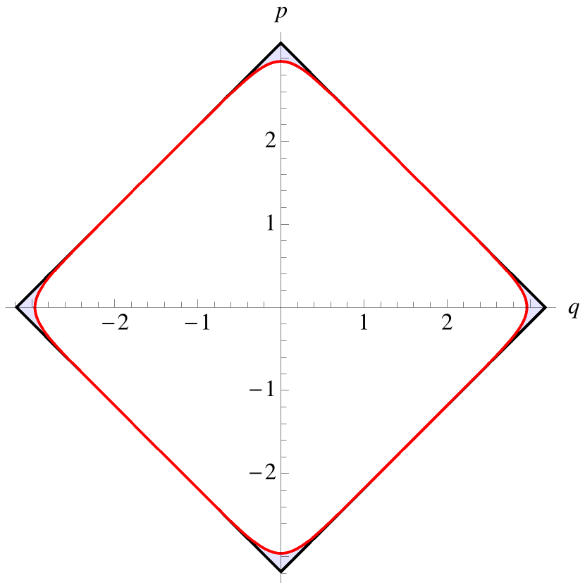
(a)    

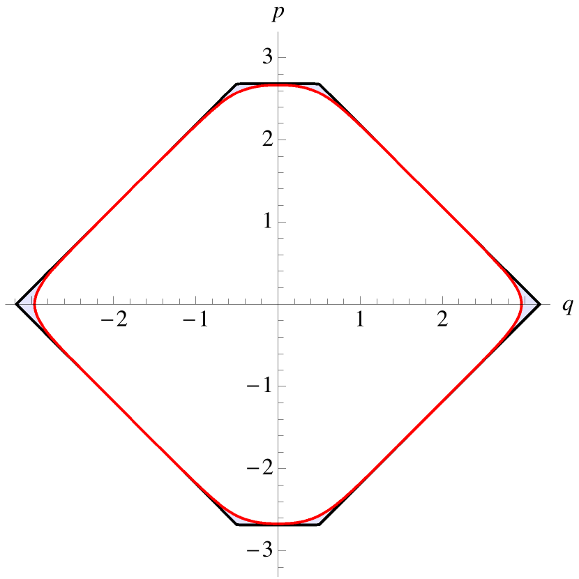
(b)    

Figure 2: Fermi surfaces for $E=20$ and masses $m=0$ (a) and $m=1$ (b). The red lines are the exact classical Hamiltonians (A.8) and black lines the polygon approximation (A.9). The region between them is the leading order perturbative correction given in the first line of (A.13).

Following Section 4 of [16] we compute the partition function by studying the spectrum of the one particle Hamiltonian

$$H_{W}=-\log_{*}K_{W}\,.$$ (A.7)

To find an expression for $H_{W}$ one must perform a Baker-Campbell-Hausdorff (BCH) expansion of the logarithm in (A.7). Setting $\zeta=0$, the leading classical term in this expansion is simply

$$H_{\text{cl}}=\log\left(2\cosh\pi\left(q+\frac{m}{2}\right)\right)+\log\left(2\cosh\pi\left(q-\frac{m}{2}\right)\right)+2\log(2\cosh\pi p)\,.$$ (A.8)

For large $p,q$ this is

$$H_{\text{cl}}\approx\pi\left|q+\frac{m}{2}\right|+\pi\left|q-\frac{m}{2}\right|+2\pi|p|\,.$$ (A.9)

It is clear that the approximate Hamiltonian is independent of $m$ for $\left|q\right|>\frac{m}{2}$. In Figure 2 we display the exact classical Fermi surface and polygonal approximation for a particular value of $E$ and with vanishing and non vanishing mass. The only change to the polygon from turning on the mass is the removal of the two triangles with $|p|>\frac{E}{2\pi}-\frac{m}{2}$ whose combined area is $m^{2}/2$.

The number of states below the energy $E$ is given by the area enclosed by the curve $H=E$. Using the polynomial approximation this is just

$$n(E)\approx\int dqdp\,\theta\!\left(E-\pi\left|q-\frac{m}{2}\right|-\pi\left|q-\frac{m}{2}\right|-2\pi|p|\right)=CE^{2}-\frac{m^{2}}{2},\qquad C=\frac{1}{2\pi^{2}}\,.$$ (A.10)

This expression is only approximate and gets corrected by accounting for the difference between (A.9) and the exact quantum Hamiltonian (A.7). We do this by modifying the number of states to

$$n(E)=CE^{2}-\frac{m^{2}}{2}+n_{0}+n_{\text{np}}(E)\,,$$ (A.11)

We outline the calculation of $n_{0}$ below. The main point is that it does not depend on $m$. $n_{\text{np}}$ denote nonperturbative, exponentially suppressed corrections at large $E$, but are such that $n(0)=0$. To satisfy this, $n_{\text{np}}$ clearly has to depend on $m$, but this will have no effect on our end result where we ignore the nonperturbative terms. The approximation (A.9) is valid where both $p$ or $q$ are large, and as shown in [16], the quantum corrections to (A.8) (from the BCH expansion of (A.7)) are also exponentially suppressed there. All the corrections are therefore associated with regions where either $p$ or $q$ are small, namely around the vertices of the polygon. We then consider the contributions to $n_{0}$ from each region separately, integrating in each case the (perturbative) corrections to the boundary. For instance, around $q\sim 0$, $p\gg 1$ the first quantum corrections of the Hamiltonian are given (up to terms exponentially suppressed in $p$) by

$$H_{\text{cl}}\to H_{\text{cl}}+\frac{\pi^{2}}{24}\left(\frac{1}{\cosh^{2}\pi(q+\frac{m}{2})}-\frac{2}{\cosh^{2}\pi(q-\frac{m}{2})}\right)\,.$$ (A.12)

The difference in the area between the polygon and the quantum corrected Fermi surface for large $E$ approaches

$$\int_{-\infty}^{\infty}\frac{dq}{2\pi}\Bigg{[} \pi\left|q+\frac{m}{2}\right|+\pi\left|q-\frac{m}{2}\right|-\log 2\cosh\pi\left(q+\frac{m}{2}\right)-\log 2\cosh\pi\left(q-\frac{m}{2}\right)$$ (A.13)

$${}-\frac{\pi^{2}}{24}\left(\frac{1}{\cosh^{2}\pi(q+\frac{m}{2})}-\frac{2}{\cosh^{2}\pi(q-\frac{m}{2})}\right)\Bigg{]}=-\frac{1}{24}\,.$$

As advertised, this is independent of $m$ (which can be seen by splitting the integral into two term with $q\pm m/2$ and shifting the integration variable).

The analog expression around the $p=0$, $q\gg 1$ vertex is

$$\int_{-\infty}^{\infty}\frac{dp}{2\pi}\left(2\pi|p|-2\log 2\cosh\pi p-\frac{\pi^{2}}{48\cosh^{2}\pi p}\right)=-\frac{5}{48}\,.$$ (A.14)

Summing over the contributions from all four regions we get

$$n_{0}=2\left(-\frac{1}{24}-\frac{5}{48}\right)=-\frac{7}{24}\,.$$ (A.15)

It is not hard to see that all the higher order quantum corrections do not modify $n_{0}$ and in particular do not depend on $m$. See the discussion in Section 5.3 of [16].

From $n(E)$ it is easy to calculate the matrix model partition function. The grand canonical potential, the logarithm of (A.2) is

$$J(\mu)=\log\Xi(\mu)=\int_{0}^{\infty}dE\rho(E)\log(1+e^{\mu-E})\,,\qquad\rho(E)=\frac{dn(E)}{dE}\,.$$ (A.16)

At large $\mu$ this integral reduces to

$$J(\mu)=\frac{C}{3}\mu^{3}+\mu\left(n_{0}-\frac{m^{2}}{2}+\frac{\pi^{2}C}{3}\right)+A+\mathcal{O}(\mu e^{-\mu})\,.$$ (A.17)

$A$ is a constant that we will not concern ourselves with (it is studied in more detail in [16] and subsequent papers). From this we can extract the canonical partition function

$$Z(N)=\frac{1}{2\pi i}\int_{-i\infty}^{i\infty}e^{J(\mu)-\mu N}=C^{-\frac{1}{3}}e^{A}\operatorname{Ai}\left[C^{-\frac{1}{3}}\left(N-n_{0}-\frac{\pi^{2}C}{3}+\frac{m^{2}}{2}\right)\right]+{\mathcal{O}}(e^{-N})\,.$$ (A.18)

It is straight forward to include also the FI parameter $\zeta$. Remembering the extra phase in (A.6) one finds

$$Z(N)=C^{-\frac{1}{3}}e^{A-2\pi i\zeta mN}\operatorname{Ai}\left[C^{-\frac{1}{3}}\left(N-n_{0}-\frac{\pi^{2}C}{3}+\frac{m^{2}+\zeta^{2}}{2}\right)\right].$$ (A.19)

One can treat quite general $\mathcal{N}=3$ necklace quiver theories in a similar fashion, subject to the technical constraint that the sum over FI parameters and the sum over bifundamental masses both vanish. The analog of (A.9) will again be a piecewise linear Hamiltonian

$$H\approx\sum_{i}|a_{i}q+b_{i}p+c_{i}|\,,$$ (A.20)

The parameters $a_{i}$ and $b_{i}$ are determined by the Chern-Simons terms and $c_{i}$ are due to mass and FI terms. The volume of the corresponding polygonal Fermi surface is again of the form

$$CE^{2}+B$$ (A.21)

Similar arguments to those made above guarantee that the full $c_{i}$ dependence appears via a shift $B$ which can be found already in the polygonal approximation.

References

- [1] V. Pestun, “Localization of gauge theory on a four-sphere and supersymmetric Wilson loops,” Commun.Math.Phys. 313 (2012) 71–129, arXiv:0712.2824.
- [2] A. Kapustin, B. Willett, and I. Yaakov, “Exact results for Wilson loops in superconformal Chern-Simons theories with matter,” JHEP 1003 (2010) 089, arXiv:0909.4559.
- [3] L. F. Alday, D. Gaiotto, and Y. Tachikawa, “Liouville correlation functions from four-dimensional gauge theories,” Lett.Math.Phys. 91 (2010) 167–197, arXiv:0906.3219.
- [4] H. Dorn and H. Otto, “Two and three point functions in Liouville theory,” Nucl.Phys. B429 (1994) 375–388, hep-th/9403141.
- [5] A. B. Zamolodchikov and A. B. Zamolodchikov, “Structure constants and conformal bootstrap in Liouville field theory,” Nucl.Phys. B477 (1996) 577–605, hep-th/9506136.
- [6] B. Ponsot and J. Teschner, “Liouville bootstrap via harmonic analysis on a noncompact quantum group,” hep-th/9911110.
- [7] J. Teschner, “Liouville theory revisited,” Class.Quant.Grav. 18 (2001) R153–R222, hep-th/0104158.
- [8] N. A. Nekrasov, “Seiberg-Witten prepotential from instanton counting,” Adv.Theor.Math.Phys. 7 (2004) 831–864, hep-th/0206161.
- [9] K. A. Intriligator and N. Seiberg, “Mirror symmetry in three-dimensional gauge theories,” Phys.Lett. B387 (1996) 513–519, hep-th/9607207.
- [10] A. Hanany and E. Witten, “Type IIB superstrings, BPS monopoles, and three-dimensional gauge dynamics,” Nucl.Phys. B492 (1997) 152–190, hep-th/9611230.
- [11] J. de Boer, K. Hori, H. Ooguri, and Y. Oz, “Mirror symmetry in three-dimensional gauge theories, quivers and D-branes,” Nucl.Phys. B493 (1997) 101–147, hep-th/9611063.
- [12] J. de Boer, K. Hori, H. Ooguri, Y. Oz, and Z. Yin, “Mirror symmetry in three-dimensional theories, and D-brane moduli spaces,” Nucl.Phys. B493 (1997) 148–176, hep-th/9612131.
- [13] E. Witten, “SL(2,Z) action on three-dimensional conformal field theories with Abelian symmetry,” hep-th/0307041.
- [14] B. Assel, “Hanany-Witten effect and dualities in matrix models,” arXiv:1406.5194.
- [15] A. Kapustin, B. Willett, and I. Yaakov, “Nonperturbative tests of three-dimensional dualities,” JHEP 1010 (2010) 013, arXiv:1003.5694.
- [16] M. Mariño and P. Putrov, “ABJM theory as a Fermi gas,” J.Stat.Mech. 1203 (2012) P03001, arXiv:1110.4066.
- [17] T. Dimofte, D. Gaiotto, and S. Gukov, “Gauge theories labelled by three-manifolds,” Commun.Math.Phys. 325 (2014) 367–419, arXiv:1108.4389.
- [18] B. Assel, N. Drukker, and J. Felix, in preparation.
- [19] D. R. Gulotta, C. P. Herzog, and T. Nishioka, “The ABCDEF’s of matrix models for supersymmetric Chern-Simons theories,” JHEP 1204 (2012) 138, arXiv:1201.6360.
- [20] I. Yaakov, “Localization of gauge theories on the three-sphere,”. http://thesis.library.caltech.edu/7116/1/Thesis_Itamar_Yaakov_2012.pdf.
- [21] B. Grammaticos and A. Voros, “Semiclassical approximations for nuclear Hamiltonians. 1. spin independent potentials,” Annals Phys. 123 (1979) 359.
- [22] C. Zachos, D. Fairlie, and T. Curtright, Quantum mechanics in phase space: an overview with selected papers. World Scientific Publishing Company, 2005.
- [23] D. Gaiotto and E. Witten, “-Duality of boundary conditions in super Yang-Mills theory,” Adv.Theor.Math.Phys. 13 (2009) 721, arXiv:0807.3720.
- [24] R. Feynman, Statistical mechanics: a set of lectures. 1972.
- [25] Y. Hatsuda, S. Moriyama, and K. Okuyama, “Instanton effects in ABJM theory from Fermi gas approach,” JHEP 1301 (2013) 158, arXiv:1211.1251.