Abstract

Within the Constrained Minimal Supersymmetric Standard Model (CMSSM) with Minimal Flavor Violation (MFV) for scalar quarks we study the effects of intergenerational squark mixing on $B$-physics observables, electroweak precision observables (EWPO) and the Higgs boson mass predictions. Squark mixing is generated through the Renormalization Group Equations (RGE) running from the GUT scale to the electroweak scale due to presence of non diagonal Yukawa matrices in the RGE’s, e.g. due to the CKM matrix. We find that the $B$-Physics observables as well as the Higgs mass predictions do not receive sizable corrections. On the other hand, the EWPO such as the $W$ boson mass can receive corrections by far exceeding the current experimental precision. These contributions can place new upper bounds on the CMSSM parameter space. We extend our analysis to the CMSSM extended with a mechanism to explain neutrino masses (CMSSM-seesaw I), which induces flavor violation in the scalar lepton sector. Effects from slepton mixing on the analyzed observables are in general smaller than from squark mixing, but can reach the level of the current experimenal uncertainty for the EWPO.

1 Introduction

Supersymmetric (SUSY) extensions of the Standard Model (SM) are broadly considered as the most motivated and promising New Physics (NP) theories beyond the SM. The solution of the hierarchy problem, the gauge coupling unification and the possibility of having a natural cold dark matter candidate, constitute the most convincing arguments in favor of SUSY.

Within the Minimal Supersymmetric Standard Model (MSSM) [1], flavor mixing can occur in both scalar quark and scalar lepton sector. Here the possible presence of soft SUSY-breaking parameters in the squark and slepton sector, which are off-diagonal in flavor space (mass parameters as well as trilinear couplings) are the most general way to introduce flavor mixing within the MSSM. This, however, yields many new sources of flavor and ${\cal CP}$-violation, which potentially lead to large non-standard effects in flavor processes in conflict with experimental bounds.

The SM has been very successfully tested by low-energy flavor observables both from the kaon and $B_{d}$ sectors. In particular, the two $B$ factories have established that $B_{d}$ flavor and ${\cal CP}$-violating processes are well described by the SM up to an accuracy of the $\sim 10\%$ level [2]. This immediately implies a tension between the solution of the hierarchy problem, calling for a NP scale at or below the TeV scale, and the explanation of the Flavor Physics data requiring a multi-TeV NP scale if the new flavor-violating couplings are of generic size.

An elegant way to simultaneously solve the above problems is provided by the Minimal Flavor Violation (MFV) hypothesis [3, 4], where flavor and ${\cal CP}$-violation in quark sector are assumed to be entirely described by the CKM matrix. Even in theories beyond the SM. For example in MSSM, the off-diagonality in the sfermion mass matrix reflects the misalignment (in flavor space) between fermions and sfermions mass matrices, that cannot be diagonalized simultaneously. This misalignment can be produced from various origins. For instance, off-diagonal sfermion mass matrix entries can be generated by Renormalization Group Equations (RGE) running. Going from a high energy scale, where no flavor violation is assumed, down to the electroweak (EW) scale can generate such entries due to presence of non diagonal Yukawa matrices in RGE’s. For example, in the Constrained Minimal Supersymmetric Standard Model (CMSSM, see Ref. [5] and references therein), the left-handed scalar-quark soft SUSY-breaking parameter RGE’s have a general form:

$$\frac{d}{dt}(m_{\tilde{Q}}^{2})_{ij}\propto a{\rm 1\kern-1.19995pt\rule{0.3pt}{6.45831pt}\raisebox{0.0pt}{\rule{1.00006pt}{0.3pt}}}_{ij}+b(Y_{U}^{{\dagger}}Y_{U})_{ij}$$ (1)

where $a$ and $b$ are some constants, the up-quark Yukawa matrix, $Y_{U}$, is non-diagonal, and $t=\log\frac{\mu}{\mu_{0}}$ with $\mu\,(\mu_{0})$ is the running (fixed) scale.

It is convenient to work in the basis in which the Yukawa couplings are given by

$$Y_{D}={\rm diag}(y_{d},y_{s},y_{b}),\quad Y_{U}=V_{\rm CKM}^{{\dagger}}{\rm diag}(y_{u},y_{c},y_{t})$$ (2)

and hence all flavor violation in the quark and squark sector is controlled by the CKM matrix.

The situation is somewhat different in the slepton sector where neutrinos are strictly massless (in the SM and the MSSM) Consequently, there is no slepton mixing, which would induce Lepton Flavor Violation (LFV) in the charged sector, allowing not yet observed processes like $l_{i}\to l_{j}\gamma$ ($i>j$; $l_{3,2,1}=\tau,\mu,e$) [6]. However in the neutral sector, we have strong experimental evidence that shows that the neutrinos are massive and mix among themselves [7]. In order to incorporate this one needs to go beyond the MSSM to introduce a mechanism that generates neutrino masses. The simplest way would be to introduce Dirac masses, however, leaving the extreme smallness of the neutrino masses unexplained. To overcome this problem, typically a see-saw mechanism is used to generate neutrino masses, and the PMNS matrix plays the role of the CKM matrix in the lepton sector. Extending the MFV hypothesis for leptons [8] we can assume that the flavor mixing in the lepton and slepton sector is induced and controlled by the see-saw mechanism.

Consequently, in this paper we will investigate two models (more detailed definitions are given in the next section):

• the CMSSM, where only flavor violation in the squark sector is present.

• the CMSSM augmented by the seesaw type I mechanism[9], called “CMSSM-seesaw I” below.

In many analyses of the CMSSM, or extensions such as the NUHM1 or NUHM2 (see Ref. [5] and references therein), the hypothesis of MFV has been used, and it has been assumed that the contributions coming from MFV are negligible for other observables as well, see, e.g., Ref. [10]. In this paper we will analyze whether this assumption is justified, and whether including these MFV effects could lead to additional constraints on the CMSSM parameter space. In this respect we evaluate in the CMSSM and in the CMSSM-seesaw I the following set of observables: $B$ physics observables (BPO), in particular ${\rm BR}(B\to X_{s}\gamma)$, ${\rm BR}(B_{s}\to\mu^{+}\mu^{-})$ and $\Delta M_{B_{s}}$, electroweak precision observables (EWPO), in particular $M_{W}$ and the effective weak leptonic mixing angle, $\sin^{2}\theta_{\mathrm{eff}}$, as well as the masses of the neutral and charged Higgs bosons in the MSSM.

In order to perform our calculations, we used SPheno [11] to generate the CMSSM (containing also the type I seesaw) particle spectrum by running RGE from the GUT down to the EW scale. The particle spectrum was handed over in the form of an SLHA file [12] to FeynHiggs [13, 14, 15, 16, 17] to calculate EWPO and Higgs boson masses. The $B$-Physics observables were calculated by the BPHYSICS subroutine included in the SuFla code [18] (see also Refs. [19, 20] for the improved version used here).

The paper is organized as follows: First we review the main features of the MSSM with sfermion flavor mixing in MFV in Sect. 2. The computational setup is given in Sect. 3. The numerical results are presented in Sect. 4, where first we discuss the effect of squarks mixing in the CMSSM. In a second step we analyze effects of slepton mixing i.e. the CMSSM-seesaw I. Our conclusions can be found in Sect. 5.

2 Model set-up

In this section we will first review the CMSSM and the concept of MFV. Subsequently, we will discuss the MSSM, its seesaw extension and parameterization of sfermion mixing at low energy.

2.1 The CMSSM and MFV

The MSSM is the simplest Supersymmetric structure we can build from the SM particle content. The general set-up for the soft SUSY-breaking parameters is given by [1]

$$-{\cal L}_{\rm soft} = (m_{\tilde{Q}}^{2})_{i}^{j}{\tilde{q}}_{L}^{\dagger i}{\tilde{q}}_{Lj}+(m_{\tilde{u}}^{2})^{i}_{j}{\tilde{u}}_{Ri}^{*}{\tilde{u}}_{R}^{j}+(m_{\tilde{d}}^{2})^{i}_{j}{\tilde{d}}_{Ri}^{*}{\tilde{d}}_{R}^{j}$$ (3)

$$+(m_{\tilde{L}}^{2})_{i}^{j}{\tilde{l}}_{L}^{\dagger i}{\tilde{l}}_{Lj}+(m_{\tilde{e}}^{2})^{i}_{j}{\tilde{e}}_{Ri}^{*}{\tilde{e}}_{R}^{j}$$

$$+{\tilde{m}}^{2}_{1}h_{1}^{\dagger}h_{1}+{\tilde{m}}^{2}_{2}h_{2}^{\dagger}h_{2}+(B\mu h_{1}h_{2}+{\rm h.c.})$$

$$+(A_{d}^{ij}h_{1}{\tilde{d}}_{Ri}^{*}{\tilde{q}}_{Lj}+A_{u}^{ij}h_{2}{\tilde{u}}_{Ri}^{*}{\tilde{q}}_{Lj}+A_{l}^{ij}h_{1}{\tilde{e}}_{Ri}^{*}{\tilde{l}}_{Lj}$$

$$+\frac{1}{2}M_{1}{\tilde{B}}_{L}^{0}{\tilde{B}}_{L}^{0}+\frac{1}{2}M_{2}{\tilde{W}}_{L}^{a}{\tilde{W}}_{L}^{a}+\frac{1}{2}M_{3}{\tilde{G}}^{a}{\tilde{G}}^{a}+{\rm h.c.}).$$

Here $m_{\tilde{Q}}^{2}$ and $m_{\tilde{L}}^{2}$ are $3\times 3$ matrices in family space (with $i,j$ being the generation indeces) for the soft masses of the left handed squark ${\tilde{q}}_{L}$ and slepton ${\tilde{l}}_{L}$ $SU(2)$ doublets, respectively. $m_{\tilde{u}}^{2}$, $m_{\tilde{d}}^{2}$ and $m_{\tilde{e}}^{2}$ contain the soft masses for right handed up-type squark ${\tilde{u}}_{R}$, down-type squarks ${\tilde{d}}_{R}$ and charged slepton ${\tilde{e}}_{R}$ $SU(2)$ singlets, respectively. $A_{u}$, $A_{d}$ and $A_{l}$ are the $3\times 3$ matrices for the trilinear couplings for up-type squarks, down-type squarks and charged slepton, respectively ${\tilde{m}}_{1}$ and ${\tilde{m}}_{2}$ are the soft masses of the higgs sector. In the last line $M_{1}$, $M_{2}$ and $M_{3}$ defines the bino, wino and gluino mass terms, respectively.

Within the Constrained MSSM the soft SUSY-breaking parameters are assumed to be universal at the Grand Unification scale $M_{\rm GUT}\sim 2\times 10^{16}\,\,\mathrm{GeV}$,

$$(m_{Q}^{2})_{ij}=(m_{U}^{2})_{ij}=(m_{D}^{2})_{ij}=(m_{L}^{2})_{ij}=(m_{E}^{2})_{ij}=m_{0}^{2}\ \delta_{ij},$$

$$m_{H_{1}}^{2}=m_{H_{2}}^{2}=m_{0}^{2},$$ (4)

$$m_{\tilde{g}}\ =\ m_{\tilde{W}}\ =\ m_{\tilde{B}}\ =\ m_{1/2},$$

$$(A_{U})_{ij}=A_{0}e^{i\phi_{A}}(Y_{U})_{ij},\ \ \ (A_{D})_{ij}=A_{0}e^{i\phi_{A}}(Y_{D})_{ij},\ \ \ (A_{E})_{ij}=A_{0}e^{i\phi_{A}}(Y_{E})_{ij}.$$

There is a common mass for all the scalars, $m_{0}^{2}$, a single gaugino mass, $m_{1/2}$, and all the trilinear soft-breaking terms are directly proportional to the corresponding Yukawa couplings in the superpotential with a proportionality constant $A_{0}e^{i\phi_{A}}$, containing a potential non-trivial complex phase.

With the use of the Renormalization Group Equations (RGE) of the MSSM, one can obtain the SUSY spectrum at the EW scale. All the SUSY masses and mixings are then given as a function of $m_{0}^{2}$, $m_{1/2}$, $A_{0}$, and $\tan\beta=v_{2}/v_{1}$, the ratio of the two vacuum expectation values (see below). We require radiative symmetry breaking to fix $|\mu|$ and $|B\mu|$ [21, 22] with the tree–level Higgs potential.

By definition, this model fulfills the MFV hypothesis, since the only flavor violating terms stem from the CKM matrix. The important point is that, even in a model with universal soft SUSY-breaking terms at some high energy scale as the CMSSM, some off-diagonality in the squark mass matrices appears at the EW scale. Working in the basis where the squarks are rotated parallel to the quarks, the so-called Super CKM (SCKM) basis, the squark mass matrices are not flavor diagonal at the EW scale. This is due to the fact that at $M_{\rm GUT}$ there exist two non-trivial flavor structures, namely the two Yukawa matrices for the up and down quarks, which are not simultaneously diagonalizable. This implies that through RGE evolution some flavor mixing leaks into the sfermion mass matrices. In a general SUSY model the presence of new flavor structures in the soft SUSY-breaking terms would generate large flavor mixing in the sfermion mass matrices. However, in the CMSSM, which we are investigating here, the two Yukawa matrices are the only source of flavor change. As always in the SCKM basis, any off-diagonal entry in the sfermion mass matrices at the EW scale will be necessarily proportional to a product of Yukawa couplings, see Eq. (1). The RGE’s for the soft SUSY-breaking terms are sets of linear equations, and thus, to match the correct chirality of the coupling, Yukawa couplings or tri-linear soft terms must enter the RGE in pairs. (The same holds for the CMSSM-seesaw I, see below.)

2.2 MSSM and its seesaw extension

One can write the most general $SU(3)_{C}\times SU(2)_{L}\times U(1)_{Y}$ gauge invariant and renormalizable superpotential as

$$W_{\rm MSSM} = Y_{e}^{ij}\epsilon_{\alpha\beta}H_{1}^{\alpha}E_{i}^{c}L_{j}^{\beta}+Y_{d}^{ij}\epsilon_{\alpha\beta}H_{1}^{\alpha}D_{i}^{c}Q_{j}^{\beta}+Y_{u}^{ij}\epsilon_{\alpha\beta}H_{2}^{\alpha}U_{i}^{c}Q_{j}^{\beta}$$ (5)

$$+\mu\epsilon_{\alpha\beta}H_{1}^{\alpha}H_{2}^{\beta}$$

where $L_{i}$ represents the chiral multiplet of a $SU(2)_{L}$ doublet lepton, $E_{i}^{c}$ a $SU(2)_{L}$ singlet charged lepton, $H_{1}$ and $H_{2}$ two Higgs doublets with opposite hypercharge. Similarly $Q$, $U$ and $D$ represent chiral multiplets of quarks of a $SU(2)_{L}$ doublet and two singlets with different $U(1)_{Y}$ charges. Three generations of leptons and quarks are assumed and thus the subscripts $i$ and $j$ run over 1 to 3. The symbol $\epsilon_{\alpha\beta}$ is an anti-symmetric tensor with $\epsilon_{12}=1$.

In order to provide an explanation for the (small) neutrino masses, the MSSM can be extended by the type-I seesaw mechanism [9]. The superpotential for CMSSM-seesaw I can be written as

$$W = W_{\rm MSSM}+Y_{\nu}^{ij}\epsilon_{\alpha\beta}H_{2}^{\alpha}N_{i}^{c}L_{j}^{\beta}+\frac{1}{2}M_{N}^{ij}N_{i}^{c}N_{j}^{c},$$ (6)

Where $W_{\rm MSSM}$ is given in Eq. (5) and $N_{i}^{c}$ is the additional superfield that contains the three right-handed neutrinos, $\nu_{Ri}$, and their scalar partners, $\tilde{\nu}_{Ri}$. $M_{N}^{ij}$ denotes the $3\times 3$ Majorana mass matrix for heavy right handed neutrino. The full set of soft SUSY-breaking terms is given by,

$$-{\cal L}_{\rm soft,SI} = -{\cal L}_{\rm soft}+(m_{\tilde{\nu}}^{2})^{i}_{j}{\tilde{\nu}}_{Ri}^{*}{\tilde{\nu}}_{R}^{j}+(\frac{1}{2}B_{\nu}^{ij}M_{N}^{ij}{\tilde{\nu}}_{Ri}^{*}{\tilde{\nu}}_{Rj}^{*}+A_{\nu}^{ij}h_{2}{\tilde{\nu}}_{Ri}^{*}{\tilde{l}}_{Lj}+{\rm h.c.})~{},$$ (7)

with ${\cal L}_{\rm soft}$ given by Eq. (3), $(m_{\tilde{\nu}}^{2})^{i}_{j}$, $A_{\nu}^{ij}$ and $B_{\nu}^{ij}$ are the new soft breaking parameters.

By the seesaw mechanism three of the neutral fields acquire heavy masses and decouple at high energy scale that we will denote as $M_{N}$, below this scale the effective theory contains the MSSM plus an operator that provides masses to the neutrinos.

$$W=W_{\rm MSSM}+\frac{1}{2}(Y_{\nu}LH_{2})^{T}M_{N}^{-1}(Y_{\nu}LH_{2}).$$ (8)

This framework naturally explains neutrino oscillations in agreement with experimental data [7]. At the electroweak scale an effective Majorana mass matrix for light neutrinos,

$$m_{\rm eff}=-\frac{1}{2}v_{u}^{2}Y_{\nu}\cdot M_{N}^{-1}\cdot Y^{T}_{\nu},$$ (9)

arises from Dirac neutrino Yukawa $Y_{\nu}$ (that can be assumed of the same order as the charged-lepton and quark Yukawas), and heavy Majorana masses $M_{N}$. The smallness of the neutrino masses implies that the scale $M_{N}$ is very high, ${\cal O}(10^{14}\,\,\mathrm{GeV})$.

From Eqs. (6) and (7) we can observe that one can choose a basis such that the Yukawa coupling matrix, $Y_{l}^{ij}$, and the mass matrix of the right-handed neutrinos, $M_{N}^{ij}$, are diagonalized as $Y_{l}^{\delta}$ and $M_{R}^{\delta}$, respectively. In this case the neutrino Yukawa couplings $Y_{\nu}^{ij}$ are not generally diagonal, giving rise to LFV. Here it is important to note that the lepton-flavor conservation is not a consequence of the SM gauge symmetry, even in the absence of the right-handed neutrinos. Consequently, slepton mass terms can violate the lepton-flavor conservation in a manner consistent with the gauge symmetry. Thus the scale of LFV can be identified with the EW scale, much lower than the right-handed neutrino scale $M_{N}$, leading to potentially observable rates.

In the SM augmented by right-handed neutrinos, the flavor violating processes such as $\mu\to e\gamma$, $\tau\to\mu\gamma$ etc., whose rates are proportional to inverse powers of $M_{R}^{\delta}$, would be highly suppressed with such a large $M_{N}$ scale, and hence are far beyond current experimental bounds. However, in SUSY theories, the neutrino Dirac couplings $Y_{\nu}$ enter in the RGE’s of the soft SUSY-breaking sneutrino and slepton masses, generating LFV. In the basis where the charged-lepton masses $Y_{\ell}$ is diagonal, the soft slepton-mass matrix acquires corrections that contain off-diagonal contributieons from the RGE running from $M_{\rm GUT}$ down to the Majorana mass scale $M_{N}$, of the following form (in the leading-log approximation) [23]:

$$(m_{\tilde{L}}^{2})_{ij} \sim\frac{1}{16\pi^{2}}(6m^{2}_{0}+2A^{2}_{0})\left({Y_{\nu}}^{\dagger}Y_{\nu}\right)_{ij}\log\left(\frac{M_{\rm GUT}}{M_{N}}\right)\,$$

$$(m_{\tilde{e}}^{2})_{ij} \sim 0\,$$

$$(A_{l})_{ij} \sim\frac{3}{8\pi^{2}}{A_{0}Y_{l}}_{i}\left({Y_{\nu}}^{\dagger}Y_{\nu}\right)_{ij}\log\left(\frac{M_{\rm GUT}}{M_{N}}\right)\,$$ (10)

Consequently, even if the soft scalar masses were universal at the unification scale, quantum corrections between the GUT scale and the see-saw scale $M_{N}$ would modify this structure via renormalization-group running, which generates off-diagonal contributions [24, 25, 26, 27, 28, 29] at $M_{N}$ in a basis such that $Y_{\ell}$ is diagonal. Below this scale, the off-diagonal contributions remain almost unchanged.

Therefore the see-saw mechanism induces non trivial values for slepton $\delta^{FAB}_{ij}$ resulting in a prediction for LFV decays $l_{i}\to l_{j}\gamma$, $(i>j)$ that can be much larger than the non-SUSY case. These rates depend on the structure of $Y_{\nu}$ at a see-saw scale $M_{N}$ in a basis where $Y_{l}$ and $M_{N}$ are diagonal. By using the approach of Ref. [29] a general form of $Y_{\nu}$ containing all neutrino experimental information can be wtritten as:

$$Y_{\nu}=\frac{\sqrt{2}}{v_{u}}\sqrt{M_{R}^{\delta}}R\sqrt{m_{\nu}^{\delta}}U^{\dagger}~{},$$ (11)

where $R$ is a general orthogonal matrix and $m_{\nu}^{\delta}$ denotes the diagonalized neutrino mass matrix. In this basis the matrix $U$ can be identified with the $U_{\rm PMNS}$ matrix obtained as:

$$m_{\nu}^{\delta}=U^{T}m_{\rm eff}U~{}.$$ (12)

In order to find values for the slepton generation mixing parameters we need a specific form of the product $Y_{\nu}^{\dagger}Y_{\nu}$ as shown in Eq. (10). The simple consideration of direct hierarchical neutrinos with a common scale for right handed neutrinos provides a representative reference value. In this case using Eq. (11) we find

$$Y_{\nu}^{\dagger}Y_{\nu}=\frac{2}{v_{u}^{2}}M_{R}Um_{\nu}^{\delta}U^{\dagger}~{}.$$ (13)

Here $M_{R}$ is the common mass assigned to the $\nu_{R}$’s. In the conditions considered here, LFV effects are independent of the matrix $R$.

For the numerical analysis the values of the Yukawa couplings etc. have to be set to yield values in agreement with the experimental data for neutrino masses and mixings. In our computation, by considering a normal hierarchy among the neutrino masses, we fix $m_{\nu_{3}}\sim\sqrt{\Delta m^{2}_{\text{atm}}}\sim 0.05\,\,\mathrm{eV}$ and require $m_{\nu_{2}}/m_{\nu_{3}}=0.17$, $m_{\nu_{2}}\sim 100\cdot m_{\nu_{1}}$ consistent with the measured values of $\Delta m^{2}_{\text{sol}}$ and $\Delta m^{2}_{\text{atm}}$ [30]. The matrix $U$ is identified with $U_{\rm PMNS}$ with the ${\cal CP}$-phases set to zero and neutrino mixing angles set to the center of their experimental values.

One can observe that $m_{\rm eff}$ remains unchanged by consistent changes on the scales of $M_{N}$ and $Y_{\nu}$. This is no longer correct for the off-diagonal entries in the slepton mass matrices (parameterized by slepton $\delta^{FAB}_{ij}$, see the next subsection). These quantities have a quadratic dependence on $Y_{\nu}$ and a logarithmic in $M_{N}$, see Eq. (10). Therefore larger values of $M_{N}$ imply larger LFV effects. By setting $M_{N}=10^{14}\,\,\mathrm{GeV}$, the largest values of $Y_{\nu}$ are of about 0.29, this implies an important restriction on the parameters space arising from the ${\rm BR}(\mu\to e\gamma)$ as will be discussed in Sects. 3 and 4. An example of models with almost degenerate $\nu_{R}$ can be found in [24]. For our numerical analysis we tested several scenarios and we found that the one defined here is the simplest and also the one with larger LFV prediction.

2.3 Scalar fermion sector with flavor mixing

In this section we give a brief description about how we parameterize flavor mixing at the EW scale. We are using the same notation as in Refs. [31, 32, 19, 20]. However, while in this section we give a general description, in our analysis below, contrary to our previous analyses [31], this time we concentrate on the origin of the flavor mixing as discussed in the previous sections.

The most general hypothesis for flavor mixing assumes a mass matrix that is not diagonal in flavor space, both for squarks and sleptons. In the squarks sector and charged slepton sector we have $6\times 6$ mass matrices, based on the corresponding six electroweak interaction eigenstates, ${\tilde{U}}_{L,R}$ with $U=u,c,t$ for up-type squarks, ${\tilde{D}}_{L,R}$ with $D=d,s,b$ for down-type squarks and ${\tilde{L}}_{L,R}$ with $L=e,\mu,\tau$ for charged sleptons. For the sneutrinos we have a $3\times 3$ mass matrix, since within the MSSM even with type I seesaw (right handed neutrinos decouple below their respective mass scale) we have only three electroweak interaction eigenstates, ${\tilde{\nu}}_{L}$ with $\nu=\nu_{e},\nu_{\mu},\nu_{\tau}$.

The non-diagonal entries in this $6\times 6$ general matrix for sfermions can be described in terms of a set of dimensionless parameters $\delta^{FAB}_{ij}$ ($F=Q,U,D,L,E;A,B=L,R$; $i,j=1,2,3$, $i\neq j$) where $F$ identifies the sfermion type, $L,R$ refer to the “left-” and “right-handed” SUSY partners of the corresponding fermionic degrees of freedom, and $i,j$ indexes run over the three generations. (Non-zero values for the $\delta^{FAB}_{ij}$ are generated via the processes discussed in the previous subsections.)

One usually writes the $6\times 6$ non-diagonal mass matrices, ${\mathcal{M}}_{\tilde{u}}^{2}$ and ${\mathcal{M}}_{\tilde{d}}^{2}$, referred to the Super-CKM basis, being ordered respectively as $(\tilde{u}_{L},\tilde{c}_{L},\tilde{t}_{L},\tilde{u}_{R},\tilde{c}_{R},\tilde{t}_{R})$, $(\tilde{d}_{L},\tilde{s}_{L},\tilde{b}_{L},\tilde{d}_{R},\tilde{s}_{R},\tilde{b}_{R})$ and ${\mathcal{M}}_{\tilde{l}}^{2}$ referred to the Super-PMNS basis, being ordered as $(\tilde{e}_{L},\tilde{\mu}_{L},\tilde{\tau}_{L},\tilde{e}_{R},\tilde{\mu}_{R},\tilde{\tau}_{R})$, and write them in terms of left- and right-handed blocks $M^{2}_{\tilde{q}\,AB}$, $M^{2}_{\tilde{l}\,AB}$ ($q=u,d$, $A,B=L,R$), which are non-diagonal $3\times 3$ matrices,

$${\cal M}_{\tilde{q}}^{2}=\left(\begin{array}[]{cc}M^{2}_{\tilde{q}\,LL}&M^{2}_{\tilde{q}\,LR}\\[3.00003pt] M_{\tilde{q}\,LR}^{2\,\dagger}&M^{2}_{\tilde{q}\,RR}\end{array}\right),\qquad\tilde{q}=\tilde{u},\tilde{d}~{},$$ (14)

where:

$$M_{\tilde{u}\,LL\,ij}^{2}= m_{\tilde{U}_{L}\,ij}^{2}+\left(m_{u_{i}}^{2}+(T_{3}^{u}-Q_{u}s_{\mathrm{w}}^{2})M_{Z}^{2}\cos 2\beta\right)\delta_{ij},$$

$$M^{2}_{\tilde{u}\,RR\,ij}= m_{\tilde{U}_{R}\,ij}^{2}+\left(m_{u_{i}}^{2}+Q_{u}s_{\mathrm{w}}^{2}M_{Z}^{2}\cos 2\beta\right)\delta_{ij},$$

$$M^{2}_{\tilde{u}\,LR\,ij}= \left<{\cal H}_{2}^{0}\right>{\cal A}_{ij}^{u}-m_{u_{i}}\mu\cot\beta\,\delta_{ij},,$$

$$M_{\tilde{d}\,LL\,ij}^{2}= m_{\tilde{D}_{L}\,ij}^{2}+\left(m_{d_{i}}^{2}+(T_{3}^{d}-Q_{d}s_{\mathrm{w}}^{2})M_{Z}^{2}\cos 2\beta\right)\delta_{ij},$$

$$M^{2}_{\tilde{d}\,RR\,ij}= m_{\tilde{D}_{R}\,ij}^{2}+\left(m_{d_{i}}^{2}+Q_{d}s_{\mathrm{w}}^{2}M_{Z}^{2}\cos 2\beta\right)\delta_{ij},$$

$$M^{2}_{\tilde{d}\,LR\,ij}= \left<{\cal H}_{1}^{0}\right>{\cal A}_{ij}^{d}-m_{d_{i}}\mu\tan\beta\,\delta_{ij}~{},$$ (15)

and

$${\mathcal{M}}_{\tilde{l}}^{2}=\left(\begin{array}[]{cc}M^{2}_{\tilde{l}\,LL}&M^{2}_{\tilde{l}\,LR}\\[3.00003pt] M_{\tilde{l}\,LR}^{2\,\dagger}&M^{2}_{\tilde{l}\,RR}\end{array}\right),$$ (16)

where:

$$M_{\tilde{l}\,LL\,ij}^{2}= m_{\tilde{L}\,ij}^{2}+\left(m_{l_{i}}^{2}+(-\frac{1}{2}+s_{\mathrm{w}}^{2})M_{Z}^{2}\cos 2\beta\right)\delta_{ij},$$

$$M^{2}_{\tilde{l}\,RR\,ij}= m_{\tilde{E}\,ij}^{2}+\left(m_{l_{i}}^{2}-s_{\mathrm{w}}^{2}M_{Z}^{2}\cos 2\beta\right)\delta_{ij},$$

$$M^{2}_{\tilde{l}\,LR\,ij}= \left<{\cal H}_{1}^{0}\right>{\cal A}_{ij}^{l}-m_{l_{i}}\mu\tan\beta\,\delta_{ij},$$ (17)

with, $i,j=1,2,3$, $Q_{u}=2/3$, $Q_{d}=-1/3$, $T_{3}^{u}=1/2$ and $T_{3}^{d}=-1/2$. $M_{Z,W}$ denote the $Z$ and $W$ boson masses, with $s_{\mathrm{w}}^{2}=1-M_{W}^{2}/M_{Z}^{2}$, and $(m_{u_{1}},m_{u_{2}},m_{u_{3}})=(m_{u},m_{c},m_{t})$, $(m_{d_{1}},m_{d_{2}},m_{d_{3}})=(m_{d},m_{s},m_{b})$ are the quark masses and $(m_{l_{1}},m_{l_{2}},m_{l_{3}})=(m_{e},m_{\mu},m_{\tau})$ are the lepton masses. $\mu$ is the Higgsino mass term and $\tan\beta=v_{2}/v_{1}$ with $v_{1}=\left<{\cal H}_{1}^{0}\right>$ and $v_{2}=\left<{\cal H}_{2}^{0}\right>$ being the two vacuum expectation values of the corresponding neutral Higgs boson in the Higgs $SU(2)_{L}$ doublets, ${\cal H}_{1}=({\cal H}^{0}_{1}\,\,\,{\cal H}^{-}_{1})$ and ${\cal H}_{2}=({\cal H}^{+}_{2}\,\,\,{\cal H}^{0}_{2})$.

It should be noted that the non-diagonality in flavor comes exclusively from the soft SUSY-breaking parameters, that could be non-vanishing for $i\neq j$, namely: the masses $m_{\tilde{Q}\,ij}$ and $m_{\tilde{L}\,ij}$ for the sfermion $SU(2)$ doublets, the masses $m_{\tilde{U}_{L}\,ij}^{2}$, $m_{\tilde{U}_{R}\,ij}^{2}$, $m_{\tilde{D}_{L}\,ij}^{2}$, $m_{\tilde{D}_{R}\,ij}^{2}$, $m_{\tilde{E}\,ij}$ for the sfermion $SU(2)$ singlets and the trilinear couplings, ${\cal A}_{ij}^{f}$.

In the sneutrino sector there is, correspondingly, a one-block $3\times 3$ mass matrix, that is referred to the $(\tilde{\nu}_{eL},\tilde{\nu}_{\mu L},\tilde{\nu}_{\tau L})$ electroweak interaction basis:

$${\mathcal{M}}_{\tilde{\nu}}^{2}=\left(\begin{array}[]{c}M^{2}_{\tilde{\nu}\,LL}\end{array}\right),$$ (18)

where:

$$M_{\tilde{\nu}\,LL\,ij}^{2}=m_{\tilde{L}\,ij}^{2}+\left(\frac{1}{2}M_{Z}^{2}\cos 2\beta\right)\delta_{ij},$$ (19)

It is important to note that due to $SU(2)_{L}$ gauge invariance the same soft masses $m_{\tilde{Q}\,ij}$ enter in both up-type and down-type squarks mass matrices similarly $m_{\tilde{L}\,ij}$ enter in both the slepton and sneutrino $LL$ mass matrices. The soft SUSY-breaking parameters for the up-type squarks differ from corresponding ones for down-type squarks by a rotation with CKM matrix. The same would hold for sleptons i.e. the soft SUSY-breaking parameters of the sneutrinos would differ from the corresponding ones for charged sleptons by a rotation with the PMNS matrix. However, taking the neutrino masses and oscillations into account in the SM leads to LFV effects that are extremely small. (For instance, in $\mu\to e\gamma$ they are of ${\cal O}(10^{-47})$ in case of Dirac neutrinos with mass around 1 eV and maximal mixing [33, 34, 35], and of ${\cal O}(10^{-40})$ in case of Majorana neutrinos [33, 35].) Consequently we do not expect large effects from the inclusion of neutrino mass effects here and neglect a rotation with the PMNS matrix. The sfermion mass matrices in terms of the $\delta^{FAB}_{ij}$ are given as

$$m^{2}_{\tilde{U}_{L}}=\left(\begin{array}[]{ccc}m^{2}_{\tilde{Q}_{1}}&\delta_{12}^{QLL}m_{\tilde{Q}_{1}}m_{\tilde{Q}_{2}}&\delta_{13}^{QLL}m_{\tilde{Q}_{1}}m_{\tilde{Q}_{3}}\\ \delta_{21}^{QLL}m_{\tilde{Q}_{2}}m_{\tilde{Q}_{1}}&m^{2}_{\tilde{Q}_{2}}&\delta_{23}^{QLL}m_{\tilde{Q}_{2}}m_{\tilde{Q}_{3}}\\ \delta_{31}^{QLL}m_{\tilde{Q}_{3}}m_{\tilde{Q}_{1}}&\delta_{32}^{QLL}m_{\tilde{Q}_{3}}m_{\tilde{Q}_{2}}&m^{2}_{\tilde{Q}_{3}}\end{array}\right)~{},$$ (20)

$$m^{2}_{\tilde{D}_{L}}=V_{\rm CKM}^{\dagger}\,m^{2}_{\tilde{U}_{L}}\,V_{\rm CKM}~{},$$ (21)

$$m^{2}_{\tilde{U}_{R}}=\left(\begin{array}[]{ccc}m^{2}_{\tilde{U}_{1}}&\delta_{12}^{URR}m_{\tilde{U}_{1}}m_{\tilde{U}_{2}}&\delta_{13}^{URR}m_{\tilde{U}_{1}}m_{\tilde{U}_{3}}\\ \delta_{{21}}^{URR}m_{\tilde{U}_{2}}m_{\tilde{U}_{1}}&m^{2}_{\tilde{U}_{2}}&\delta_{23}^{URR}m_{\tilde{U}_{2}}m_{\tilde{U}_{3}}\\ \delta_{{31}}^{URR}m_{\tilde{U}_{3}}m_{\tilde{U}_{1}}&\delta_{{32}}^{URR}m_{\tilde{U}_{3}}m_{\tilde{U}_{2}}&m^{2}_{\tilde{U}_{3}}\end{array}\right)~{},$$ (22)

$$m^{2}_{\tilde{D}_{R}}=\left(\begin{array}[]{ccc}m^{2}_{\tilde{D}_{1}}&\delta_{12}^{DRR}m_{\tilde{D}_{1}}m_{\tilde{D}_{2}}&\delta_{13}^{DRR}m_{\tilde{D}_{1}}m_{\tilde{D}_{3}}\\ \delta_{{21}}^{DRR}m_{\tilde{D}_{2}}m_{\tilde{D}_{1}}&m^{2}_{\tilde{D}_{2}}&\delta_{23}^{DRR}m_{\tilde{D}_{2}}m_{\tilde{D}_{3}}\\ \delta_{{31}}^{DRR}m_{\tilde{D}_{3}}m_{\tilde{D}_{1}}&\delta_{{32}}^{DRR}m_{\tilde{D}_{3}}m_{\tilde{D}_{2}}&m^{2}_{\tilde{D}_{3}}\end{array}\right)~{},$$ (23)

$$v_{2}{\cal A}^{u}=\left(\begin{array}[]{ccc}m_{u}A_{u}&\delta_{12}^{ULR}m_{\tilde{Q}_{1}}m_{\tilde{U}_{2}}&\delta_{13}^{ULR}m_{\tilde{Q}_{1}}m_{\tilde{U}_{3}}\\ \delta_{{21}}^{ULR}m_{\tilde{Q}_{2}}m_{\tilde{U}_{1}}&m_{c}A_{c}&\delta_{23}^{ULR}m_{\tilde{Q}_{2}}m_{\tilde{U}_{3}}\\ \delta_{{31}}^{ULR}m_{\tilde{Q}_{3}}m_{\tilde{U}_{1}}&\delta_{{32}}^{ULR}m_{\tilde{Q}_{3}}m_{\tilde{U}_{2}}&m_{t}A_{t}\end{array}\right)~{},$$ (24)

$$v_{1}{\cal A}^{d}=\left(\begin{array}[]{ccc}m_{d}A_{d}&\delta_{12}^{DLR}m_{\tilde{Q}_{1}}m_{\tilde{D}_{2}}&\delta_{13}^{DLR}m_{\tilde{Q}_{1}}m_{\tilde{D}_{3}}\\ \delta_{{21}}^{DLR}m_{\tilde{Q}_{2}}m_{\tilde{D}_{1}}&m_{s}A_{s}&\delta_{23}^{DLR}m_{\tilde{Q}_{2}}m_{\tilde{D}_{3}}\\ \delta_{{31}}^{DLR}m_{\tilde{Q}_{3}}m_{\tilde{D}_{1}}&\delta_{{32}}^{DLR}m_{\tilde{Q}_{3}}m_{\tilde{D}_{2}}&m_{b}A_{b}\end{array}\right)~{}.$$ (25)

$$m^{2}_{\tilde{L}}=\left(\begin{array}[]{ccc}m^{2}_{\tilde{L}_{1}}&\delta_{12}^{LLL}m_{\tilde{L}_{1}}m_{\tilde{L}_{2}}&\delta_{13}^{LLL}m_{\tilde{L}_{1}}m_{\tilde{L}_{3}}\\ \delta_{21}^{LLL}m_{\tilde{L}_{2}}m_{\tilde{L}_{1}}&m^{2}_{\tilde{L}_{2}}&\delta_{23}^{LLL}m_{\tilde{L}_{2}}m_{\tilde{L}_{3}}\\ \delta_{31}^{LLL}m_{\tilde{L}_{3}}m_{\tilde{L}_{1}}&\delta_{32}^{LLL}m_{\tilde{L}_{3}}m_{\tilde{L}_{2}}&m^{2}_{\tilde{L}_{3}}\end{array}\right)$$ (26)

$$v_{1}{\cal A}^{l}=\left(\begin{array}[]{ccc}m_{e}A_{e}&\delta_{12}^{ELR}m_{\tilde{L}_{1}}m_{\tilde{E}_{2}}&\delta_{13}^{ELR}m_{\tilde{L}_{1}}m_{\tilde{E}_{3}}\\ \delta_{21}^{ELR}m_{\tilde{L}_{2}}m_{\tilde{E}_{1}}&m_{\mu}A_{\mu}&\delta_{23}^{ELR}m_{\tilde{L}_{2}}m_{\tilde{E}_{3}}\\ \delta_{31}^{ELR}m_{\tilde{L}_{3}}m_{\tilde{E}_{1}}&\delta_{32}^{ELR}m_{\tilde{L}_{3}}m_{\tilde{E}_{2}}&m_{\tau}A_{\tau}\end{array}\right)$$ (27)

$$m^{2}_{\tilde{E}}=\left(\begin{array}[]{ccc}m^{2}_{\tilde{E}_{1}}&\delta_{12}^{ERR}m_{\tilde{E}_{1}}m_{\tilde{E}_{2}}&\delta_{13}^{ERR}m_{\tilde{E}_{1}}m_{\tilde{E}_{3}}\\ \delta_{21}^{ERR}m_{\tilde{E}_{2}}m_{\tilde{E}_{1}}&m^{2}_{\tilde{E}_{2}}&\delta_{23}^{ERR}m_{\tilde{E}_{2}}m_{\tilde{E}_{3}}\\ \delta_{31}^{ERR}m_{\tilde{E}_{3}}m_{\tilde{E}_{1}}&\delta_{32}^{ERR}m_{\tilde{E}_{3}}m_{\tilde{E}_{2}}&m^{2}_{\tilde{E}_{3}}\end{array}\right)$$ (28)

In all this work, for simplicity, we are assuming that all $\delta^{FAB}_{ij}$ parameters are real, therefore, hermiticity of ${\mathcal{M}}_{\tilde{Q}}^{2}$, ${\mathcal{M}}_{\tilde{l}}^{2}$ and ${\mathcal{M}}_{\tilde{\nu}}^{2}$ implies $\delta_{ij}^{FAB}=\delta_{ji}^{FBA}$.

The next step is to rotate the squark states from the Super-CKM basis, ${\tilde{q}}_{L,R}$, to the physical basis. If we set the order in the Super-CKM basis as above, $(\tilde{u}_{L},\tilde{c}_{L},\tilde{t}_{L},\tilde{u}_{R},\tilde{c}_{R},\tilde{t}_{R})$ and $(\tilde{d}_{L},\tilde{s}_{L},\tilde{b}_{L},\tilde{d}_{R},\tilde{s}_{R},\tilde{b}_{R})$, and in the physical basis as ${\tilde{u}}_{1,..6}$ and ${\tilde{d}}_{1,..6}$, respectively, these last rotations are given by two $6\times 6$ matrices, $R^{\tilde{u}}$ and $R^{\tilde{d}}$,

$$\left(\begin{array}[]{c}\tilde{u}_{1}\\ \tilde{u}_{2}\\ \tilde{u}_{3}\\ \tilde{u}_{4}\\ \tilde{u}_{5}\\ \tilde{u}_{6}\end{array}\right)\;=\;R^{\tilde{u}}\left(\begin{array}[]{c}\tilde{u}_{L}\\ \tilde{c}_{L}\\ \tilde{t}_{L}\\ \tilde{u}_{R}\\ \tilde{c}_{R}\\ \tilde{t}_{R}\end{array}\right)~{},~{}~{}~{}~{}\left(\begin{array}[]{c}\tilde{d}_{1}\\ \tilde{d}_{2}\\ \tilde{d}_{3}\\ \tilde{d}_{4}\\ \tilde{d}_{5}\\ \tilde{d}_{6}\end{array}\right)\;=\;R^{\tilde{d}}\left(\begin{array}[]{c}\tilde{d}_{L}\\ \tilde{s}_{L}\\ \tilde{b}_{L}\\ \tilde{d}_{R}\\ \tilde{s}_{R}\\ \tilde{b}_{R}\end{array}\right)~{},$$ (29)

yielding the diagonal mass-squared matrices for squarks as follows,

$${\rm diag}\{m_{\tilde{u}_{1}}^{2},m_{\tilde{u}_{2}}^{2},m_{\tilde{u}_{3}}^{2},m_{\tilde{u}_{4}}^{2},m_{\tilde{u}_{5}}^{2},m_{\tilde{u}_{6}}^{2}\} = R^{\tilde{u}}\;{\cal M}_{\tilde{u}}^{2}\;R^{\tilde{u}\dagger}~{},$$ (30)

$${\rm diag}\{m_{\tilde{d}_{1}}^{2},m_{\tilde{d}_{2}}^{2},m_{\tilde{d}_{3}}^{2},m_{\tilde{d}_{4}}^{2},m_{\tilde{d}_{5}}^{2},m_{\tilde{d}_{6}}^{2}\} = R^{\tilde{d}}\;{\cal M}_{\tilde{d}}^{2}\;R^{\tilde{d}\dagger}~{}.$$ (31)

Similarly we need to rotate the sleptons and sneutrinos from the electroweak interaction basis to the physical mass eigenstate basis,

$$\left(\begin{array}[]{c}\tilde{l}_{1}\\ \tilde{l}_{2}\\ \tilde{l}_{3}\\ \tilde{l}_{4}\\ \tilde{l}_{5}\\ \tilde{l}_{6}\end{array}\right)\;=\;R^{\tilde{l}}\left(\begin{array}[]{c}\tilde{e}_{L}\\ \tilde{\mu}_{L}\\ \tilde{\tau}_{L}\\ \tilde{e}_{R}\\ \tilde{\mu}_{R}\\ \tilde{\tau}_{R}\end{array}\right)~{},~{}~{}~{}~{}\left(\begin{array}[]{c}\tilde{\nu}_{1}\\ \tilde{\nu}_{2}\\ \tilde{\nu}_{3}\end{array}\right)\;=\;R^{\tilde{\nu}}\left(\begin{array}[]{c}\tilde{\nu}_{eL}\\ \tilde{\nu}_{\mu L}\\ \tilde{\nu}_{\tau L}\end{array}\right)~{},$$ (32)

with $R^{\tilde{l}}$ and $R^{\tilde{\nu}}$ being the respective $6\times 6$ and $3\times 3$ unitary rotating matrices that yield the diagonal mass-squared matrices as follows,

$${\rm diag}\{m_{\tilde{l}_{1}}^{2},m_{\tilde{l}_{2}}^{2},m_{\tilde{l}_{3}}^{2},m_{\tilde{l}_{4}}^{2},m_{\tilde{l}_{5}}^{2},m_{\tilde{l}_{6}}^{2}\} = R^{\tilde{l}}\;{\cal M}_{\tilde{l}}^{2}\;R^{\tilde{l}\dagger}~{},$$ (33)

$${\rm diag}\{m_{\tilde{\nu}_{1}}^{2},m_{\tilde{\nu}_{2}}^{2},m_{\tilde{\nu}_{3}}^{2}\} = R^{\tilde{\nu}}\;{\cal M}_{\tilde{\nu}}^{2}\;R^{\tilde{\nu}\dagger}~{}.$$ (34)

3 Computational setup

Here we briefly describe our numerical set-up. We first give some details on the running from the GUT to the EW scale, and subsequently describe the calculations of the observables evaluated at the EW scale.

3.1 From the GUT scale to the EW scale

The SUSY spectra have been generated with the code SPheno 3.2.4 [11] (for the CMSSM and the CMSSM-seesaw I). We defined the SLHA [12] file at the GUT scale. In a first step within SPheno, gauge and Yukawa couplings at $M_{Z}$ scale are calculated using tree-level formulas. Fermion masses, the $Z$ boson pole mass, the fine structure constant $\alpha$, the Fermi constant $G_{F}$ and the strong coupling constant $\alpha_{s}(M_{Z})$ are used as input parameters. The gauge and Yukawa couplings, calculated at $M_{Z}$, are then used as input for the one-loop RGE’s to obtain the corresponding values at the GUT scale which is calculated from the requirement that $g_{1}=g_{2}$ (where $g_{1,2}$ denote the gauge couplings of the $U(1)$ and $SU(2)$, respectively). The CMSSM boundary conditions are then applied to the complete set of two-loop RGE’s and are evolved to the EW scale. At this point the SM and SUSY radiative corrections are applied to the gauge and Yukawa couplings, and the two-loop RGE’s are again evolved to GUT scale. After applying the CMSSM boundary conditions again the two-loop RGE’s are run down to EW scale to get SUSY spectrum. This procedure is iterated until the required precision is achieved. The output is then written in the form of an SLHA, file which is used as input to calculate low energy observables discussed below.

For the CMSSM-seesaw I a similar procedure is applied, where the neutrino related input parameters are included in the respective SLHA input blocks (see Ref. [12] for details), (the relevant numerical values are given in Sect. 2.2). For our scans of the CMSSM-seesaw I parameter space we use SPheno 3.2.4 [11] with the model “see-saw type-I”. The value for $Y_{\nu}$ is implemented as explained in Sect. 2.2, adjusting the matrix elements such that neutrino experimental parameters achieve the desired results after RGE’s. The predictions for ${\rm BR}(l_{i}\to l_{j}\gamma)$ are also obtained with SPheno 3.2.4 , see the discussion in Sect. 4.2. We checked that the use of this code produces results similar to the ones obtained by our private codes used in Ref. [24].

3.2 Calculations at the EW scale

Here we briefly review the various observables that we compute at the EW scale, either taking the non-zero $\delta^{FAB}_{ij}$ into account, or setting them to zero.

3.2.1 The MSSM Higgs sector

The MSSM Higgs sector consist of two Higgs doublets and predicts five physical Higgs bosons, the light and heavy ${\cal CP}$-even $h$ and $H$, the ${\cal CP}$-odd $A$, and the charged Higgs boson, $H^{\pm}$. At tree-level the Higgs sector is described with the help of two parameters: the mass of the $A$ boson, $M_{A}$, and $\tan\beta:=v_{2}/v_{1}$, the ratio of the two vacuum expectation values. The tree-level relations receive large higher-order corrections, see, e.g., Ref. [36] and references therein.

The lightest MSSM Higgs boson, with mass $M_{h}$, can be interpreted as the new state discovered at the LHC around $\sim 125\,\,\mathrm{GeV}$. The present experimental uncertainty at the LHC for $M_{h}$, is about [37, 38],

$$\delta M_{h}^{\rm exp,today}\sim 200\,\,\mathrm{MeV}~{}.$$ (35)

This can possibly be reduced below the level of

$$\delta M_{h}^{\rm exp,future}\;\raisebox{-3.00003pt}{$\stackrel{{\scriptstyle\displaystyle<}}{{\sim}}$}\;50\,\,\mathrm{MeV}$$ (36)

at the ILC [39]. Similarly, for the masses of the heavy neutral Higgs $M_{H}$ and charged Higgs boson $M_{H^{\pm}}$, an uncertainty at the $1\%$ level could be expected at the LHC [40].

Effects of sfermion mixing in the MSSM Higgs sector has already been calculated in a model independent way in the scalar quark sector [41, 19, 20] and in the scalar lepton sector  [31] and there are sizable corrections to higgs boson masses specially to the charged higgs boson mass $M_{H^{\pm}}$, assuming general NMFV in the squark and slepton sector.

In the Feynman diagrammatic approach that we are following here, the higher-order corrected ${\cal CP}$-even Higgs boson masses are derived by finding the poles of the $(h,H)$-propagator matrix. The inverse of this matrix is given by

$$\left(\Delta_{\rm Higgs}\right)^{-1}=-i\left(\begin{array}[]{cc}p^{2}-m_{H,{\rm tree}}^{2}+\hat{\Sigma}_{HH}(p^{2})&\hat{\Sigma}_{hH}(p^{2})\\ \hat{\Sigma}_{hH}(p^{2})&p^{2}-m_{h,{\rm tree}}^{2}+\hat{\Sigma}_{hh}(p^{2})\end{array}\right)~{}.$$ (37)

Determining the poles of the matrix $\Delta_{\rm Higgs}$ in Eq. (37) is equivalent to solving the equation

$$\left[p^{2}-m_{h,{\rm tree}}^{2}+\hat{\Sigma}_{hh}(p^{2})\right]\left[p^{2}-m_{H,{\rm tree}}^{2}+\hat{\Sigma}_{HH}(p^{2})\right]-\left[\hat{\Sigma}_{hH}(p^{2})\right]^{2}=0\,.$$ (38)

Similarly, in the case of the charged Higgs sector, the corrected Higgs mass is derived by the position of the pole in the charged Higgs propagator, which is defined by:

$$p^{2}-m^{2}_{H^{\pm},{\rm tree}}+\hat{\Sigma}_{H^{-}H^{+}}\left(p^{2}\right)=0.$$ (39)

The flavor violating parameters enter into the one-loop prediction of the various (renormalized) Higgs-boson self-energies, where details can be found in Refs. [19, 20, 31]. Numerically the results have been obtained using the code FeynHiggs [13, 14, 15, 16, 17], which contains the complete set of one-loop corrections from (flavor violating) squark and slepton contributions (based on Refs. [41, 19, 31]). Those are supplemented with leading and sub-leading two-loop corrections as well as a resummation of leading and sub-leading logarithmic contributions from the $t/\tilde{t}$ sector, all evaluated in the flavor conserving MSSM.

3.2.2 Electroweak precision observables

EWPO that are known with an accuracy at the per-mille level or better have the potential to allow a discrimination between quantum effects of the SM and SUSY models, see Ref. [42] for a review. Examples are the $W$-boson mass $M_{W}$ and the $Z$-boson observables, such as the effective leptonic weak mixing angle $\sin^{2}\theta_{\mathrm{eff}}$, whose present experimental uncertainties are [43]

$$\delta M_{W}^{\text{exp,today}}\sim 15\,\,\mathrm{MeV},\quad\delta\sin^{2}\theta_{\mathrm{eff}}^{\text{exp,today}}\sim 15\times 10^{-5}\,,$$ (40)

The experimental uncertanity will further be reduced [44] to

$$\delta M_{W}^{\text{exp,future}}\sim 4\,\,\mathrm{MeV},\quad\delta\sin^{2}\theta_{\mathrm{eff}}^{\text{exp,future}}\sim 1.3\times 10^{-5}\,,$$ (41)

at the ILC and at the GigaZ option of the ILC, respectively. Even higher precision could be expected from the FCC-ee, see, e.g., Ref. [45].

The $W$-boson mass can be evaluated from

$$M_{W}^{2}\left(1-\frac{M_{W}^{2}}{M_{Z}^{2}}\right)=\frac{\pi\alpha}{\sqrt{2}G_{\mu}}(1+\Delta r)$$ (42)

where $\alpha$ is the fine-structure constant and $G_{\mu}$ the Fermi constant. This relation arises from comparing the prediction for muon decay with the experimentally precisely known Fermi constant. The one-loop contributions to $\Delta r$ can be written as

$$\Delta r=\Delta\alpha-\frac{c_{\mathrm{w}}^{2}}{s_{\mathrm{w}}^{2}}\Delta\rho+(\Delta r)_{\text{rem}},$$ (43)

where $\Delta\alpha$ is the shift in the fine-structure constant due to the light fermions of the SM, $\Delta\alpha\propto\log(M_{Z}/m_{f})$, and $\Delta\rho$ is the leading contribution to the $\rho$ parameter [46] from (certain) fermion and sfermion loops (see below). The remainder part $(\Delta r)_{\text{rem}}$ contains in particular the contributions from the Higgs sector.

The effective leptonic weak mixing angle at the $Z$-boson resonance, $\sin^{2}\theta_{\mathrm{eff}}$, is defined through the vector and axial-vector couplings ($g_{\text{V}}^{\ell}$ and $g_{\text{A}}^{\ell}$) of leptons ($\ell$) to the $Z$ boson, measured at the $Z$-boson pole. If this vertex is written as $i\bar{\ell}\gamma^{\mu}(g_{\text{V}}^{\ell}-g_{\text{A}}^{\ell}\gamma_{5})\ell Z_{\mu}$ then

$$\sin^{2}\theta_{\mathrm{eff}}=\frac{1}{4}\left(1-\mathop{\mathrm{Re}}\frac{g_{\text{V}}^{\ell}}{g_{\text{A}}^{\ell}}\right)\,.$$ (44)

Loop corrections enter through higher-order contributions to $g_{\text{V}}^{\ell}$ and $g_{\text{A}}^{\ell}$.

Both of these (pseudo-)observables are affected by shifts in the quantity $\Delta\rho$ according to

$$\Delta M_{W}\approx\frac{M_{W}}{2}\frac{c_{\mathrm{w}}^{2}}{c_{\mathrm{w}}^{2}-s_{\mathrm{w}}^{2}}\Delta\rho\,,\quad\Delta\sin^{2}\theta_{\mathrm{eff}}\approx-\frac{c_{\mathrm{w}}^{2}s_{\mathrm{w}}^{2}}{c_{\mathrm{w}}^{2}-s_{\mathrm{w}}^{2}}\Delta\rho\,.$$ (45)

The quantity $\Delta\rho$ is defined by the relation

$$\Delta\rho=\frac{\Sigma_{Z}^{\text{T}}(0)}{M_{Z}^{2}}-\frac{\Sigma_{W}^{\text{T}}(0)}{M_{W}^{2}}$$ (46)

with the unrenormalized transverse parts of the $Z$- and $W$-boson self-energies at zero momentum, $\Sigma_{Z,W}^{\text{T}}(0)$. It represents the leading universal corrections to the electroweak precision observables induced by mass splitting between partners in isospin doublets [46]. Consequently, it is sensitive to the mass-splitting effects induced by flavor mixing. The effects from flavor violation in the squark and slepton sector, entering via $\Delta\rho$ have been evaluated in Refs. [41, 31] and included in FeynHiggs. In particular, in Ref. [41] it has been shown that for the squark contributions $\Delta\rho$ constitutes an excellent approximation to $\Delta r$. We use FeynHiggs for our numerical evaluation.

3.2.3 $B$-physics observables

We also calculate several $B$-physics observables (BPO): ${\rm BR}(B\to X_{s}\gamma)$, ${\rm BR}(B_{s}\to\mu^{+}\mu^{-})$ and $\Delta M_{B_{s}}$. Concerning ${\rm BR}(B\to X_{s}\gamma)$ included in the calculation are the most relevant loop contributions to the Wilson coefficients: (i) loops with Higgs bosons (including the resummation of large $\tan\beta$ effects [47]), (ii) loops with charginos and (iii) loops with gluinos. For ${\rm BR}(B_{s}\to\mu^{+}\mu^{-})$ there are three types of relevant one-loop corrections contributing to the relevant Wilson coefficients: (i) Box diagrams, (ii) $Z$-penguin diagrams and (iii) neutral Higgs boson $\phi$-penguin diagrams, where $\phi$ denotes the three neutral MSSM Higgs bosons, $\phi=h,H,A$ (again large resummed $\tan\beta$ effects have been taken into account). In our numerical evaluation there are included what are known to be the dominant contributions to these three types of diagrams [48]: chargino contributions to box and $Z$-penguin diagrams and chargino and gluino contributions to $\phi$-penguin diagrams. Concerning $\Delta M_{B_{s}}$, in the MSSM there are in general three types of one-loop diagrams that contribute: (i) Box diagrams, (ii) $Z$-penguin diagrams and (iii) double Higgs-penguin diagrams (again including the resummation of large $\tan\beta$ enhanced effects). In our numerical evaluation there are included again what are known to be the dominant contributions to these three types of diagrams in scenarios with non-minimal flavor violation (for a review see, for instance, [49]): gluino contributions to box diagrams, chargino contributions to box and $Z$-penguin diagrams, and chargino and gluino contributions to double $\phi$-penguin diagrams. More details about the calculations employed can be found in Refs. [19, 20]. We perform our numerical calculation with the BPHYSICS subroutine taken from the SuFla code [18] (with some additions and improvements as detailed in Refs. [19, 20]), which has been implemented as a subroutine into (a private version of) FeynHiggs. The Present experimental status and SM prediction of these observables is given in the Tab. 1 [50, 51, 52, 53, 54, 55, 56, 57].

Observable	Experimental Value	SM Prediction
${\rm BR}(B\to X_{s}\gamma)$	$3.43\pm 0.22\times 10^{-4}$	$3.15\pm 0.23\times 10^{-4}$
${\rm BR}(B_{s}\to\mu^{+}\mu^{-})$	$(3.0)^{+1.0}_{-0.9}\times 10^{-9}$	$3.23\pm 0.27\times 10^{-9}$
$\Delta M_{B_{s}}$	$116.4\pm 0.5\times 10^{-10}\,\,\mathrm{MeV}$	$(117.1)^{+17.2}_{-16.4}\times 10^{-10}\,\,\mathrm{MeV}$

Table 1: Present experimental status of $B$-physics observables with their SM prediction.

4 Numerical Results

4.1 Effects of squark mixing in the CMSSM

In this section we analyze the effects from RGE induced flavor violating mixing in the scalar quark sector in the CMSSM (i.e. with no mixing in the slepton sector). The RGE running from the GUT scale to the EW has been performed as described in Sect. 3.1, with the subsequent evaluation of the low-energy observables as discussed in Sect. 3.2. In order to get an overview about the size of the effects in the CMSSM parameter space, the relevant parameters $m_{0}$, $m_{1/2}$ have been scanned as, or in case of $A_{0}$ and $\tan\beta$ have been set to all combinations of

$$m_{0} \;=\;500\,\,\mathrm{GeV}\ldots 5000\,\,\mathrm{GeV}~{},$$ (47)

$$m_{1/2} \;=\;1000\,\,\mathrm{GeV}\ldots 3000\,\,\mathrm{GeV}~{},$$ (48)

$$A_{0} \;=\;-3000,-2000,-1000,0\,\,\mathrm{GeV}~{},$$ (49)

$$\tan\beta \;=\;10,20,35,45~{},$$ (50)

with $\mu>0$. Primarily we are not interested in the absolute values for all these observables but the effects that comes from flavor violation within the MFV framework, i.e. the effect from the off-diagonal entries in the sfermion mass matrices. We first calculate the low-energy observables by setting all $\delta^{FAB}_{ij}=0$ by hand. In a second step we evaluate the observables with the values of $\delta^{FAB}_{ij}$ obtained through RGE running. We then evaluate the “pure MFV effects”,

$$\Delta{\rm BR}^{\rm MFV}(B\to X_{s}\gamma) \;=\;{\rm BR}(B\to X_{s}\gamma)-{\rm BR}^{\rm MSSM})(B\to X_{s}\gamma)~{},$$ (51)

$$\Delta{\rm BR}^{\rm MFV}(B_{s}\to\mu^{+}\mu^{-}) \;=\;{\rm BR}(B_{s}\to\mu^{+}\mu^{-})-{\rm BR}^{\rm MSSM}(B_{s}\to\mu^{+}\mu^{-})~{},$$ (52)

$$\Delta M_{B_{s}}^{\rm MFV} \;=\;\Delta M_{B_{s}}-\Delta M_{B_{s}}^{\rm MSSM}~{},$$ (53)

where ${\rm BR}^{\rm MSSM}(B\to X_{s}\gamma)$, ${\rm BR}^{\rm MSSM}(B_{s}\to\mu^{+}\mu^{-})$ and $\Delta M_{B_{S}}^{\rm MSSM}$ corresponds to the values of relevant observables with all $\delta^{FAB}_{ij}=0$. Furthermore we use

$$\Delta M_{h}^{\rm MFV} \;=\;M_{h}-M_{h}^{\rm MSSM}$$ (54)

$$\Delta M_{H}^{\rm MFV} \;=\;M_{H}-M_{H}^{\rm MSSM}$$ (55)

$$\Delta M_{H^{\pm}}^{\rm MFV} \;=\;M_{H^{\pm}}-M_{H^{\pm}}^{\rm MSSM}$$ (56)

where $M_{h}^{\rm MSSM}$, $M_{H}^{\rm MSSM}$ and $M_{H^{\pm}}^{\rm MSSM}$ corresponds to the Higgs masses with all $\delta^{FAB}_{ij}=0$. Similarly we use for the EWPO

$$\Delta\rho^{\rm MFV} \;=\;\Delta\rho-\Delta\rho^{\rm MSSM}$$ (57)

$$\Delta M_{W}^{\rm MFV} \;=\;M_{W}-M_{W}^{\rm MSSM}$$ (58)

$$\Delta\sin^{2}\theta_{\mathrm{eff}}^{\rm MFV} \;=\;\sin^{2}\theta_{\mathrm{eff}}-\sin^{2}\theta_{\mathrm{eff}}^{\rm MSSM}$$ (59)

where $\Delta\rho^{\rm MSSM}$, $M_{W}^{\rm MSSM}$ and $\sin^{2}\theta_{\mathrm{eff}}^{\rm MSSM}$ are the values of the relavant observables with all $\delta^{FAB}_{ij}=0$.

In Figs. 1-7 we show the results of our CMSSM analysis in the $m_{0}$–$m_{1/2}$ plane for four different combinations of $\tan\beta=10,45$ (left and right column) and $A_{0}=0,-3000\,\,\mathrm{GeV}$ (upper and lower row). This set represents four “extreme” cases of the parameter space and give an overview about the possible sizes of the effects and their dependences on $\tan\beta$ and $A_{0}$ (which we verified with other, not shown, combinations). We start with the three most relevant $\delta^{FAB}_{ij}$’s. In Figs. 1-3 we show the results for $\delta^{QLL}_{13}$, $\delta^{QLL}_{23}$ and $\delta^{ULR}_{23}$, respectively, which are expected to yield the largest results. The values show the expected pattern of their size with $\delta^{QLL}_{23}\sim{\cal O}(10^{-2})$ being the largest one, and $\delta^{QLL}_{13}$ and $\delta^{ULR}_{23}$ about one or two orders of magnitude smaller. All other $\delta^{FAB}_{ij}$ which are not shown reach only values of ${\cal O}(10^{-5})$. One can observe an interesting pattern in these figures: the values of $\delta^{FAB}_{ij}$ increase with larger values of either $\tan\beta$ or $A_{0}$. As discussed above, these $\delta^{FAB}_{ij}\neq 0$ are often neglected in phenomenological analyses of the CMSSM (see, e.g., Ref. [10]).

In Figs. 4-6 we analyze the effects of the non-zero $\delta^{FAB}_{ij}$ on the EWPO $\Delta\rho^{\rm MFV}$, $\Delta M_{W}^{\rm MFV}$ and $\Delta\sin^{2}\theta_{\mathrm{eff}}^{\rm MFV}$, respectively. Here the same pattern is reflected for the EWPO, i.e. by increasing the value of $\tan\beta$ or $A_{0}$, we find larger contributions to the EWPO. In particular one can observe a non-decoupling effect for large values of $m_{0}$. Larger soft SUSY-breaking parameters with the non-zero values in particular of $\delta^{QLL}_{23}$, see above, lead to an enhanced splitting in masses belonging to an $SU(2)$ doublet, and thus to an enhanced contribution to the $\rho$-parameter. The corresponding effects on $M_{W}$ and $\sin^{2}\theta_{\mathrm{eff}}$, for $m_{0}\;\raisebox{-3.00003pt}{$\stackrel{{\scriptstyle\displaystyle>}}{{\sim}}$}\;3\,\,\mathrm{TeV}$, exhibit corrections that are several times larger than the current experimental accuracy (whereas the SUSY corrections with all $\delta^{FAB}_{ij}=0$ decouple and go to zero). Consequently, including the non-zero values of the $\delta^{FAB}_{ij}$ and correctly taking these corrections into account, would yield an upper limit on $m_{0}$, which in the known analyses so far is unconstrained from above [10]. A more detailed analysis within the CMSSM will be needed to determine the real upper bound on $m_{0}$, which, however, is beyond the scope of this paper.

In Fig. 7 we show the results of our CMSSM analysis with the effects of the non-zero $\delta^{FAB}_{ij}$ on the Higgs mass calculations and on the BPO in the $m_{0}$–$m_{1/2}$ plane for $\tan\beta=45$ and $A_{0}=-3000$. We only show this “extreme” case, where smaller values of $\tan\beta$ and $A_{0}$ would lead to smaller effects. In the upper left, upper right and middle left plot we show $\Delta M_{h}^{\rm MFV}$, $\Delta M_{H}^{\rm MFV}$ and $\Delta M_{H^{\pm}}^{\rm MFV}$, respectively. It can be seen that the effects on the neutral Higgs boson masses are negligible w.r.t. the experimental accuracy. The effects on $M_{H^{\pm}}$ can reach ${\cal O}(100\,\,\mathrm{MeV})$, where largest effects are found for both very small values of $m_{0}$ and $m_{1/2}$ (dominated by $\delta^{ULR}_{23}$) or very large values of $m_{0}$ and $m_{1/2}$ (dominated by $\delta^{QLL}_{13,23}$). Corrections of up to $-300\,\,\mathrm{MeV}$ are found, but still remaining below the foreseeable future precision. Consequently, also in the Higgs mass evaluation not taking into account the non-zero values of the $\delta^{FAB}_{ij}$ is a good approximation.

In the middle right, lower left and lower right plot of Fig. 7 we show the results for the BPO $\Delta{\rm BR}^{\rm MFV}(B\to X_{s}\gamma)$, $\Delta{\rm BR}^{\rm MFV}(B_{s}\to\mu^{+}\mu^{-})$ and $\Delta M_{B_{s}}^{\rm MFV}$, respectively. The effects in $\Delta{\rm BR}^{\rm MFV}(B\to X_{s}\gamma)$ are of ${\cal O}(-10^{-5})$ and thus one order of magnitude smaller than the experimenal accuracay. Similarly, we find $\Delta{\rm BR}^{\rm MFV}(B_{s}\to\mu^{+}\mu^{-})\sim{\cal O}(10^{-10})$ and $\Delta M_{B_{s}}^{\rm MFV}\sim{\cal O}(10^{-15}\,\,\mathrm{GeV})$, i.e. one or several orders of magnitude below the experimental precision. This shows that for the BPO neglecting the effects of non-zero $\delta^{FAB}_{ij}$ in the CMSSM is a good approximation.

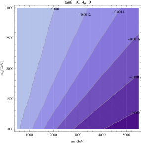
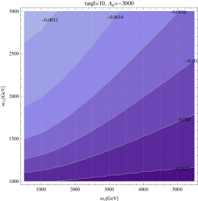
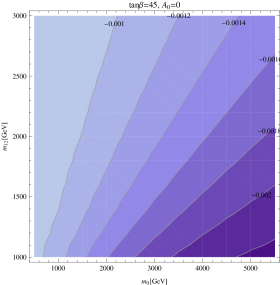
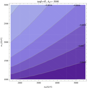
Figure 1: Contours of $\delta^{QLL}_{13}$ in the $m_{0}$–$m_{1/2}$ plane for different values of $\tan\beta$ and $A_{0}$ in the CMSSM.

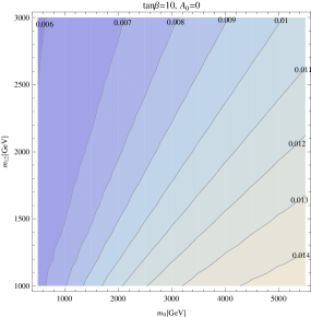
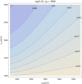
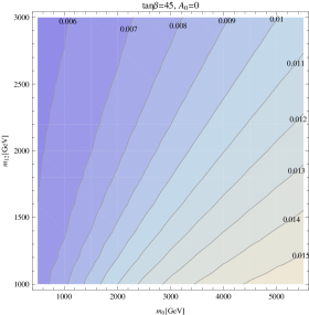
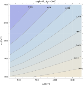
Figure 2: Contours of $\delta^{QLL}_{23}$ in the $m_{0}$–$m_{1/2}$ plane for different values of $\tan\beta$ and $A_{0}$ in the CMSSM.

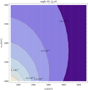
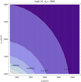
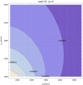
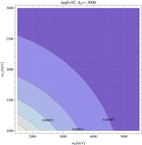
Figure 3: Contours of $\delta^{ULR}_{23}$ in the $m_{0}$–$m_{1/2}$ plane for different values of $\tan\beta$ and $A_{0}$ in the CMSSM.

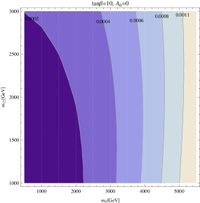
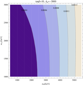
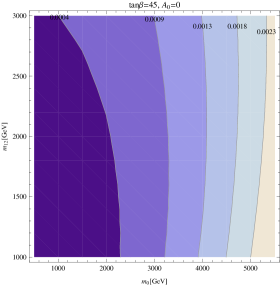
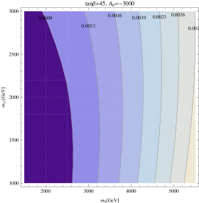
Figure 4: Contours of $\Delta\rho^{\rm MFV}$ in the $m_{0}$–$m_{1/2}$ plane for different values of $\tan\beta$ and $A_{0}$ in the CMSSM.

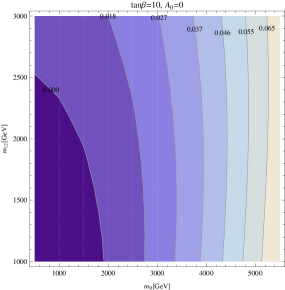
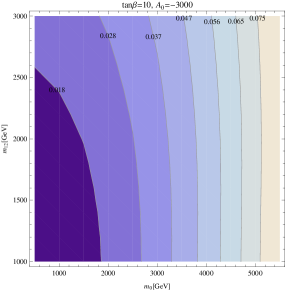
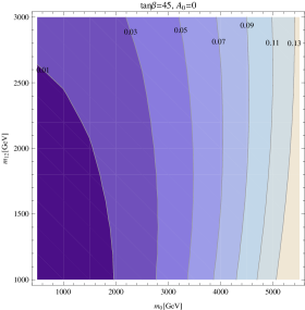
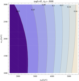
Figure 5: Contours of $\Delta M_{W}^{\rm MFV}$ in GeV in the $m_{0}$–$m_{1/2}$ plane for different values of $\tan\beta$ and $A_{0}$ in the CMSSM.

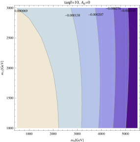
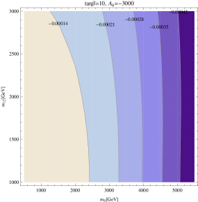
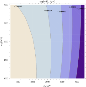
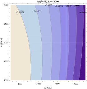
Figure 6: Contours of $\Delta\sin^{2}\theta_{\mathrm{eff}}^{\rm MFV}$ in the $m_{0}$–$m_{1/2}$ plane for different values of $\tan\beta$ and $A_{0}$ in the CMSSM.

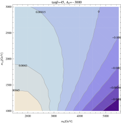
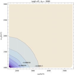
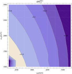
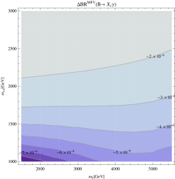
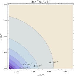
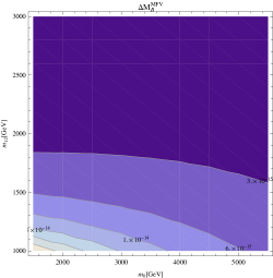
Figure 7: Contours of Higgs mass corrections ($\Delta M_{h}^{\rm MFV}$, $\Delta M_{H}^{\rm MFV}$ and $\Delta M_{H^{\pm}}^{\rm MFV}$ in GeV) and BPO ($\Delta{\rm BR}^{\rm MFV}(B\to X_{s}\gamma)$, $\Delta{\rm BR}^{\rm MFV}(B_{s}\to\mu^{+}\mu^{-})$ and $\Delta M_{B_{s}}^{\rm MFV}$) in the $m_{0}$–$m_{1/2}$ plane for $\tan\beta=45$ and  $A_{0}=-3000\,\,\mathrm{GeV}$ in the CMSSM.

4.2 Effects of slepton mixing.

In this section we analyze the effects of non-zero $\delta^{FAB}_{ij}$ values in the CMSSM-seesaw I. In order to investigate the effects induced just by the mixings in the slepton sector, such that we can compare their contribution from the one produced by the mixings in the squak sector (and to discriminate it from effects from mixings in the squark sector) we present here the results with only $\delta^{FAB}_{ij}$ in the slepton sector non-zero, i.e. after the RGE running with both CKM and see-saw parameters non-zero, the $\delta^{FAB}_{ij}$ from the squark sector are set to zero by hand at the EW scale. The effects of the squark mixing in the CMSSM-seesaw I are nearly indistinguishable from the ones analyzed in the previous subsection.

As mentioned in Sect. 2.2, the calculations in this section are done by using the values of $Y_{\nu}$ constructed from Eq. (11) with degenerate $M_{R}$’s. The matrix $R$ is set to the identity since it does not enter in Eq. (13) and therefore the slepton $\delta^{FAB}_{ij}$’s do not depend on it. The matrix $m_{\nu}^{\delta}$ is a diagonal mass matrix adjusted to reproduce neutrino masses at low energy compatible with the experimental observations and with hierarchical neutrino masses. We performed our computation by using the seesaw scale $M_{N}=10^{14}\,\,\mathrm{GeV}$. With this choice the bound $BR(\mu\to e\gamma)<5.7\times 10^{-13}$  [58] imposes severe restrictions on the $m_{0}$–$m_{1/2}$ plane, excluding values of $m_{0}$ below 2–3 TeV (depending on $\tan\beta$ and $A_{0}$). The values of the slepton $\delta^{FAB}_{ij}$ will increase as the scale $M_{N}$ increases but also does the parameter space excluded by the ${\rm BR}(\mu\to e\gamma)$ bound. For example, by increasing $M_{N}$ by an order of magnitude, the largest entries in the matrix $Y_{\nu}$ will become of ${\cal O}(1)$ and the bound on ${\rm BR}(\mu\to e\gamma)$ will only be satisfied if $m_{0}\approx 5\,\,\mathrm{TeV}$.

Our numerical results in the CMSSM-seesaw I are shown in Figs. 8 - 14. As in the CMSSM we present the results in the $m_{0}$–$m_{1/2}$ plane for four combinations of $\tan\beta=10,45$ (upper and lower row) and $A_{0}=0,-3000\,\,\mathrm{GeV}$ (left and right column), again capturing the “extreme” cases. We start presenting the three most relevant $\delta^{FAB}_{ij}$. Figs. 8-10 show $\delta^{LLL}_{12}$, $\delta^{LLL}_{13}$ and $\delta^{LLL}_{23}$, respectively. As expected, $\delta^{LLL}_{23}$ turns out to be largest of ${\cal O}(0.01)$, while the other two are about one order of magnitude smaller. The dependence on $\tan\beta$ is not very prominent, but going from $A_{0}=0$ to $-3000\,\,\mathrm{GeV}$ has a strong impact on the $\delta^{FAB}_{ij}$. For small $A_{0}$ the size of the $\delta^{FAB}_{ij}$ is increasing with larger $m_{0}$ and $m_{1/2}$, for $A_{0}=-3000\,\,\mathrm{GeV}$ the largest values are found for small $m_{0}$ and $m_{1/2}$. Here one comment on flavor violating decays is in order. The selected values of $Y_{\nu}$ result in a large prediction for, e.g., BR($\mu\to e\gamma$) that can eliminate some of the $m_{0}$–$m_{1/2}$ parameter plane, in particular combinations of low values of $m_{0}$ and $m_{1/2}$. For our parameter settings these regions are small for $\tan\beta=10$ and reach up to roughly $m_{0}+m_{1/2}\sim 2000\,\,\mathrm{GeV}$ for $A_{0}=-3000\,\,\mathrm{GeV}$. For $\tan\beta=45$ they are larger and exclude roughly the lower left half of the $m_{0}$–$m_{1/2}$ planes shown.

In Figs. 11-13 we show the results for the EWPO. The same pattern and non-decoupling behavior for EWPO as in the case of CMSSM (squark $\delta^{FAB}_{ij}$) can be observed. However, the corrections induced by slepton flavor violation are relatively small compared to squark case. For the most extreme cases, i.e. the largest values of $m_{0}$, the corrections to $M_{W}$ turn out to be of the same order of the experimental uncertainty. For those parts of the parameter space neglecting the effects of LFV to the EWPO could turn out to be an insufficient approximation, in particular in view of future improved experimental accuracies.

Finally, in Fig. 14 we present the corrections to the Higgs boson masses induced by slepton flavor violation. Here we only show $\Delta M_{h}^{\rm MFV}$ (left) and $\Delta M_{H^{\pm}}^{\rm MFV}$(right) for $\tan\beta=10$ and $A_{0}=0$. They turn out to be negligibly small in both cases. Corrections to $\Delta M_{H}^{\rm MFV}$, which are not shown, are even smaller. We have checked that these results hold also for other combinations of $\tan\beta$ and $A_{0}$. Consequently, within the Higgs sector the approximation of neglecting the effects of the $\delta^{FAB}_{ij}$ is fully justified.

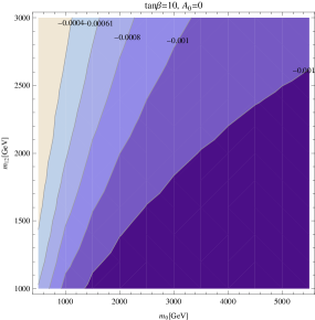
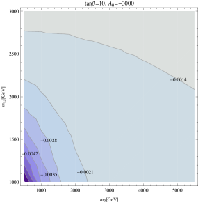
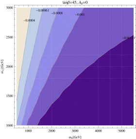
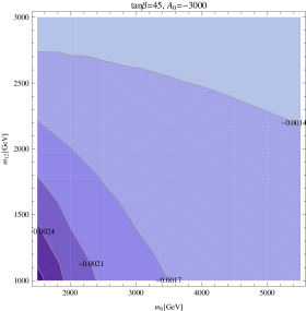
Figure 8: Contours of $\delta^{LLL}_{12}$ in the $m_{0}$–$m_{1/2}$ plane for different values of $\tan\beta$ and $A_{0}$ in the CMSSM-seesaw I.

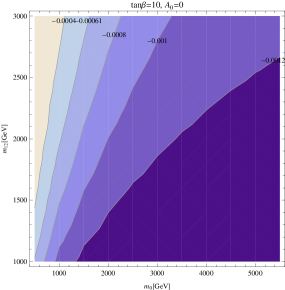
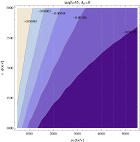
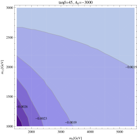
Figure 9: Contours of $\delta^{LLL}_{13}$ in the $m_{0}$–$m_{1/2}$ plane for different values of $\tan\beta$ and $A_{0}$ in the CMSSM-seesaw I.

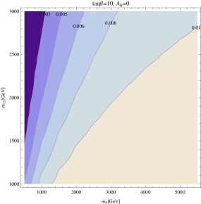
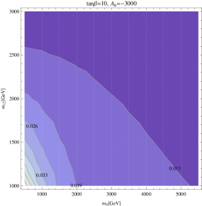
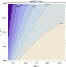
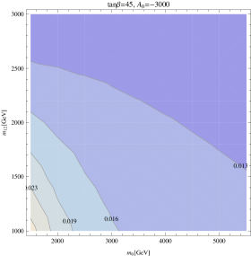
Figure 10: Contours of $\delta^{LLL}_{23}$ in the $m_{0}$–$m_{1/2}$ plane for different values of $\tan\beta$ and $A_{0}$ in the CMSSM-seesaw I.

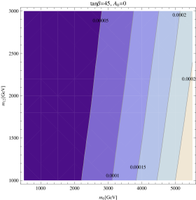
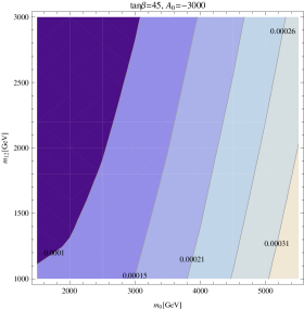
Figure 11: Contours of $\Delta\rho^{\rm MFV}$ in the $m_{0}$–$m_{1/2}$ plane for different values of $\tan\beta$ and $A_{0}$ in the CMSSM-seesaw I.

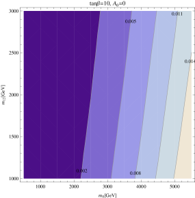
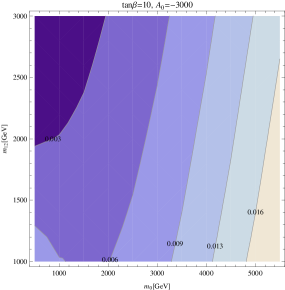
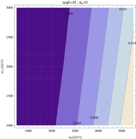
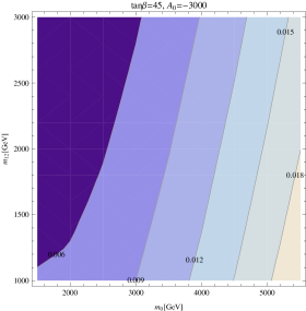
Figure 12: Contours of $\Delta M_{W}^{\rm MFV}$ in GeV in the $m_{0}$–$m_{1/2}$ plane for different values of $\tan\beta$ and $A_{0}$ in the CMSSM-seesaw I.

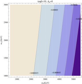
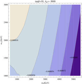
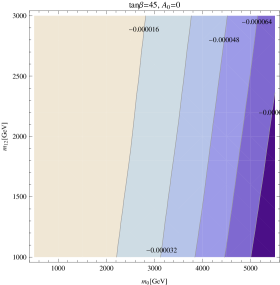
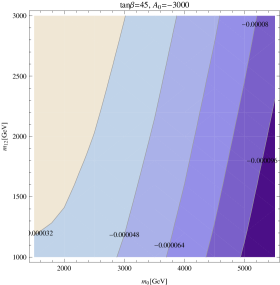
Figure 13: Contours of $\Delta\sin^{2}\theta_{\mathrm{eff}}^{\rm MFV}$ in the $m_{0}$–$m_{1/2}$ plane for different values of $\tan\beta$ and $A_{0}$ in the CMSSM-seesaw I.

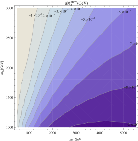
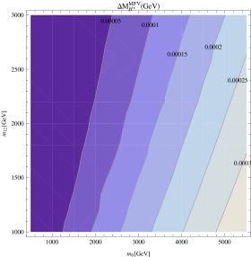
Figure 14: Contours of $\Delta M_{h}^{\rm MFV}$ (left) and $\Delta M_{H^{\pm}}^{\rm MFV}$ (right) in the $m_{0}$–$m_{1/2}$ plane for $\tan\beta=10$ and $A_{0}=0$ in the CMSSM-seesaw I.

5 Conclusions

In this paper we have investigated the CMSSM and the CMSSM-seesaw I (i.e. the CMSSM augmented by right-handed neutrinos to produce the observed neutrino mass pattern via the seesaw type I mechanism) under the hypothesis of Minimal Flavor Violation (MFV, i.e. the only flavor violating source is the CKM matrix and/or the PMNS matrix in the case of the CMSSM-seesaw I). In many phenomenological analyses of the CMSSM the effects of intergenerational mixing in the squark and/or slepton sector is neglected. However, such mixings are naturally induced, assuming no flavor violation at the GUT scale, by the RGE running from the GUT to the EW scale exactly due to the presence of the CKM and/or the PMNS matrix. The spectra of the CMSSM and CMSSM-seesaw I have been evaluated with the help of the program SPheno by taking the GUT scale input run down via the appropriate RGEs to the EW scale.

We have evaluated the predictions for $B$-physics observables, MSSM Higgs boson masses, electroweak precision observables in the CMSSM and CMSSM-seesaw I. In order to analyze the effects of neglecting intergenerational mixing these observables have been evaluated with the full spectrum at the EW scale, as well as with the spectrum, but with all intergenerational mixing set (artificially) to zero (as it has been done in many phenomenological analyses). The difference in the various observables indicates the size of the effects neglected in those analyses. In this way it can be checked whether neglecting those mixing effects is a justified approximation.

Within the CMSSM we have taken a fixed grid of $A_{0}$ and $\tan\beta$, while scanning the $m_{0}$–$m_{1/2}$ plane. We found that the value of $\delta^{FAB}_{ij}$ increases with the increase of the $A_{0}$ or $\tan\beta$ values. The Higgs boson masses receive corrections below current and future experimental uncertainties, where the shifts in $M_{H^{\pm}}$ were found largest at the level of ${\cal O}(100\,\,\mathrm{MeV})$. Similarly for the $B$-physics observables the induced effects are at least one order of magnitude smaller than the current experimental uncertainty. For those two groups of observables the approximation of neglecting intergenerational mixing explicitly is a viable option.

The picture changes for the electroweak precision observables. The masses of the squarks grow with $m_{0}$, and thus do the mixing terms, inducing a splitting between masses in an $SU(2)$ doublet, leading to a non-decoupling effect. For $m_{0}\;\raisebox{-3.00003pt}{$\stackrel{{\scriptstyle\displaystyle>}}{{\sim}}$}\;3\,\,\mathrm{TeV}$ the effects induced in $M_{W}$ and $\sin^{2}\theta_{\mathrm{eff}}$ are several times larger than the current experimental uncertainties and can shift the CMSSM prediction outside the allowed experimental range. In this way, taking the intergenerational mixing (correctly) into account can set an upper bound on $m_{0}$ that is not present in recent phenomenological analyses.

Going to the CMSSM-seesaw I the numerical results depend on the concrete model definition. We have chosen a set of parameter that reproduces correctly the observed neutrino data and simultaneously induces large LFV effects and induces relatively large corrections to the calculated observables. Consequently, parts of the parameter space are excluded by the experimental bounds on ${\rm BR}(\mu\to e\gamma)$. Concerning the precision observables we find that $B$-physics observables are not affected, we also find that the additional effects induced by slepton flavor violation on Higgs boson masses are negligible. Again the EWPO show the largest impact, where for $M_{W}$ effects at the same level as the current experimental accuracy can be observed for very large values of $m_{0}$.

To summarize: artificially setting all flavor violating terms to zero in the CMSSM and CMSSM-seesaw I is an acceptable approximation for $B$-physics observables, Higgs boson masses. However, in the electroweak precision observables the flavor violation in the MFV framework induced by the presence of the CKM matrix in the RGE running from the GUT to the EW scale large effects can be induced. Those effects can be substantially larger than the current experimental accuracy in $M_{W}$ and $\sin^{2}\theta_{\mathrm{eff}}$. Taking those effects correctly into account places new upper bounds on $m_{0}$ that are neglected in recent phenomenological analyses.

Acknowledgments

The work of S.H. and M.R. was partially supported by CICYT (grant FPA 2013-40715-P). M.G., S.H. and M.R. were supported by the Spanish MICINN’s Consolider-Ingenio 2010 Programme under grant MultiDark CSD2009-00064. M.E.G.  acknowledges further support from the MICINN project FPA2011-23781

References

-
[1]
H. Nilles,
Phys. Rept. 110 (1984) 1;
H. Haber and G. Kane, Phys. Rept. 117 (1985) 75;
R. Barbieri, Riv. Nuovo Cim. 11 (1988) 1. - [2] Y. Amhis et al. [Heavy Flavor Averaging Group], arXiv:1207.1158 [hep-ex] SLAC-R-1002, FERMILAB-PUB-12-871-PPD
-
[3]
R. Chivukula and H. Georgi,
Phys. Lett. B 188 (1987) 99;
L. Hall and L. Randall, Phys. Rev. Lett. 65 (1990) 2939;
A. Buras et al., Phys. Lett. B 500 (2001) 161. - [4] G. D’Ambrosio et al., Nucl. Phys. B 645 (2002) 155.
- [5] S. S. AbdusSalam et al., Eur. Phys. J. C 71 (2011) 1835 [arXiv:1109.3859 [hep-ph]].
- [6] F. Borzumati and A. Masiero, Phys. Rev. Lett. 57 (1986) 961.
-
[7]
S. Fukuda et al. [Super-Kamiokande Collaboration],
Phys. Rev. Lett. 86 (2001) 5656
[arXiv:hep-ex/0103033];
S. Fukuda et al. [Super-Kamiokande Collaboration], Phys. Rev. Lett. 86 (2001) 5651 [arXiv:hep-ex/0103032];
S. Fukuda et al. [Super-Kamiokande Collaboration], Phys. Lett. B 539 (2002) 179 [arXiv:hep-ex/0205075];
M. Apollonio et al. [CHOOZ Collaboration], Phys. Lett. B 466 (1999) 415 [arXiv:hep-ex/9907037];
Q. Ahmad et al. [SNO Collaboration], Phys. Rev. Lett. 87 (2001) 071301 [arXiv:nucl-ex/0106015];
Q. Ahmad et al. [SNO Collaboration], Phys. Rev. Lett. 89 (2002) 011301 [arXiv:nucl-ex/0204008];
M. Ambrosio et al. [MACRO Collaboration], Phys. Lett. B 517 (2001) 59;
G. Giacomelli and M. Giorgini [MACRO Collaboration], arXiv:hep-ex/0110021;
K. Eguchi et al. [KamLAND Collaboration], arXiv:hep-ex/0212021. - [8] V. Cirigliano et al. Nucl. Phys. B 728 (2005) 121 [arXiv:hep-ph/0507001].
-
[9]
P. Minkowski,
Phys. Lett. B 67 (1977) 421;
M. Gell-Mann, P. Ramond and R. Slansky, in Complex Spinors and Unified Theories eds. P. Van. Nieuwenhuizen and D. Freedman, Supergravity (North-Holland, Amsterdam, 1979), p.315 [Print-80-0576 (CERN)];
T. Yanagida, in Proceedings of the Workshop on the Unified Theory and the Baryon Number in the Universe, eds. O. Sawada and A. Sugamoto (KEK, Tsukuba, 1979), p.95;
S. Glashow, in Quarks and Leptons, eds. M. Lévy et al. (Plenum Press, New York, 1980), p.687;
R. Mohapatra and G. Senjanović, Phys. Rev. Lett. 44 (1980) 912. -
[10]
O. Buchmueller et al.,
Eur. Phys. J. C 74 (2014) 12, 3212
[arXiv:1408.4060 [hep-ph]];
O. Buchmueller et al., Eur. Phys. J. C 74 (2014) 2922 [arXiv:1312.5250 [hep-ph]];
O. Buchmueller et al., Eur. Phys. J. C 72 (2012) 2243 [arXiv:1207.7315 [hep-ph]];
O. Buchmueller et al., Eur. Phys. J. C 72 (2012) 1878 [arXiv:1110.3568 [hep-ph]]. - [11] W. Porod, Comput. Phys. Commun. 153 (2003) 275 [arXiv:hep-ph/0301101].
-
[12]
P. Skands et al.,
JHEP 0407 (2004) 036
[arXiv:hep-ph/0311123];
B. Allanach et al., Comput. Phys. Commun. 180 (2009) 8 [arXiv:0801.0045 [hep-ph]]. -
[13]
S. Heinemeyer, W. Hollik and G. Weiglein,
Comput. Phys. Commun. 124 (2000) 76
[arXiv:hep-ph/9812320];
T. Hahn, S. Heinemeyer, W. Hollik, H. Rzehak and G. Weiglein, Comput. Phys. Commun. 180 (2009) 1426; see www.feynhiggs.de . - [14] S. Heinemeyer, W. Hollik and G. Weiglein, Eur. Phys. J. C 9 (1999) 343 [arXiv:hep-ph/9812472].
- [15] G. Degrassi, S. Heinemeyer, W. Hollik, P. Slavich and G. Weiglein, Eur. Phys. J. C 28 (2003) 133 [arXiv:hep-ph/0212020].
- [16] M. Frank, T. Hahn, S. Heinemeyer, W. Hollik, R. Rzehak and G. Weiglein, JHEP 0702 (2007) 047 [arXiv:hep-ph/0611326].
- [17] T. Hahn, S. Heinemeyer, W. Hollik, H. Rzehak and G. Weiglein, Phys. Rev. Lett. 112 (2014) 141801 [arXiv:1312.4937 [hep-ph]].
-
[18]
G. Isidori and P. Paradisi,
Phys. Lett. B 639 (2006) 499
[arXiv:hep-ph/0605012];
G. Isidori, F. Mescia, P. Paradisi and D. Temes, Phys. Rev. D 75 (2007) 115019 [arXiv:hep-ph/0703035], and references therein. - [19] M. Arana-Catania, S. Heinemeyer, M. Herrero and S. Peñaranda, JHEP 1205 (2012) 015 [arXiv:1109.6232 [hep-ph]]; arXiv:1201.6345 [hep-ph].
- [20] M. Arana-Catania, S. Heinemeyer and M. J. Herrero, Phys. Rev. D 90 (2014) 075003 [arXiv:1405.6960 [hep-ph]].
- [21] N. Falck, Z. Phys. C 30 (1986) 247.
- [22] S. Bertolini, F. Borzumati, A. Masiero, and G. Ridolfi, Nucl. Phys. B 353 (1991) 591.
- [23] J. Hisano, T. Moroi, K. Tobe and M. Yamaguchi, Phys. Rev. D 53 (1996) 2442.
- [24] M. Cannoni, J. Ellis, M. Gómez and S. Lola, Phys. Rev. D 88 (2013) 7, 075005 [arXiv:1301.6002 [hep-ph]].
- [25] M. Gómez, G. Leontaris, S. Lola and J. Vergados, Phys. Rev. D 59 (1999) 116009 [arXiv:hep-ph/9810291].
- [26] J. Ellis, M. E. Gómez, G. Leontaris, S. Lola and D. Nanopoulos, Eur. Phys. J. C 14 (2000) 319 [arXiv:hep-ph/9911459].
- [27] S. Antusch, E. Arganda, M. Herrero and A. Teixeira, JHEP 0611 (2006) 090 [arXiv:hep-ph/0607263].
- [28] J. Ellis, M. Gómez and S. Lola, JHEP 0707 (2007) 052 [arXiv:hep-ph/0612292].
- [29] J. Casas and A. Ibarra, Nucl. Phys. B 618 (2001) 171 [arXiv:hep-ph/0103065].
- [30] G. Fogli, E. Lisi, A. Marrone, D. Montanino, A. Palazzo and A. Rotunno, Phys. Rev. D 86 (2012) 013012 [arXiv:1205.5254 [hep-ph]].
- [31] M. Gómez, T. Hahn, S. Heinemeyer, M. Rehman, Phys. Rev. D 90 (2014) 074016 [arXiv:1408.0663 [hep-ph]].
- [32] M. Arana-Catania, S. Heinemeyer and M. Herrero, Phys. Rev. D 88 1 (2013) 015026 [arXiv:1304.2783 [hep-ph]].
- [33] Y. Kuno and Y. Okada, Rev. Mod. Phys. 73 (2001) 151 [arXiv:hep-ph/9909265].
-
[34]
S. Bilenky, S. Petcov and B. Pontecorvo,
Phys. Lett. B 67 (1977) 309;
W. Marciano and A. Sanda, Phys. Lett. B 67 (1977) 303. - [35] T. Cheng, L.-F. Li, Phys. Rev. Lett. 45 (1980) 1908.
-
[36]
A. Djouadi,
Phys. Rept. 459 (2008) 1
[arXiv:hep-ph/0503173];
S. Heinemeyer, Int. J. Mod. Phys. A 21 (2006) 2659 [arXiv:hep-ph/0407244]. - [37] G. Aad et al. [ATLAS Collaboration], Phys. Rev. D 90 (2014) 052004 [arXiv:1406.3827 [hep-ex]].
- [38] CMS Collaboration [CMS Collaboration], CMS-PAS-HIG-14-009.
- [39] H. Baer et al., arXiv:1306.6352 [hep-ph].
- [40] S. Gennai et al. Eur. Phys. J. C 52 (2007) 383 [arXiv:0704.0619 [hep-ph]].
- [41] S. Heinemeyer, W. Hollik, F. Merz, S. Peñaranda, Eur. Phys. J. C 37 (2004) 481 [arXiv:hep-ph/0403228].
- [42] S. Heinemeyer, W. Hollik and G. Weiglein, Phys. Rept. 425 (2006) 265 [arXiv:hep-ph/0412214].
-
[43]
S. Schael et al. [ALEPH and DELPHI and L3 and OPAL and LEP
Electroweak Collaborations],
Phys. Rept. 532 (2013) 119
[arXiv:1302.3415 [hep-ex]];
see http://www.cern.ch/LEPEWWG . -
[44]
M. Baak et al., arXiv:1310.6708 [hep-ph];
A. Freitas et al., arXiv:1307.3962 [hep-ph]. -
[45]
S. Heinemeyer,
talk given at the 8th FCC-ee Physics Workshop,
Paris, France, October 2014, see:
https://indico.cern.ch/event/337673/session/3/contribution/
41/material/slides . - [46] M. Veltman, Nucl. Phys. B 123 (1977) 89.
- [47] G. Isidori and A. Retico, JHEP 0209 (2002) 063 [arXiv:hep-ph/0208159].
- [48] P. Chankowski and L. Slawianowska, Phys. Rev. D 63 (2001) 054012 [arXiv:hep-ph/0008046].
- [49] J. Foster, K. Okumura and L. Roszkowski, JHEP 0508 (2005) 094 [arXiv:hep-ph/0506146].
-
[50]
See: https://www.slac.stanford.edu/xorg/hfag/rare/2013/radll/
OUTPUT/TABLES/radll.pdf . - [51] M. Misiak, Acta Phys. Polon. B 40 (2009) 2987 [arXiv:0911.1651 [hep-ph]].
- [52] S. Chatrchyan et al. [CMS Collaboration], Phys. Rev. Lett. 111 (2013) 101804 [arXiv:1307.5025 [hep-ex]].
- [53] R. Aaij et al. [LHCb Collaboration], Phys. Rev. Lett. 111 (2013) 101805 [arXiv:1307.5024 [hep-ex]].
- [54] A. Buras, J. Girrbach, D. Guadagnoli and G. Isidori, Eur. Phys. J. C 72 (2012) 2172 [arXiv:1208.0934 [hep-ph]].
- [55] See: https://www.slac.stanford.edu/xorg/hfag/osc/PDG_2013/ .
- [56] A. Buras, M. Jamin and P. Weisz, Nucl. Phys. B 347 (1990) 491.
- [57] E. Golowich, J. Hewett, S. Pakvasa, A. Petrov and G. Yeghiyan, Phys. Rev. D 83 (2011) 114017 [arXiv:1102.0009 [hep-ph]].
- [58] J. Adam et al. [MEG Collaboration], arXiv:1303.0754 [hep-ex].